
Abstract
Analytical theory for second harmonic nonlinear electrochemical impedance spectroscopy (2nd-NLEIS) of planar and porous electrodes is developed for interfaces governed by Butler-Volmer kinetics, a Helmholtz (mainly) or Gouy-Chapman (introduced) double layer, and transport by ion migration and diffusion. A continuum of analytical EIS and 2nd-NLEIS models is presented, from nonlinear Randles circuits with or without diffusion impedances to nonlinear macrohomogeneous porous electrode theory that is shown to be analogous to a nonlinear transmission-line model. EIS and 2nd-NLEIS for planar electrodes share classic charge transfer RC and diffusion time-scales, whereas porous electrode EIS and 2nd-NLEIS share three characteristic time constants. In both cases, the magnitude of 2nd-NLEIS is proportional to nonlinear charge transfer asymmetry and thermodynamic curvature parameters. The phase behavior of 2nd-NLEIS is more complex and model-sensitive than in EIS, with half-cell NLEIS spectra potentially traversing all four quadrants of a Nyquist plot. We explore the power of simultaneously analyzing the linear EIS and 2nd-NLEIS spectra for two-electrode configurations, where the full-cell linear EIS signal arises from the sum of the half-cell spectra, while the 2nd-NLEIS signal arises from their difference.

Export citation and abstract BibTeX RIS

This is an open access article distributed under the terms of the Creative Commons Attribution 4.0 License (CC BY, http://creativecommons.org/licenses/by/4.0/), which permits unrestricted reuse of the work in any medium, provided the original work is properly cited.
List of Variables

| Faradaic current density 
|

| Non-faradaic current density 
|

| Exchange current density 
|

| Anodic charge transfer coefficient |

| Cathodic charge transfer coefficient |

| Charge transfer symmetry parameter |

| Number of electrons involved per electrochemical reaction |

| Faraday constant ( ) ) |

| Gas constant ( ) ) |

| Temperature ( ) ) |


| Measured overpotential ( ) ) |

| Solid phase potential ( ) ) |

| Ionic conducting phase potential ( ) ) |


| Equilibrium polarization ( ) ) |

| Reciprocal of thermal voltage 
|

| Double layer capacitance per unit area 
|

| Interfacial area ( ) ) |

| Thickness of the electrode ( ) ) |

| Area of the pores per unit volume on which the double layer can be formed ( ) ) |

| Resistivity of pore electrolyte ( ) ) |

| Imposed current ( ) ) |

| Amplitude of the imposed current ( ) ) |

| Frequency of imposed current ( ) ) |

| Complex magnitude of measured overpotential at  ( ( ) ) |

| Complex magnitude of measured overpotential at 2  ( ( ) ) |

| First harmonic impedance coefficient ( ) ) |

| Second harmonic impedance coefficient 
|

| Charge transfer resistance of the interface or porous electrode ( ) ) |

| Double layer capacitance of the interface or porous electrode ( ) ) |

| Dimensionless frequency related to charge transfer resistance |

| Effective pore electrolyte resistance across the entire porous electrode ( ) ) |

| Dimensionless frequency related to pore electrolyte resistance |

| Ion concentration in the solid phase 
|

| Faradaic current ( ) ) |

| Bounded diffusion impedance ( ) ) |

| Thermodynamic parameter 
|

| Diffusion time constant ( ) ) |

| Characteristics length scale for diffusion ( ) ) |

| Diffusion coefficient of the electroactive species 
|

| Bounded diffusion impedance coefficient ( ) ) |

| Interfacial area of the electrode ( ) ) |

| Electron charge ( ) ) |
Electrochemical impedance spectroscopy (EIS) is a widely used electroanalytical technique for studying fundamental and applied aspects of corrosion, 1,2 biosensors, 3,4 fuel cells, 5,6 and batteries. 7,8 EIS probes the linear frequency response of electrochemical interfaces. Yet, electrochemical interfaces are inherently nonlinear, so the mathematics that underpins EIS analysis is an approximation that holds in the limit of infinitesimal current or voltage modulations, where nonlinearity-generated higher-order responses can be ignored. In practice, a rule of thumb for experiments is that interfacial modulations under 5 mV are sufficiently small for linear analysis, though tests are available to ensure real data meets linearity and stationarity assumptions. 9,10 Linearization of a nonlinear system results in a loss of information and introduces the potential for degeneracy in both equivalent circuit-based and physics-based analysis, sometimes limiting the mechanistic discriminating power of EIS. 11,12 Two distinct approaches have emerged to explore the frequency response of electrochemical interfaces beyond the infinitesimal linear response limit, namely, probing the weakly nonlinear response with modulations just larger than the linear limits 13 or strongly nonlinear responses from large modulations that drive complex nonlinear system dynamics. 14 Here we focus on weak nonlinearity as it has the discriminating power of nonlinear analysis while maintaining moderate amplitude modulations that are less likely to damage the electrochemical interface(s) under test.
Perhaps the most studied weakly nonlinear electroanalytical technique is faradaic rectification, a method that relies on moderate amplitude current modulations of the electrochemical interface to generate measurable frequency-dependent shifts of the mean voltage under conditions of zero mean current. 15,16 As with linear EIS, practitioners of faradaic rectification have identified tests for whether current modulations are sufficient to excite 2nd-order nonlinear processes without over driving the system (thereby complicating analysis); a rule of thumb is that current modulations should produce under 20 mV of voltage oscillation. 17 Other examples of weakly nonlinear frequency response methods in electrochemistry include more specialized techniques such as nonlinear hydrodynamic modulation voltammetry (HMV). 18,19 In HMV, experiments and theory can measure and explain frequency-dependent limiting current behaviors that result from second-order Reynolds stress rectification of flow, creating an HMV-analog of faradaic rectification, 20 as well as probe and understand complex magnitude and phase behaviors of oscillating limiting current harmonics that occur in second- and higher-order nonlinear processes. 21 Faradaic rectification and nonlinear HMV are mainly applied to fairly simple electroanalytical half-cell configurations with planar interfaces, where transport is neglected or carefully controlled via a rotating disc electrode.
Probing the weakly nonlinear response of more complex porous electrode configurations, such as those used in electrochemical energy applications, is a rather new extension of linear EIS. Wilson et al. looked at third harmonic nonlinear electrochemical impedance spectroscopy (3rd-NLEIS) to qualitatively discriminate among multiple oxygen reduction mechanisms in symmetric cells with two identical porous solid oxide fuel cell (SOFC) electrodes. 12 Murbach et al. showed the power of second harmonic NLEIS (2nd-NLEIS) when using two dissimilar electrodes in a battery configuration, which produced full-cell responses with both even and odd harmonic NLEIS spectra. 22 Physics-based analysis showed that 2nd-NLEIS provides access to interfacial processes not measurable with linearized EIS and, importantly, the presence of a 2nd-NLEIS signal need not alter the analysis of traditional EIS, as long as the driving current modulation amplitude is small enough to avoid third-order nonlinear processes. 23 In practice, this means selecting a current modulation that produces a measurable second harmonic in the output voltage spectrum without also generating measurable third- or higher-harmonics. 22 While the most direct way to assess the appropriate current modulation amplitudes for 2nd-NLEIS is through analysis of the voltage spectrum, a rule of thumb is that input current modulations should produce voltage modulations above 5 mV (the typical linear limit) and below 20 mV (the typical faradaic rectification limit) to avoid over-driving nonlinear processes and corrupting the linear response. 22
As Wilson, et al. 12 and Murbach et al. 22,23 have shown, physics-based NLEIS modeling and complementary experiments provide powerful mechanistic discrimination and insights for porous electrodes in complex electrochemical configurations, but these complex models have not been useful for parameter estimation from datasets. Recently, a nonlinear single particle model (SPM) has been developed by Kirk et al. to quantitively analyze 2nd-NLEIS spectra for commercial Li-ion batteries; this represents, to the best of our knowledge, the first model-based analysis of 2nd-NLEIS data. 24 The battery datasets fit by Kirk et al. showed the classical EIS depressed interfacial charge transfer behavior that is attributable to co-limiting ohmic and charge transfer within the porous battery electrodes; 24 co-limiting physics is not captured by SPM models where no ohmic variation or current density variation is allowed to occur in the porous electrode. In short, the P2D-based models in Murbach et al. were too complex for quantitative analysis of battery EIS and 2nd-NLEIS data, whereas Kirk et al. demonstrated the power of parameter estimation with simple models, but the specific model used excluded essential physics seen in the battery dataset.
In this work, we seek to develop a continuum of increasingly sophisticated modeled physics—from nonlinear Randles circuits and nonlinear SPMs to simplified nonlinear porous electrodes—in order to explore the essential drivers of 2nd-NLEIS, and the ways linear EIS and 2nd-NLEIS complement one another. We also explore the implications of a subtle point made by Murbach et al., 22 namely, the "parity rules" for NLEIS response when two half-cells are combined into a two-electrode cell. Specifically, the odd-harmonic NLEIS signals from half-cells add to produce the full-cell odd-harmonic NLEIS response, whereas even-harmonic NLEIS signals from two half-cells get subtracted to produce the full-cell even-harmonic NLEIS response. Here, we further elaborate on the impact of two-electrode cells having additive "positive parity" first harmonic (linear) EIS spectra and complementary subtractive "negative parity" 2nd-NLEIS spectra. One consequence of these harmonic "parity rules" can be seen in the symmetric two-electrode experiments reported by Wilson et al., 12 where only odd-harmonics were present in the NLEIS spectrum; in a symmetric cell, the identical 2nd-NLEIS half-cell signals nullify at all frequencies.
Overall, our goal here is to simplify the physics, analysis, and equivalent circuit representation of 2nd-NLEIS to chart a tractable and easy to implement quantitative analysis pathway that can be viewed as a natural extension of EIS for planar and porous electrode half-cells, as well as their combination into two-electrode configurations. This paper is accompanied by Part II, an experimental study to show model implementation.
Governing Physics for the Dynamics of Weakly Nonlinear Planar and Porous Electrodes
A key driver for the nonlinear response of an electrochemical interface is the charge transfer reaction. For a weakly nonlinear electrochemical interface, the faradaic current density ( ) is expressed using a two-term Taylor series expansion of the Butler–Volmer equation for small but finite overpotentials, i.e.,
  yielding


where  is the exchange current density (
 ),
),  is the interfacial potential difference (
 ) between the solid electrode and the ion-conducting electrolyte,
  is the equilibrium interfacial potential difference (
 ), and
  The parameter
  is a measure of charge transfer asymmetry (dimensionless) such that the anodic and cathodic charge transfer coefficients are
  and
and  respectively, with
  representing symmetric charge transfer. Finally, h.o.t. denotes the higher order terms of the Taylor series which we ignore here, but can be included in the description of the weakly nonlinear electrochemical interface as it is increasingly perturbed from equilibrium. Non-faradaic current (
 ) is treated with a simple (linear) constant-coefficient Helmholtz model:

where  is the double layer capacitance per unit interfacial area (
 ). Consequently, a planar electrochemical interface of area
  (
( ) has a total current (
 ) given by the sum of Eqs. 1 and 2 in the weakly nonlinear regime


Next, we formulate the weakly nonlinear governing equation for a porous electrode of thickness d ( ) on a current collector of area
  (
( ), where we denote the internal interfacial area per unit volume of the porous electrode as
  (
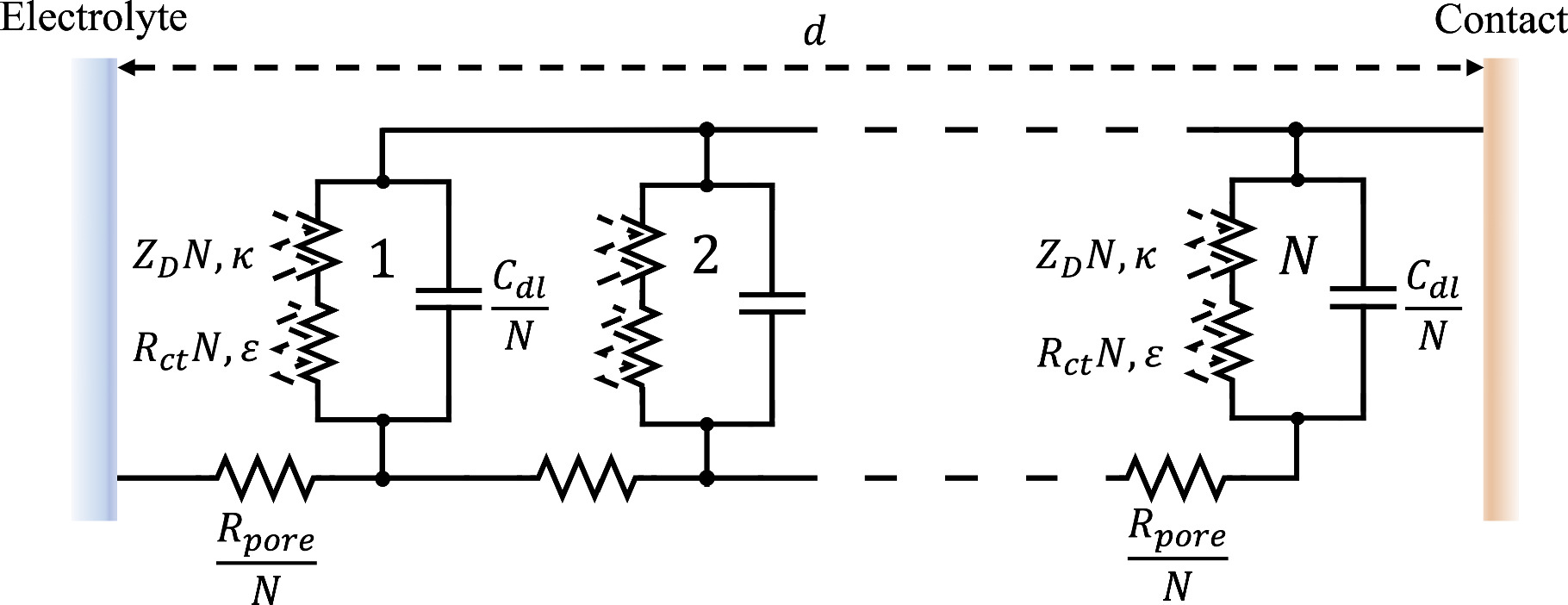
( ). Per the schematic in Fig. 1, bulk electrolyte contacting the electrolyte-filled porous electrode is located at
  and the current collector is at
  The weakly nonlinear behavior we explore here is a straightforward extension of the macrohomogeneous porous electrode theory developed by Paasch et al.,
25
except we use the two-term quadratic form of Eq. 1 instead of the single term linear response. Because most porous electrodes utilize a low resistivity solid relative to the ionic resistivity of the electrolyte in the pores, we simplify our formulation of Paasch's equations using a constant solid potential
The weakly nonlinear behavior we explore here is a straightforward extension of the macrohomogeneous porous electrode theory developed by Paasch et al.,
25
except we use the two-term quadratic form of Eq. 1 instead of the single term linear response. Because most porous electrodes utilize a low resistivity solid relative to the ionic resistivity of the electrolyte in the pores, we simplify our formulation of Paasch's equations using a constant solid potential  The resulting macrohomogeneous governing equation for charge conservation in the porous electrode domain, extended to the weakly nonlinear regime using Eq. 1, is


where  is the effective ionic resistivity of electrolyte (
 ) from volume-averaging the electrode pore-space.
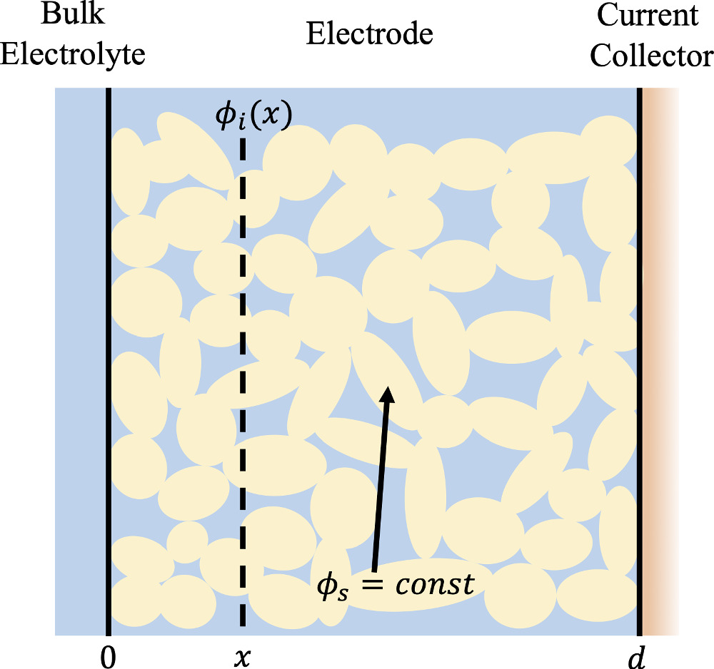
Figure 1. Two-dimensional schematic of a porous electrode with zero resistivity solid (yellow regions) and interconnected pores filled with an ion-conducting electrolyte phase (blue regions).
Download figure:
Standard image High-resolution imageCasting the governing equations into a weakly nonlinear impedance formalism
Electrochemical impedance spectroscopy (EIS) experiments impose a single frequency alternating current excitation to the electrode under study, represented here as

where 
 is the amplitude of the current modulation (Amp) with frequency
  (radians/s) For sufficiently small excitation amplitude
 , the voltage output for a stationary system is dominated by the linear response of the interface and produces a modulated voltage at the excitation frequency
  Murbach et al. has shown theoretically,
23
and validated experimentally,
22
that moderately larger amplitude single-frequency current excitations can generate a weakly nonlinear modulated voltage response of the form
Murbach et al. has shown theoretically,
23
and validated experimentally,
22
that moderately larger amplitude single-frequency current excitations can generate a weakly nonlinear modulated voltage response of the form

where the voltage output is at the excitation frequency  and the second harmonic
  To be consistent with Eq. 1, we ignore higher order terms generated at increasingly large current modulation amplitudes, but can direct the interested reader elsewhere for the formal solution structure for h.o.t.
12,26,27
As we have shown previously,
22
the linear and second harmonic impedances from the voltage spectrum represented by Eq. 6 are
To be consistent with Eq. 1, we ignore higher order terms generated at increasingly large current modulation amplitudes, but can direct the interested reader elsewhere for the formal solution structure for h.o.t.
12,26,27
As we have shown previously,
22
the linear and second harmonic impedances from the voltage spectrum represented by Eq. 6 are

and

where  is the complex frequency-dependent (linear) EIS and
  is the complex frequency-dependent second harmonic nonlinear EIS (2nd-NLEIS) function.
Mathematically, the EIS function  computed in Eq. 7 is identical to the comparable (linear) EIS spectrum when Eq. 6 represents the voltage spectrum; practically, we have shown that achieving Eq. 6 experimentally is straightforward.
22
In contrast, when the current amplitude is large enough to generate half-cell voltage spectra with three, four, or higher multiples of the excitation frequency, then
computed in Eq. 7 is identical to the comparable (linear) EIS spectrum when Eq. 6 represents the voltage spectrum; practically, we have shown that achieving Eq. 6 experimentally is straightforward.
22
In contrast, when the current amplitude is large enough to generate half-cell voltage spectra with three, four, or higher multiples of the excitation frequency, then  computed in Eq. 7 will have additional nonlinear contributions that deviate from the traditional (linear) response. Here, we only consider moderate modulation amplitudes consistent with Eq. 6.
Results and Discussion
The weakly nonlinear randles circuit
A planar electrochemical interface with time-invariant and uniform concentrations throughout the solid and electrolyte phases is governed by Eq. 3 with constant  For simplicity, we set
  and re-write Eq. 3 in terms of physically interpretable parameters common to a Randles circuit analysis, namely,

where  is the interfacial charge transfer resistance (
 ), and
  is the double layer capacitance of the interface (
 ). Since current generated through faradaic and non-faradaic processes are additive in Eq. 9, it represents parallel paths across the interface, akin to a Randles circuit but with an extra nonlinear charge transfer term that scales with the charge transfer symmetry parameter
To find  and
and  for this weakly nonlinear Randles circuit, we insert Eqs. 5 and 6 into Eq. 9, separate the equations into first harmonic (linear) terms multiplied by
  second harmonic terms multiplied by
  and ignore any higher harmonic terms. With algebraic manipulation, the governing equation for the complex interfacial voltage fluctuations at the excitation frequency
  is,
is,

and the second harmonic interfacial voltage at a frequency of  is
is

where  is the dimensionless frequency commonly used in Randles circuit analysis. Note that Eq. 11 shows that the second harmonic potential response (
 ) depends on the solution at the excitation frequency (
 ). Algebraic manipulation of Eq. 10, along with the use of Eq. 7, provides the classic linear Randles EIS frequency response at the first harmonic,

with real and imaginary parts given as

and

To find the weakly nonlinear 2nd-NLEIS response, Eq. 10 is rearranged and inserted into Eq. 11, then solved for  Using Eq. 8 provides the 2nd-NLEIS for the nonlinear Randles circuit,

which can be written as real and imaginary terms

and

Equation 13 shows the size of the 2nd-NLEIS response is directly proportional to the charge transfer asymmetry parameter (
 ), with the same characteristic
  time constant as is found in the linear EIS response.
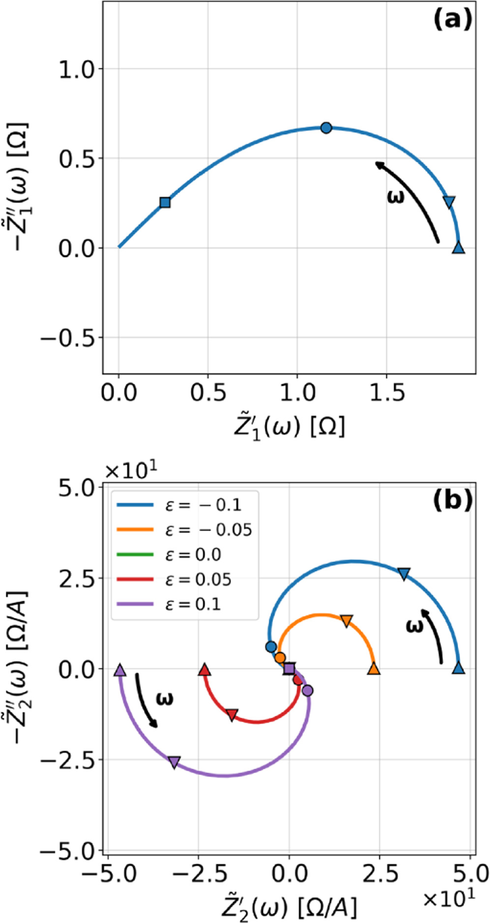
Figure 2 shows Nyquist plots for the first harmonic (linear) EIS and 2nd-NLEIS response of a weakly nonlinear Randles circuit for a series of different charge transfer asymmetry parameters (
 ). As expected, the first harmonic linear EIS response in Fig. 2a is a classic Randles semi-circle of width
  and characteristic frequency (top of the semi-circle) of
  The linear EIS response is not sensitive to the charge transfer asymmetry parameter. In contrast, the 2nd-NLEIS signal in Fig. 2b is characterized by a frequency-dependent spiral toward the origin, starting from a real-axis DC limit of
  Each 2nd-NLEIS spiral enters three of the four Nyquist plot quadrants. The 2nd-NLEIS response for a half-cell vanishes at all frequencies when charge transfer is symmetric with
  .
.

Figure 2. Example Nyquist plots for the weakly nonlinear Randles circuit with various charge transfer asymmetry parameters
 : (a) First harmonic (linear) EIS and (b) 2nd-NLEIS. The EIS response in (a) does not depend on
 . Arrows show the direction of increasing frequency with markers for 1 mHz (Δ), 100 mHz (∇), 10 Hz (□), and
  (☆). Fixed parameters:
  and
and 
Download figure:
Standard image High-resolution imageCircuit drawings enable easy visualization of the structure and elements of a linear EIS formulation. Our weakly nonlinear Randles circuit arose from parallel interfacial current paths determined from a two-term nonlinear representation of Butler-Volmer charge transfer (faradaic path) and linear representation of a constant capacitance Helmholtz double layer (non-faradaic path). We illustrate this physics with the nonlinear Randles equivalent circuit drawing shown in Fig. 3, where the charge transfer resistance has a second parallel dashed line to denote the second-order nonlinearity used in the weakly nonlinear expansion. In the two-term expansion of charge-transfer, we now have two physicochemical parameters describing the linear charge transfer resistance and the charge transfer asymmetry. Had we used higher order terms in Eq. 1 and added higher order harmonics to Eq. 6, we would have added extra dashed lines accordingly. A classic capacitor symbol denotes the conventional (linear) non-faradaic current path.

Figure 3. Equivalent circuit representation of a simple electrochemical interface under the weakly nonlinear conditions of a two-term expansion of the charge transfer pathway. The three unique parameters describing the nonlinear circuit are also given.
Download figure:
Standard image High-resolution imageA porous electrode with no concentration effects in solution or solid
As discussed above,  can be treated as zero when all concentrations are time-invariant and uniform, allowing Eq. 4 to be rewritten with common parameters used in analysis:

where  is the effective electrolyte resistance across the entire porous electrode (
 ),
),  is the double layer capacitance of the porous interface (
 ),
),  is the charge transfer resistance of the porous electrode (
 ). Paasch et al.
25
has shown that the continuous form of Eq. 14 can be represented by a transmission-line equivalent circuit, as shown in Fig. 4, though here we have substituted N weakly nonlinear Randles elements for the classic linear transmission line, as elaborated above. In the Supplementary materials, we demonstrate the equivalency of Eq. 14 and Fig. 4 for the two-term weakly nonlinear porous electrode.
28
Likewise, we expect that replacing linear elements with the appropriate nonlinear elements in any sort of sophisticated transmission line model (TLM), such as the 3D TLM proposed by Moškon et al.,
29,30
mono-rail TLM by Solchenbach et al.,
31
and multi-rail TLM by Siroma et al.,
32
should generate the appropriate 2nd-NLEIS signal.
). Paasch et al.
25
has shown that the continuous form of Eq. 14 can be represented by a transmission-line equivalent circuit, as shown in Fig. 4, though here we have substituted N weakly nonlinear Randles elements for the classic linear transmission line, as elaborated above. In the Supplementary materials, we demonstrate the equivalency of Eq. 14 and Fig. 4 for the two-term weakly nonlinear porous electrode.
28
Likewise, we expect that replacing linear elements with the appropriate nonlinear elements in any sort of sophisticated transmission line model (TLM), such as the 3D TLM proposed by Moškon et al.,
29,30
mono-rail TLM by Solchenbach et al.,
31
and multi-rail TLM by Siroma et al.,
32
should generate the appropriate 2nd-NLEIS signal.
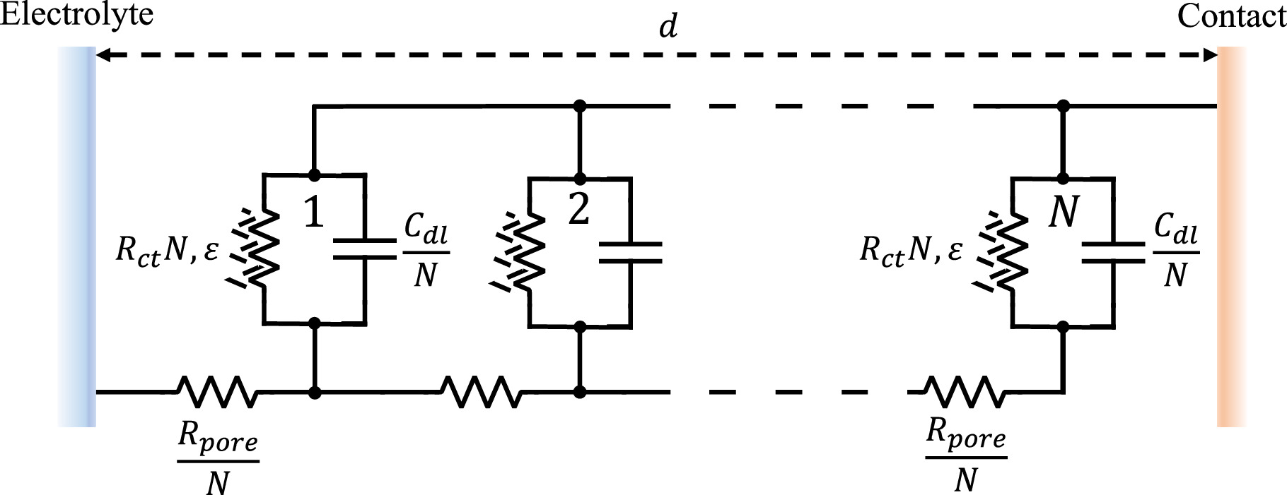
Figure 4. Transmission line representation of a porous electrode under weakly nonlinear conditions.
Download figure:
Standard image High-resolution imageSubstituting Eq. 6 into Eq. 14, and separating into first and second harmonic terms, again ignoring any higher-order terms, we find a first harmonic governing equation that is identical to the Paasch model (in the limit of zero solid resistivity),

with boundary conditions dictated by the current excitation conditions imposed at the current collector and electrolyte edge of the porous electrode,

and

The second harmonic governing equation at twice the excitation frequency ( ) is written

where we note the non-homogeneous term involving  requires the solution to Eq. 15. The homogeneous boundary conditions for the second harmonic are

and

where Eqs. 16b and 16c ensure that no second harmonic current exists at the current collector or bulk electrolyte boundary. This is a requirement in our impedance formulation because the excitation current has a single frequency, as in Eq. 5. However, the inhomogeneous term in Eq. 16a will generate internal second harmonic currents within the electrode interfaces when charge transfer is asymmetric, i.e., 
The solution of Eq. 15 is,

with the parameter

The linear EIS response for the weakly nonlinear porous electrode is found by taking Eq. 17 at the electrolyte interface ( ) and dividing by the current excitation amplitude, i.e.,

which is identical to the linear Paasch model in the limit of zero solid resistivity.
Equation 17b shows there are two relevant time constants in this porous electrode formulation, yielding two dimensionless frequencies,  and
and  The ratio between these frequencies (
 ) dictates how accessible the electrode pore structure is to current, namely, if it is a 'thin' uniformly accessible electrode (
 ), a "thick" electrode with a poorly accessible interfacial area (
 ), or somewhere in-between. The D.C. limit for the electrode impedance makes the implications of 'thin' or "thick" limits clearer on the width of the impedance arc:

The solution for Eq. 16a is


where

and

Setting Eq. 20a to its value at  the electrolyte boundary, and dividing by
  yields the 2nd-NLEIS response:


The functional forms of  and
and  suggest the 2nd-NLEIS response shares the same dimensionless frequencies as the linear system, namely,
  and
and  The magnitude for the 2nd-NLEIS spiral is set by the D.C. limit,


Figure 5 shows the Nyquist plots for the first harmonic (linear) EIS response given by Eq. 18 and the 2nd-NLEIS response given by Eq. 21 for a "thick" porous electrode where  The first harmonic response shown in Fig. 5a is characterized by a 'semi-teardrop' shape that is characteristic for thick electrodes with poor utilization of internal interfacial area. In the thick electrode limit, the frequency at the top of the EIS curve (maximum imaginary impedance) is
  Though not shown, 'thin' porous electrodes (
 ) retain the classic shape of a Randles semi-circle except at extremely high frequencies. The 2nd-NLEIS response shown in Fig. 5b has a spiral-like character akin to the weakly nonlinear Randles circuit, but with subtle differences in shape. An example of the subtle shape difference is that the 2nd-NLEIS curves in Fig. 5b only traverse two of the four Nyquist plot quadrants, whereas the Randles case in Fig. 2b had a three-quadrant spiral. As is always true for the 2nd-NLEIS, the half-cell response is proportional to the charge transfer asymmetry parameter and has a null response for symmetric charge transfer.

Figure 5. Example Nyquist plots for the weakly nonlinear response of a porous electrode with various charge transfer asymmetry parameters
 : (a) First harmonic (linear) EIS and (b) 2nd-NLEIS. The EIS response in (a) does not depend on
 . Arrows show the direction of increasing frequency with markers for 1 mHz (Δ), 100 mHz (∇), 10 Hz (□), and
  (○). The parameters used to compute the curves,
 and
and  are characteristic of a thick electrode with poorly accessible internal surface area.
Download figure:
Standard image High-resolution imageWeakly nonlinear diffusion impedance contributions to planar interfaces and porous electrodes
Diffusion dynamics in the solid or electrolyte phase of an electrochemical system can give rise to a weakly nonlinear Warburg-like diffusion impedance. Here we expand the analysis above to include solid-state bounded diffusion in the nonlinear Randles and porous electrode impedance responses. The archetypical problem considered here involves Li-ion insertion materials, where the equilibrium potential is a function of the concentration of lithium ions inserted into the solid electrode (denoted  ). A Taylor series expansion can be used to define the second order processes that describe the nonlinear oscillating equilibrium potential (
 ) of a fully relaxed non-hysteretic system,

where  is the oscillating concentration of inserted ions at the solid interface,
  and
and  are the slope and curvature of the equilibrium potential at the given state of charge (SoC) for the insertion material. To be consistent with prior results and the two-term expansion in Eq. 23, the weakly nonlinear solid state surface concentration fluctuations are expected to follow

where  and
and  are the first and second harmonic coefficients for the fluctuating insertion concentrations at the solid surface. Substituting Eqs. 24 into 23 and ignoring higher harmonics yields the weakly nonlinear oscillating equilibrium potential:


An oscillating faradaic current of the form

is consistent with our prior solutions for both planar and porous electrodes, even though the total current represented by Eq. 5 has no second harmonic component entering or leaving the electrode. The transfer function relating oscillating surface concentration to oscillating faradaic current is known as the diffusion impedance ( ), which we write as
33
), which we write as
33

and

Inserting Eq. 27 into Eq. 25 produces a compact form of the oscillating equilibrium potential


where we have defined a new differential voltage parameter  (
( )
)

that scales with the curvature of the open circuit potential at a given SoC. Charge transfer-driven diffusion nonlinearities occur at frequencies relevant to diffusive timescales set via  Expressions for the bounded diffusion impedance
  have been calculated for a variety of insertion material geometries and are summarized in Table I.
34–36
have been calculated for a variety of insertion material geometries and are summarized in Table I.
34–36
Table I. Bounded diffusion impedance for different insertion material geometries. The diffusion timescale  (
( ) is tied to the insertion material characteristic dimension
  and inserted ion diffusion coefficient
  . Bounded diffusion impedance scales with
  where
where  is the interfacial area of the electrode. The functions
  and
and  denote the modified Bessel functions of zero and first order, respectively.
| Planar | Cylindrical | Spherical | |
|---|---|---|---|

|

|

|

|
The first and second harmonic faradaic current modulations can be found through algebraic manipulation of Eqs. 1, 6, 26, and 28 to identify the coefficients multiplying  that is,

and, likewise, the coefficient multiplying  is:
is:

These expressions hold for both the planar and the porous electrode.
Weakly nonlinear response of a planar insertion electrode with bounded solid diffusion
Equation 3 provides the template for treating a weakly nonlinear planar electrode when faradaic charge transfer is accompanied by diffusion of inserted ions, that is, when Eqs. 28 and 30 are used with Eq. 3. The resulting nonlinear equivalent circuit diagram is represented by Fig. 6.
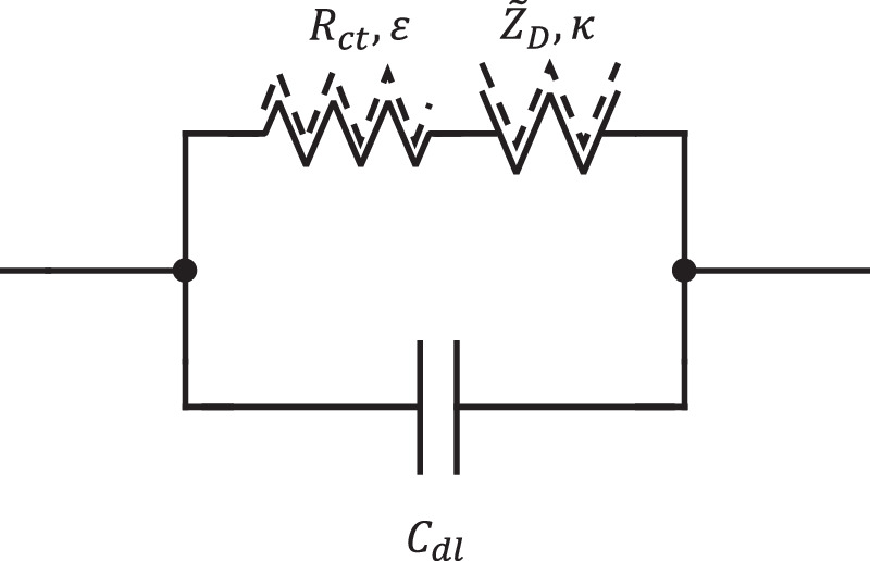
Figure 6. Equivalent circuit representation for a planar electrochemical interface with weakly nonlinear representation of charge transfer and the accompanying diffusive transport processes.
Download figure:
Standard image High-resolution imageSubstituting Eqs. 6, 28
, and 30 into Eq. 3 followed by algebraic manipulation and separation of equations into first and second harmonics produces expressions for  and
and  Equation 7 is used with the
  solution to write the first harmonic (linear) EIS response

while solutions to  are used with Eq. 8 to write the second harmonic NLEIS response

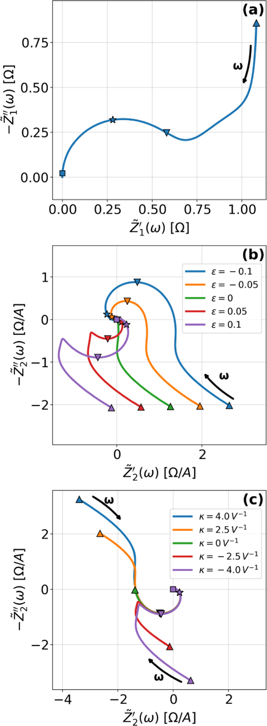
Equations 31 and 32 enable the simulation of the full spectrum linear EIS and 2nd-NLEIS response for a planar thin film of insertion material on a current collector substrate. Figure 7a shows a Nyquist plot for linear EIS, where a Randles charge transfer semi-circle at higher frequencies is seen to merge into a 45-degree diffusive impedance at intermediate frequencies and, ultimately, the chemical capacitance of the bounded thin film is observed at sufficiently low frequencies. The corresponding 2nd-NLEIS response is explored as a function of the charge transfer asymmetry parameter ( ) in Fig. 7b and as a function of the voltage curvature parameter (
 ) in Fig. 7c. Figure 7b shows the same three-quadrant 2nd-NLEIS charge transfer spiral as the weakly nonlinear Randles circuit presented in Fig. 2, but as the frequency becomes low enough to activate diffusive processes, the weakly nonlinear bounded diffusion impedance terms in Eq. 32 becomes apparent. Figure 7c shows the effect of
  on the nonlinear second harmonic response. As shown in the Nyquist plot, the direction and magnitude of the weakly nonlinear diffusion response are governed by the
  For the parameters shown here, the case of
  equal to zero is close to the pure charge transfer behavior with Eq. 32 reverting to the pure charge transfer DC limit. One could imagine when the charge transfer time scale and diffusion time scale are comparable to each other, a larger deviation from pure charge transfer reaction might displayed even when
  is zero. The direction-sensitive features of 2nd-NLEIS — where realistic charge transfer and diffusion parameters can produce signals in all four quadrants of a Nyquist plot — significantly boost the mathematical discriminating power of 2nd-NLEIS over conventional one-quadrant linear EIS. We discuss this parameter sensitivity as an especially important feature for full-cell studies in the Implications and Concluding Remarks section.

Figure 7. Example Nyquist plots for the weakly nonlinear response of a planar thin film insertion electrode with varying charge transfer asymmetry (
 ) and differential voltage (
 ) parameters. (a) First harmonic (linear) EIS is independent of
 and
and  (b) The 2nd-NLEIS spectrum as a function of
 for
for  (c) The second harmonic NLEIS spectrum as a function of
  for
for  Arrows show the direction of increasing frequency with markers for 1 mHz (Δ), 100 mHz (∇), 10 Hz (□), and
  (*). The parameters used to compute the curves are

 and
and 
Download figure:
Standard image High-resolution imageWeakly nonlinear response of a porous insertion electrode with bounded solid diffusion
Equation 4 is the starting point for describing a porous insertion electrode with solid-state diffusive transport. The corresponding weakly nonlinear equivalent circuit representation of such a porous electrode is shown in Fig. 8.

Figure 8. Equivalent circuit representation of a weakly nonlinear porous electrode with diffusive transport limitation under the weakly nonlinear condition.
Download figure:
Standard image High-resolution imageSubstituting Eqs. 5, 28 , and 30 into Eq. 4 and separating terms into first and second harmonic equations, while ignoring higher order harmonics, yields the first harmonic (linear) governing equation:

with identical boundary conditions to Eq. 15b and 15c. The solution to Eq. 33 is identical to Eq. 17a, but with Eq. 17b replaced by the diffusion impedance modified parameter

yielding the linear EIS impedance

Formulating the second harmonic porous electrode response when solid state bounded diffusion effects are included yields a governing equation and boundary conditions identical in form to Eq. 16a, resulting in a solution having an identical form to Eq. 20a and 2nd-NLEIS response


with the diffusion impedance modified parameters

and

being the only differentiating factor between Eqs. 36 and 21.
Equations 35 and 36 enable the simulation of the full spectrum linear EIS and 2nd-NLEIS response for a porous insertion electrode on a current collector substrate. Figure 9a shows a Nyquist plot for linear EIS, where a typical "thick" porous electrode charge transfer teardrop shape is seen at frequencies above 100 mHz, akin to what is seen in Fig. 5a without any diffusion effects. At frequencies below 100 mHz, the effect of diffusive transport becomes evident as the 45-degree diffusive impedance transitions to a chemical capacitance behavior in the bounded thin film at the lowest frequencies shown. Here we assume the porous electrode was built from planar (platelet-like) particles, hence the "planar" functional form is used for the diffusion impedance in Table I. The corresponding 2nd-NLEIS response is explored as a function of the charge transfer asymmetry parameter ( ) in Fig. 9b and as a function of the potential curvature parameter (
 ) in Fig. 9c. Figure 9b shows the same two-quadrant 2nd-NLEIS charge transfer spiral at frequencies above 100 mHz as we saw in Fig. 5, but as the frequency becomes lower, the weakly nonlinear bounded diffusion impedance terms in Eqs. 36 and 37 becomes apparent. Figure 9c shows the effect of
  on the scaling and quadrants where the low frequency nonlinear second harmonic diffusion processes appear. In contrast to the planar electrode, there is a distinct weakly nonlinear diffusion response for the porous electrode even when
  equals to zero, which is primarily due to the inhomogeneity of the current distribution with the presence of pore electrolyte.

Figure 9. Example Nyquist plots for the weakly nonlinear response of a porous insertion electrode with varying charge transfer asymmetry (
 ) and differential voltage (
 ) parameters. (a) First harmonic (linear) EIS is independent of
  and
and
 (b) The 2nd-NLEIS spectrum as a function of
 for
for  (c) The 2nd-NLEIS spectrum as a function of
  for
for  Arrows show the direction of increasing frequency with markers for 1 mHz (Δ), 100 mHz (∇), 10 Hz (□), and (○). The particles making up the porous insertion electrode are assumed to be planar (platelet-like) particles (Table I), with the parameters used


 and
and 
Download figure:
Standard image High-resolution imageImplications and Concluding Remarks
Signal parity and second harmonic NLEIS (2nd-NLEIS) for two-electrode cells
Linearization used in traditional EIS techniques leads to half-cell model degeneracy with both physics-based models 12 or equivalent circuit models. 11 The challenge of half-cell degeneracy is compounded when analyzing two-electrode cells. The origin of this compounding impact is that a two-electrode cell has an EIS response that is the sum of half-cell EIS signals; thus, two-electrode linear EIS is a "positive parity" signal owing to the additive trait of half-cells. This positive parity trait makes it even more difficult to assign the physicochemical contributions to the EIS signal of a particular electrode.
2nd-NLEIS is effective at addressing the challenge of model degeneracy in half-cell measurements. 12 Perhaps more importantly, the two-electrode 2nd-NLEIS signal arises from the difference between the half-cell 2nd-NLEIS responses; 22 thus, two electrode 2nd-NLEIS is a "negative parity" signal owing to subtractive traits of half-cells. The complementary parity between EIS and 2nd-NLEIS, when analyzed with a common physics-based model, makes assigning half-cell physicochemical processes from two-electrode measurements much more feasible.
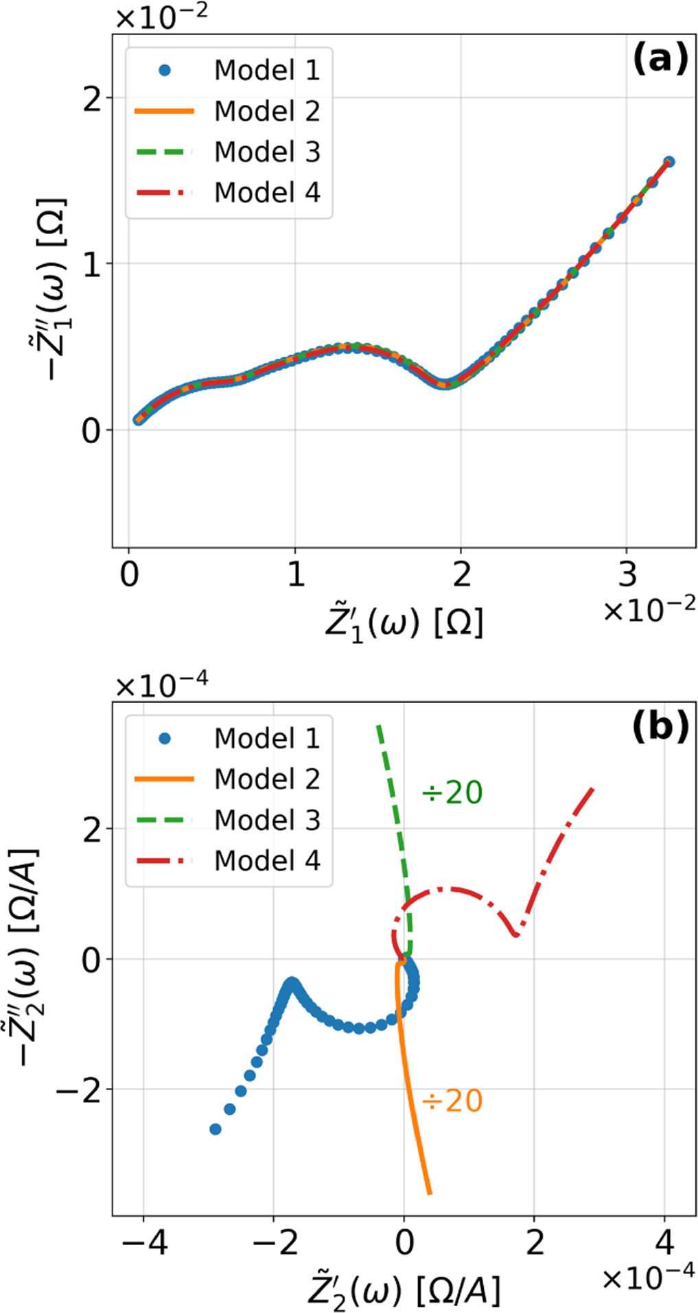
To demonstrate the importance of using complementary parity signals to assign physicochemical process, we use the half-cell modeling above to build four different two-electrode models that each fairly closely represent the linear EIS response from two-electrode battery data presented by Murbach et al. 22 The four distinct models were built by simply "swapping" charge transfer and diffusion-related physicochemical parameters systematically among the positive and negative electrodes, creating the four parameter sets summarized in Table II. Figure 10a shows the simulated Nyquist plots for each two-electrode linear EIS model. The positive parity additive response makes it difficult to assign the charge transfer and diffusion properties to one electrode or another. Though not truly degenerate (there are subtle differences among the four cases), the two-electrode EIS responses are practically indistinguishable. The Nyquist plots for the four corresponding two-electrode 2nd-NLEIS models are shown in Fig. 10b. In contrast to Fig. 10a, each negative-parity NLEIS model for the two-electrode cells has a highly distinct response that is sensitive to the assignment of specific physicochemical parameters to specific electrodes. In short, the complementary parity between linear EIS and 2nd-NLEIS in a two-electrode configuration provides the discriminating power needed to assign half-cell processes in a two-electrode configuration that lacks a separate reference measurement.
Table II. Parameters of first and second harmonic impedance simulation for four nearly degenerated linear first harmonic models and their corresponding nonlinear second harmonic models.
| Physicochemical Parameter | Model 1 | Model 2 | Model 3 | Model 4 | ||
|---|---|---|---|---|---|---|
| Cathode | Charge Transfer |
![${R}_{{pore},c}\,[{\rm{\Omega }}]$](https://content.cld.iop.org/journals/1945-7111/170/12/123511/revision3/jesad15caieqn249.gif)
|

|

|

|

|
![${R}_{c}\,[{\rm{\Omega }}]$](https://content.cld.iop.org/journals/1945-7111/170/12/123511/revision3/jesad15caieqn254.gif)
|

|

|

|

| ||
![${C}_{c}\,[F]$](https://content.cld.iop.org/journals/1945-7111/170/12/123511/revision3/jesad15caieqn259.gif)
|

|

|

|

| ||
| Diffusion |
![${A}_{W,c}\,[{\rm{\Omega }}]$](https://content.cld.iop.org/journals/1945-7111/170/12/123511/revision3/jesad15caieqn264.gif)
|

|

|

|

| |
![${\tau }_{c}[s]$](https://content.cld.iop.org/journals/1945-7111/170/12/123511/revision3/jesad15caieqn269.gif)
|

|

|

|

| ||
| NLEIS Parameters |
![${\kappa }_{c}\,[{V}^{-1}]$](https://content.cld.iop.org/journals/1945-7111/170/12/123511/revision3/jesad15caieqn274.gif)
|

|

|

|

| |
![${\varepsilon }_{c}[]$](https://content.cld.iop.org/journals/1945-7111/170/12/123511/revision3/jesad15caieqn279.gif)
|

|

|

|

| ||
| Anode | Charge Transfer |
![${R}_{{pore},a}\,[{\rm{\Omega }}]$](https://content.cld.iop.org/journals/1945-7111/170/12/123511/revision3/jesad15caieqn284.gif)
|

|

|

|

|
![${R}_{a}\,[{\rm{\Omega }}]$](https://content.cld.iop.org/journals/1945-7111/170/12/123511/revision3/jesad15caieqn289.gif)
|

|

|

|

| ||
![${C}_{a}\,[F]$](https://content.cld.iop.org/journals/1945-7111/170/12/123511/revision3/jesad15caieqn294.gif)
|

|

|

|

| ||
| Diffusion |
![${A}_{W,a}\,[{\rm{\Omega }}]$](https://content.cld.iop.org/journals/1945-7111/170/12/123511/revision3/jesad15caieqn299.gif)
|

|

|

|

| |
![${\tau }_{a}[s]$](https://content.cld.iop.org/journals/1945-7111/170/12/123511/revision3/jesad15caieqn304.gif)
|

|

|

|

| ||
| NLEIS Parameters |
![${\kappa }_{a}\,[{V}^{-1}]$](https://content.cld.iop.org/journals/1945-7111/170/12/123511/revision3/jesad15caieqn309.gif)
|

|

|

|

| |
![${\varepsilon }_{a}[]$](https://content.cld.iop.org/journals/1945-7111/170/12/123511/revision3/jesad15caieqn314.gif)
|

|

|

|

| ||
Figure 10. Simulated Nyquist plots for (a) four nearly degenerated linear models and (b) the corresponding nonlinear second harmonic responses. The real and imaginary nonlinear second harmonic responses for models 2 and 3 are divided by 20 to place them on the same scale as the other 2nd-NLEIS responses.
Download figure:
Standard image High-resolution image
The implications for the half-cell and two-electrode cell analysis given here, when combined with our prior work on the experimental accessibility of two-harmonic measurements, is that 2nd-NLEIS is a truly complementary measurement that should be added to the EIS toolbox in order to take advantage of the discriminating power described above. To build confidence in 2nd-NLEIS based methods, adoption of the advanced quality assurance and analysis methods that have become fairly routine in the linear EIS community 9 need to be advanced to the second harmonic. A key question that underpins the efficient adoption of 2nd-NLEIS is how to systematically test that an experimental modulation is adequate to excite the second-order weakly nonlinear effects analyzed here, without over-driving the system into third-order (and higher) nonlinear processes that will distort the linear EIS signals, avoiding the need to use more sophisticated series analysis to extract any meaningful parameters (e.g., see analysis in Murbach et al.'s work 23 ). In the experiments we've reported previously, modulated voltages of roughly 10–15 mV (at frequencies that activate charge transfer and diffusion processes) appear to nicely drive second-order (two term, two harmonic) responses without overly exciting higher-order distortions. 22
Equivalent circuit representations, and further generalization
As shown above, building the second harmonic nonlinear impedance response from two-term (weakly nonlinear) expansions of interfacial and transport models creates a mathematical structure that is consistent with the parallel and series circuit element additivity rules of linear circuits. We formally introduced the consequences of two-term expansions of the Butler-Volmer charge transfer model and solid-state bounded diffusion. In contrast, we chose a constant coefficient Helmholtz model for the double layer which avoids nonlinear contributions to the non-faradaic current; this allowed us to show that mixing linear and nonlinear elements is easily accomplished and it also aligned the work here with previous nonlinear pseudo-2-D modeling of porous insertion electrodes. 23
For completeness, we note that more general descriptions of the electrochemical double layer require a replacement of Eq. 2, given that interfacial capacitance is no longer a constant:

Most double-layer models represent the double layer capacitance as a function of interfacial potential  Because 2nd-NLEIS perturbs the interface from its equilibrium state with small but finite modulations, it is reasonable to use a two-term Taylor series expansion for the capacitance, yielding a universal "local" form for the capacitance of

where  is the capacitance of the interface at the equilibrium potential and
  is a model-dependent nondimensional constant. The combination of Eqs. 38a and 38b creates a direct replacement for Eq. 2 that introduces second order nonlinearity into the governing equation for non-faradaic currents. Had Eq. 38 been used throughout this paper, the linear EIS response would be unchanged, but the 2nd-NLEIS response would have many extra terms and an extra parameter
  in the solutions for each specific case studied.
The selection of a particular double layer structure yields a detailed interpretation of the model-dependent constant  For example, a Gouy-Chapman double layer with monovalent ions yields
 ![${\rm{\Theta }}=0.5\,{\rm{* }}\,\tanh \left[0.5f\left({E}_{n}-{E}_{{pzc}}\right)\right],$](https://content.cld.iop.org/journals/1945-7111/170/12/123511/revision3/jesad15caieqn324.gif) where
where  is the potential of zero charge (PZC) for the interface. For the Gouy-Chapman model, interfacial capacitance has a local minimum at the PZC with
  resulting in no 2nd-NLEIS contribution from the double layer. More broadly, nonlinear double layer contributions to 2nd-NLEIS spectra are likely to only be important at highly polarizable interfaces and at high frequencies where faradaic charge transfer contributions are negligible. In short, though not used here, non-faradaic currents can contribute to 2nd-NLEIS through the second-order nonlinearity generated by a non-constant double layer capacitance. The form of the contribution, Eq. 38b, is universal but the interpretation of the new nonlinear parameter
  is dependent on the interfacial structure of models. For electrochemical energy systems we mostly study, facile charge transfer is a key feature of the electrochemical interface, so the impact of weak double-layer nonlinearity is diminished.
Shown in Table III is a visual representation of the linear and two-term weakly nonlinear elements that underpin all the analysis above. We adapt traditional linear EIS circuit element representations and add a parallel dashed line to represent the second-order nonlinear form of each linear circuit element. Adding a parallel dashed line conveys the use of a two-term expansion to represent the second-order nonlinear electrochemical processes being analyzed. As shown in Figs. 3, 4, 6, and 8, one can mix and match linear and second-order impedance elements to visualize the mix of physical assumptions that underpin the linear and second harmonic response of the corresponding Nyquist plots. Such development of visual representation emphasizes the ability to substitute linear circuit elements with appropriate nonlinear element circuits to take advantage of the existing TLM models 29–32,37,38 in describing different electrochemical processes, while obtaining additional insights about reaction kinetics and thermodynamics with the complementary 2nd-NLEIS analysis.
Table III. Circuit element representations for the first and second harmonic impedance response when a two-term expansion is used to represent a nonlinear electrochemical process.
| Circuit Elements | Linear EIS | 2nd Harmonic NLEIS |
|---|---|---|
| Resistor |

|

|
| Capacitor |
|
|
| Diffusion element |

|

|
To conclude, second harmonic nonlinear electrochemical impedance spectroscopy (2nd-NLEIS) is a powerful tool for probing complementary information to traditional electrochemical impedance spectroscopy (EIS), extracting meaningful non-linear contributions to charge transfer, mass transport, and thermodynamics of the electrochemical systems. However, the application of the 2nd-NLEIS has been hampered by the lack of simple models able to extract meaningful parameters. To resolve this problem, we systematically developed simple physics-based models for planar electrochemical interfaces and porous electrodes that are governed by a Helmholtz double layer, Butler–Volmer kinetics, and solid-state bounded Fickian diffusion. The limiting cases and dependences of the second harmonic impedance response on charge transfer asymmetry and thermodynamics are explored. The importance of using the complementary parity between linear EIS and 2nd-NLEIS as a strategy to separate half-cell parameters for two-electrode measurements is discussed. For completeness, the nonlinear double-layer response for non-faradaic current is briefly introduced for the interested reader. Lastly, we try to depict a sensible visual representation of second order nonlinear circuit elements as a shorthand way to identify the mathematical underpinning and structure of the analysis, helping bridge the gap between model-based analysis, experiments, and the intuition needed for the physical interpretation of EIS and 2nd-NLEIS data.
Acknowledgments
This research was made possible through the support of Yuefan Ji with State of Washington proviso funding for Clean Energy Institute Graduate Fellowships and the Boeing-Sutter endowment for excellence in engineering. The authors thank David Larsen and McCrae Leith for preliminary explorations that helped shape the direction of this work.