
Abstract
This study applies, tests, and compares comprehensive surrogate-based optimization techniques to optimize the performance of polymer electrolyte membrane fuel cells (PEMFCs). Moreover, parametric cases considering four important design variables, i.e., gas diffusion layer thickness ( ), channel depth (
 ), channel width (
 ), and land width (
 ), are defined using the latin hypercube sampling technique under reasonable constraint conditions. Multidimensional, two-phase PEMFC model simulations are performed to generate the training and test data under these design conditions. Three famous surrogate models, i.e., response surface approximation (RSA), radial basis neural network (RBNN), and kriging (KRG), are employed to construct objective functions for the PEMFC cell voltages operating in the galvanostatic mode, and their accuracies are tested and compared using root mean square error and adjusted R-square. The surrogates are then linked to stochastic optimization algorithms, i.e., genetic algorithm and particle swarm optimization, to determine the optimal design points. A comparative study of these surrogates reveals that the KRG model outperforms the RBNN and RSA models in terms of prediction capability. Furthermore, the PEMFC model simulations at the optimal design points clearly demonstrate that performance improvements of around 56–69 mV at 2.0 A cm−2 are achieved with the optimum design values compared to typical PEMFC design conditions.
Export citation and abstract BibTeX RIS

This is an open access article distributed under the terms of the Creative Commons Attribution 4.0 License (CC BY, http://creativecommons.org/licenses/by/4.0/), which permits unrestricted reuse of the work in any medium, provided the original work is properly cited.
List of symbols
| a | Ratio of active surface area per unit electrode volume, m2 m−3 |
| A | Area, m2 |
| c | Center of input sample data |
| C | Molar concentration of species, mol/m3 or acceleration factor |

| Correlation value |
| d | Number of input variables |
| D | Species diffusivity, m2/s |
| E | Activation energy, kJ/mol |
| EW | Equivalent weight of a dry membrane, kg/mol |

| Actual response function |
| F | Faraday's constant, 96,487 C mol−1 |
| G | Global best |
| h | Activation function |
| i0 | Exchange current density, A cm−2 |
| I | Operating current density, A cm−2 |
| j | Transfer current density, A cm−3 |
| k | Thermal conductivity, W/m·K, or Relative permeability |
| K | Hydraulic permeability, m2 |
| L | Least square function or Loading of particles, mg/m2 |
| n | Number of electrons transferred in the electrode reaction |
| N | Number of training points |
| MW | Molecular weight, kg mol−1 |
| MSE | Mean squared error |
| P | Pressure, Pa, or Particle personal best |
| p | Number of weight coefficients in each second-order equation |
| q | Mating rate |
| r | Radius of particles, m |
| Q | Number of the sampling points |
| RMSE | Root mean squared error |

| Correlation coefficient |
| s | Liquid saturation |
| S | Source term in the transport equation or Population |
| SSE | Squared sum error |
| t | Iteration time step |
| T | Temperature, K |

| Fluid velocity and superficial velocity in a porous medium, m/s |
| V | Particle velocity |

| Input variable |

| Observed response |

| Predicted response |
| z | Transport resistance coefficient |
| Greek symbols | |
| α | Transfer coefficient |

| Weight coefficient |
| γ | Reaction order |
| δ | Thickness, m |
| ε | Volume fraction or Error |
| η | Surface overpotential, V |

| Contact angle of the gas diffusion layer |

| Estimated mean value from training data set distribution |
| κ | Proton conductivity, S m− |
| ϕ | Phase potential, V |
| ρ | Density, kg/m |
| σ | Electronic conductivity, S m−, or Variance of input training data |
| τ | Viscous shear stress, N/m2 |
| ξ | Stoichiometry flow ratio |

| Correlation matrix between training point and unknown point |

| Correlation matrix between whole training points |
| Ω | Oxygen transport resistance |
| Superscripts | |
| c | Catalyst coverage coefficient |
| eff | Effective |
| g | Gas |
| l | Liquid |
| mem | Membrane |
| ref | Reference value |
| Subscripts | |
| a | Anode |
| c | Cathode |
| CL | Catalyst layer |
| e | Electrolyte |
| ch | Gas channel |
| gdl | Gas diffusion layer |
| i | Species |
| in | Channel inlet |
| int | Interface |
| mem | Membrane |
| Pt | Platinum |
| s | Solid, surface |
| T | Temperature |
| u | Momentum equation |
| w | Water |
| 0 | Initial conditions or standard conditions, i.e., 298.15 K and 101.3 kPa (1 atm) |
Fossil fuel is key to the growth and development of all countries. When fossil fuels are burned, carbon dioxide  is released, which is a major contributor to global climate change. The
  release into the atmosphere causes local air pollution, which is annually said to be a major cause of premature deaths.
1
Hence, an energy resource that is a low carbon source, readily available, and pollution free is immediately required. Renewable power resources are deemed as proper candidates for restoring fossil fuels. A renewable power source that will beget an era of minimal pollution is hydrogen fuel cells. A fuel cell is an electrochemical cell that generates electrical energy from an electrochemical reaction, and polymer electrolyte membrane fuel cells (PEMFCs) are the most promising fuel cells. During the past decade, PEMFCs have emerged as the favored technology for power generation and auto transport. They are compact, clean, and can be operated at low temperatures (less than 100 °C).
release into the atmosphere causes local air pollution, which is annually said to be a major cause of premature deaths.
1
Hence, an energy resource that is a low carbon source, readily available, and pollution free is immediately required. Renewable power resources are deemed as proper candidates for restoring fossil fuels. A renewable power source that will beget an era of minimal pollution is hydrogen fuel cells. A fuel cell is an electrochemical cell that generates electrical energy from an electrochemical reaction, and polymer electrolyte membrane fuel cells (PEMFCs) are the most promising fuel cells. During the past decade, PEMFCs have emerged as the favored technology for power generation and auto transport. They are compact, clean, and can be operated at low temperatures (less than 100 °C).
However, the growth and development of PEMFCs are hindered by high costs, weight, and volume. The PEMFC performance is influenced by several parameters, such as the design of cell components, operating pressure, operating temperature, and humidification of the inlet gases. To achieve maximum cell performance, the effects of these parameters on the fuel cell operation need to be understood.
Recently, several experiments and numerical simulations have been performed on PEMFCs focusing on various operating parameters that influence their performance, including operating temperatures, humidification, gas flow rate, and operating pressures. Wang et al. 2 analyzed the effects of parameters such as operating temperatures, humidification, and operating pressures. Their results showed that the fuel cell performance increases with pressure due to an increase in the exchange current density and reactant gas partial pressure. Suleyman et al. 3 applied the Taguchi method for experimental designs to determine the optimum PEMFC working conditions for obtaining the maximum power density. The optimization results showed that pressure and humidification temperatures are effective parameters. Yan et al. 4 investigated the impacts of operating conditions such as inlet gas flow rate, humidification temperature, and operating cell temperature for a PEMFC with conventional and interdigitated flow field. The experimental results showed that the cell performance improves when the inlet gas flow rate and humidification temperature at the cathode are increased.
In addition to the aforementioned operating factors, other parameters affect the fuel cell performance. Lee et al. 5 conducted a parametric study of channel designs and their effects on PEMFC performance using computational fluid dynamics (CFD) techniques. The channel height, width, ratio of channel land, and gas diffusion layer (GDL) thickness were considered, and their effects on performance were examined. Their results showed that there is a trade-off between the performance and pressure drop for different design parameter combinations in the system, and these effects have to be considered during PEMFC system design. Zhang et al. 6 conducted studies on the effect of different land widths. They determined that decreasing the land width and increasing the inlet flow rates improved the fuel cell performance. Muthukumar et al. 7 conducted a numerical study to analyze the effects of different land to channel widths on PEMFCs. The polarization and power density curves showed that small channel widths and rib dimensions are suitable to obtain high current and power density values. Lin and Prassana et al. 8,9 analyzed the effects of GDL thickness on the PEMFC performance. They suggested that a thin GDL would improve the gas diffusion rates, but it is susceptible to mechanical failure. This clearly shows that there is an optimum thickness for improved cell performance. Liu et al. 10 developed a PEMFC mathematical model and used it to optimize the PEMFC channel dimensions. The obtained results were experimentally tested to determine the maximum power density in the cell. They found that relatively small flow channel and rib width are preferred to afford high power density.
The above discussed literature survey reveals the importance of the effects of operational and design parameters in PEMFC operation and the need for optimizing these parameters. Moreover, improving cell performance and reducing manufacturing costs are the most important steps in the growth of the fuel cell industry. The development and growth of PEMFCs can be significantly optimized by improving the mathematical and numerical modeling to determine more efficient ways of generating the fuel cells. Over the last decades, commercially available CFD and mathematical models have evolved. 11–17 However, they are often in a complex form, and the estimation of the PEMFC performance requires a significant amount of computational turnaround time and resources. One way of overcoming this burden is to construct computationally cheaper models, known as surrogates or metamodels, that can very closely represent the simulation models.
Data-driven surrogates have been developed, tested, and used in PEMFC applications. 15–18 Well-known surrogates include response surface approximation (RSA), radial basis neural network (RBNN), kriging (KRG), support vector machines (SVM), and artificial neural networks. Kanani et al. 19 employed a quadratic RSA surrogate model to determine the maximum power in a single-cell serpentine PEMFC. Experimental data and the design of experiment (DOE) approach were employed to build the dataset. To determine the maximum power at the optimal operating condition, the RSA optimizer was employed. Wang et al. 20 found the maximum power density for a PEMFC by employing a novel artificial-intelligence-based SVM surrogate model with a radial basis function (RBF) activation function. The surrogate model was constructed with a CFD dataset of 65 points, with 50 random points for training and 15 points for testing. Then, the genetic algorithm (GA) was adopted to investigate the optimal catalyst layer (CL) composition. Xing et al. 21 optimized CL design variables using the KRG-based surrogate model where the sample data were generated through CFD simulations. Optimum CL design parameters were determined for specific operating voltage ranges and a fixed operating voltage. Furthermore, to determine the influence of each design parameter on the objective function, the sobol global sensitivity analysis based on the Monte Carlo technique was applied. Cheng et al. 22 proposed an optimization methodology with the experimental database to find the optimal operational parameters using the RBF neural network surrogate model coupled with GA. The effects of the operational parameters on the PEMFC performance were verified with the DOE and Taguchi orthogonal array methods. Moreover, the cross-validation procedure from significant factors based on the analysis of variance was employed to verify the meta model accuracy.
A literature review revealed that different surrogate modeling techniques can be employed to achieve the prediction level of multidimensional complex numerical fuel cell models with acceptable accuracy and low processing time. Additionally, key fuel cell design parameters can be effectively optimized by linking the surrogates with a cheap optimization algorithm, thereby saving valuable time and cost. Herein, we attempt to optimize key fuel cell design parameters for the cathode GDL and flowfield using a CFD/finite element method simulation-based optimization approach. First, parametric cases with different cathode GDL and flowfield dimensions are defined using the latin hypercube sampling (LHS) technique under reasonable constraint conditions. Then, a multiscale, two-phase, three-dimensional (3D) PEMFC model developed in our previous studies 23–26 is applied to various PEMFC geometries corresponding to the parametric cases. Particular emphasis is placed on considering the GDL compression/intrusion effects via fluid-structure interaction (FSI) simulations since they substantially influence the transport characteristics and cell performance. 27 For comparison, three famous surrogate models, i.e., RSA, RBNN, and KRG, are constructed in-house using MATLAB R2021a and then trained based on the fuel cell model simulation data. These surrogate models are linked to stochastic optimization algorithms, such as GA and particle swarm optimization (PSO), to determine the optimal cathode GDL and flowfield design parameters. Finally, the accuracy of these optimum values is further evaluated via comprehensive PEMFC model simulations to probe the validity of such fuel cell optimization methodology.
Numerical PEMFC model
A 3D, multi-scale, two-phase PEMFC model is used for this optimization study. It is based on the multiphase mixture (M2) formulation proposed by Wang and Cheng. 28 The model considers various PEMFC components, including the membrane, CLs, microporous layers, GDLs, and bipolar plates (BPs). The 3D PEMFC model has been previously validated against experimental polarization curves measured under various cell designs and operating conditions. 24 Furthermore, the influence of uneven GDL deformation during compression (due to clamping) has been considered in the 3D PEMFC model specifically wherein the zone in contact with the lands of bipolar plates undergoes compression and the GDL beneath the flow channels is uncompressed and pushed into the channel region (intrusion). Since the model used herein is similar to that described in our previous study, 11,23,26,29 the model assumptions, governing equations, boundary conditions and numerical implementation of the PEMFC model featured using commercial CFD software, ANSYS Fluent (ANSYS Inc., USA) are briefly summarized in the present manuscript and can be referred below.
Model assumptions
This numerical study is based on the following specific assumptions
- 1.The operation pressure is low, and hence, ideal gas mixtures are considered in the gas phase.
- 2.The flow velocity is low and laminar.
- 3.The gravitation effect is negligible.
- 4.The effect of immobile liquid saturation in the porous region is negligible.
Governing equations and source terms
The PEMFC model considered herein is governed by five principles of conservation: mass, species, charge, momentum, and thermal energy. The above-stated equations are coupled with source terms related to electrochemical reactions in the anode (hydrogen oxidation reaction; HOR) and cathode (oxygen reduction reaction; ORR). The governing equations and source terms are listed in Table I and II, respectively, for reference.
Table I. PEMFC model: governing equations.
| Governing equations | ||
|---|---|---|
| Mass |

| (37) |
| Momentum |
| (38) |
| Species | Flow channels and porous media: | |
![$\begin{array}{l}{\rm{\nabla }}\cdot \left({\gamma }_{i}\rho {m}_{i}\vec{u}\right)={\rm{\nabla }}\cdot \left[{\rho }^{g}{D}_{i}^{g,eff}{\rm{\nabla }}\left({m}_{i}^{g}\right)\right]\\ \,+{\rm{\nabla }}\cdot \left[\left({m}_{i}^{g}-{m}_{i}^{l}\right){\vec{j}}^{l}\right]+{S}_{i}\end{array}$](https://content.cld.iop.org/journals/1945-7111/169/1/014511/revision2/jesac492fieqn21.gif)
| (39) | |
| Water transport in membrane: | ||
| (40) | |
| Charge | Proton transport: | |
| (41) | |
| Electron transport: | ||
| (42) | |
| Energy |
| (43) |
Table II. PEMFC model: Source/sink terms.
| Description | Expressions | |
|---|---|---|
| Momentum | Porous media |

|
| Species | H2 in anode CL |
![${{\rm{S}}}_{{H}_{2},a}=\left[-\displaystyle \frac{j}{2F}\right]{{\rm{M}}}_{{H}_{2}}$](https://content.cld.iop.org/journals/1945-7111/169/1/014511/revision2/jesac492fieqn27.gif)
|
| O2 in cathode CL |
![${{\rm{S}}}_{{O}_{2},c}=\left[\displaystyle \frac{j}{4F}\right]{{\rm{M}}}_{{O}_{2}}$](https://content.cld.iop.org/journals/1945-7111/169/1/014511/revision2/jesac492fieqn28.gif)
| |
| Water in anode CL |
![${{\rm{S}}}_{w,a}=\left[-{\rm{\nabla }}\cdot \left(\displaystyle \frac{{n}_{d}}{F}\vec{I}\right)+\displaystyle \frac{j}{4F}\right]{{\rm{M}}}_{w}$](https://content.cld.iop.org/journals/1945-7111/169/1/014511/revision2/jesac492fieqn29.gif)
| |
| Water in cathode CL |
![${{\rm{S}}}_{w,c}=\left[-{\rm{\nabla }}\cdot \left(\displaystyle \frac{{n}_{d}}{F}\vec{I}\right)-\displaystyle \frac{j}{2F}\right]{{\rm{M}}}_{w}$](https://content.cld.iop.org/journals/1945-7111/169/1/014511/revision2/jesac492fieqn30.gif)
| |
| Energy | In anode CL |

|
| In cathode CL |
| |
| In membrane |

| |
| Charge | In CLs: |

|
Electrochemical reactions 
| ||
HOR on the anode side: 
| ||
ORR on the cathode side: 
| ||
| Transfer current | HOR in anode CL: | |
density, ![$\left[A/{m}^{3}\right]$](https://content.cld.iop.org/journals/1945-7111/169/1/014511/revision2/jesac492fieqn38.gif)
|
![$\begin{array}{l}j=\left(1-s\right)a{i}_{0,a}^{ref}{\left(\displaystyle \frac{{C}_{{H}_{2}}}{{C}_{{H}_{2},ref}}\right)}^{\displaystyle \frac{1}{2}}\,\exp \left[-\displaystyle \frac{{E}_{a}}{R}\left(\displaystyle \frac{1}{T}-\displaystyle \frac{1}{353.15}\right)\right]\\ \,\times \,\left(\exp \left(\displaystyle \frac{{\alpha }_{a}F}{RT}\eta \right)-\exp \left(-\displaystyle \frac{{\alpha }_{c}F}{RT}\eta \right)\right)\end{array}$](https://content.cld.iop.org/journals/1945-7111/169/1/014511/revision2/jesac492fieqn39.gif)
| (44) |
| ORR in cathode CL: | ||
| (45) | |
| Overpotential |

| (46) |
where 
| ||
Additionally, the kinetic, transport, and physiochemical properties of the PEMFC components are listed in Table III. The M2 model proposed by Wang and Cheng
30
is employed herein, and the mixture properties are listed in Table IV. Table V lists a set of the species' transport properties, and they are correlated to the water content  which subsequently is a function of the water activity
  31
31
Table III. Kinetic, transport, and physiochemical properties.
| Description | Value/Expression | References |
|---|---|---|
Exchange current density of HOR × ECSA per unit CL volume, 
| 1.2 × 10¹⁰ A m−3 | 24 |
Exchange current density for ORR, 
| 2.0 × 10⁻⁴ A cm−2-P−1t−1 | 11 |
Activation energy of anode, 
| 10.0 kJ mol−1 | 24 |
Activation energy of cathode, 
| 70.0 kJ mol−1 | 24 |
Transfer coefficient of HOR, 
| 1 | 25 |
Transfer coefficient of ORR, 
| 1 | 25 |
Reference H2/O2 molar concentration, 
| 40.88 mol m−3 | 25 |
Permeability of GDL/CL, 
| 1.0 × 10⁻¹²/1.0 × 10−13 m2 | 24 |
Equivalent weight of electrolyte in the membrane, 
| 1.1 kg mol−1 | 24 |
| Young's modulus of GDL | 6.16 MPa | 42 |
| Poisson ratio of GDL | 0.09 | 29 |
Faraday's constant, 
| 96,485 C mol−1 | 25 |
Universal gas constant, 
| 8.314 
| |
H2 diffusivity in the anode gas channel, 
| 1.1028 × 10⁻⁴ m2 s−1 | 25 |
H2O diffusivity in the anode gas channel, 
| 1.1028 × 10⁻⁴ m2 s−1 | 25 |
O2 diffusivity in the cathode gas channel, 
| 3.2348 × 10⁻⁴ m2 s−1 | 25 |
H2O diffusivity in the cathode gas channel, 
| 7.35 × 10⁻⁵ m2 s−1 | 25 |
Binary gas diffusivity ( ) ) | For nonporous regions | |
| (47) | |
Effective diffusivity ( ) ) | For porous regions | |

| (48) |
Table IV. Expressions used in the two-phase mixture model.
| Description | Expression | |
|---|---|---|
Mixture density ( ) ) |
| (49) |
Gas mixture density 
|
| (50) |
Mixture velocity ( ) ) |

| (51) |
| Mixture mass fraction |
| (52) |
| Relative permeability |

| (53) |

| (54) | |
| Kinematic viscosity of the two-phase mixture |

| (55) |
| Kinematic viscosity of the gas mixture |

| (56) |
where ![${\phi }_{ij}=\displaystyle \frac{1}{\sqrt{8}}{\left(1+\displaystyle \frac{{M}_{i}}{{M}_{j}}\right)}^{-1/2}{\left[1+{\left(\displaystyle \frac{{\mu }_{i}}{{\mu }_{j}}\right)}^{1/2}{\left(\displaystyle \frac{{M}_{j}}{{M}_{i}}\right)}^{1/4}\right]}^{2}$](https://content.cld.iop.org/journals/1945-7111/169/1/014511/revision2/jesac492fieqn76.gif)
| (57) | |
| and | ||
![${\mu }_{i}\left[N.s.{m}^{-2}\right]=\left\{\begin{array}{c}{\mu }_{{H}_{2}}=0.21\times {10}^{-6}{T}^{0.66}\\ {\mu }_{w}=0.00584\times {10}^{-6}{T}^{1.29}\\ {\mu }_{{N}_{2}}=0.237\times {10}^{-6}{T}^{0.76}\\ {\mu }_{{O}_{2}}=0.246\times {10}^{-6}{T}^{0.78}\end{array}\right.,$](https://content.cld.iop.org/journals/1945-7111/169/1/014511/revision2/jesac492fieqn77.gif) T in kelvin T in kelvin | (58) | |
| Relative mobility |

| (59) |

| (60) | |
| Diffusive mass flux |
| (61) |
| Capillary pressure Pc |
| (62) |
| Leverett function J(s) |
| (63) |
Table V. Transport properties in the electrolyte.
| Description | Expression | |
|---|---|---|
| Membrane water content (λ) |
| (64) |
Water activity,  [00] [00] | (65) | |
Electro-osmotic drag (EOD) coefficient of water 
|

| (66) |
Proton conductivity ( ) ) |
![$\kappa =\left(0.5139\lambda -0.326\right)\exp \left.\left[1268\left(\displaystyle \frac{1}{303}-\displaystyle \frac{1}{T}\right)\right.\right]$](https://content.cld.iop.org/journals/1945-7111/169/1/014511/revision2/jesac492fieqn88.gif)
| (67) |
Water diffusion coefficient ( ) ) |
| (68) |
| Interfacial resistance of the water film |

| (69) |
Boundary conditions and numerical implementation
Figure 1a shows the computational domain of the single-cell PEMFC considered herein. Moreover, Table VI presents the details of the operating conditions and thermal properties. The anode and cathode inlet velocities are given by Eqs. 70 and 71 and are determined using the stoichiometric ratios ( respectively). In terms of the mass flow, the no-slip and impermeability conditions have been considered at all the external surfaces except the inlet and outlet regions of the anode and cathode gas channels. While considering the thermal transport in the computational domain, an isothermal boundary condition is applied to the sidewalls of the anode and cathode and an adiabatic boundary condition is applied to the top and bottom surfaces (Eqs. 72 and 73). The PEMFC operation can be performed under a galvanostatic or potentiostatic mode. Hence, either a constant voltage or current density is applied at the outer sidewall of the cathode (Eq. 75) while the electric potential
  is fixed to zero; this is shown in Eq. 74. To determine the appropriate number of meshes, a grid-independent study is performed, and the results are presented in Fig. 1b. Considering the analysis accuracy and time required, the number of mesh elements is determined to be about 200,000. The PEMFC model herein is numerically implemented into a commercially available CFD program ANSYS Fluent ver. 19 (ANSYS, Inc., US) by employing user-defined functions. For the equation residuals, the convergence criterion is set to 10−8.
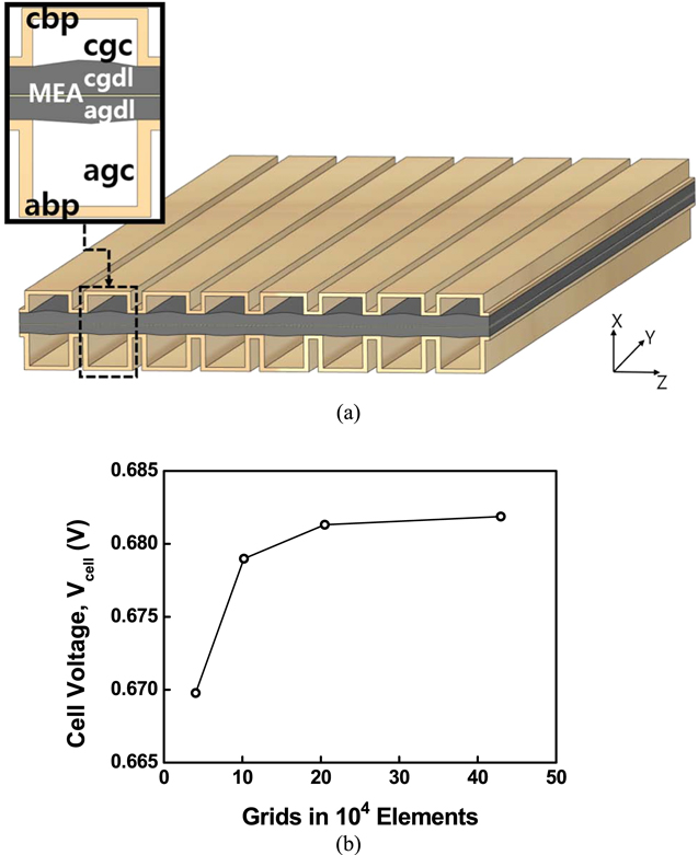
Figure 1. (a) Structure of the PEMFC (b) grid-independence test results for the 3D PEMFC model simulations.
Download figure:
Standard image High-resolution imageTable VI. Boundary conditions.
| Description | Expression | |
|---|---|---|
| Anode inlet velocity |
| (70) |
| Cathode inlet velocity |
| (71) |
| Constant temperature on side walls |

| (72) |
| Heat flux on the top and bottom surfaces |

| (73) |
| Electric potential on anode outer BP surface |

| (74) |
| Electric potential on cathode outer BP surface |
| (75) |
Metamodeling and Optimization
Metamodels or surrogates have been extensively used to mimic the functioning of expensive and time-consuming computer simulations. These surrogates assist in engineering design optimization with better performance indices than that afforded by computer simulations. Surrogate-assisted optimization usually comprises four steps: selecting the training points in the domain of interest or design space, constructing appropriate surrogate models, testing the model accuracy, and finding the global best. Figure 2 presents the surrogate-based optimization methodology.

Figure 2. Flowchart for the surrogate-based optimization technique.
Download figure:
Standard image High-resolution imageThe modeling of the surrogate necessitates the usage of sample points within the design space that is generated using the LHS technique developed by McKay et al. 32 LHS is a stratified technique wherein the range of input variables is split into Q intervals with identical and independent distribution, where Q is the number of sample points. In this study, 85 sample points are generated using LHS, it is further divided into 69 training and 16 test data. Specifically, the LHS technique that minimizes the maximum distance is used to obtain training data with an even distribution. Considering 69 training points, the surrogates (RSA, RBNN, and KRG) are constructed and then tested against 16 test points to verify the model accuracy. To verify the model prediction accuracy, root mean square error (RMSE) and adjusted R-square (adjustetd R2) are used as indicators. Both indicators convey the goodness of fit measures for the surrogate models in different ways; they will be discussed in the section of surrogate error analysis.
After checking the model's accuracy, the optimization algorithm can be applied to determine the global best. Herein, the stochastic algorithms PSO and GA are applied. After determining the optimal design points, the predicted values are compared with the CFD simulation results to validate the proposed optimization models. The detailed construction and working of the surrogates, i.e., RSA, RBNN, and KRG, are described in the metamodeling and optimization section. Further, the theory and method of optimization using PSO and GA, respectively, are briefly explained.
Response surface approximation (RSA)
RSA is an imperative technique based on mathematical and statistical methods and is used to build global approximations of an objective via functional evaluations at various points in the design space. In this study, RSA is used to denote a polynomial approximation wherein the training data are fitted by least square regression.
Generally, when a process with an observed response  input variables (
 ), and number of design input variables d are considered, the response of the process in terms of the variables is given as follows.
33
), and number of design input variables d are considered, the response of the process in terms of the variables is given as follows.
33

where  is the actual response function and
  is the source of errors that are not accounted for in
  Since the form of the actual response function is unknown, RSA is used to develop an approximate function for the actual function
  The approximation is usually performed using a polynomial function and it aims to find a predicted response within the region of interest. The polynomial that is used to represent the predicted response
  is usually a first- or second-order equation represented in Eqs. 2 and 3, respectively.
33
is usually a first- or second-order equation represented in Eqs. 2 and 3, respectively.
33

where  represent the set of input variables and the
  parameters are called the weight coefficients.
Furthermore, we demonstrate the response surface generation using a second-order function approximation. The advantage of using the second-order equation (Eq. 3) is that it can smooth out the various levels of errors in the data and can capture the global trend in the variations; this makes it more robust and well suited for engineering design optimization. Based on the training data, the weight coefficients are determined by minimizing the mean square error (MSE) between the observed data and the prediction values, which is given as

where  denotes the observed data at the set of input variables, while
  denotes the prediction values obtained using Eq. 3 within the range of N training data. To simply solve Eq 4, a matrix system is constructed (Eqs. 5 and 6).

where p represents the number of weight coefficients in each second-order equation that can be expressed in terms of the number of design variables d,  Since N training data points yield N number of responses (
 ) and errors (
 ), the dimension of
  should be
  Equation 4 is further extended and expressed in the form of a matrix system as
where L denotes the least square function. To determine the weight coefficient vector,  L is minimized by setting its derivative,
  as zero.

By simplifying Eq. 8, the expression of B is given by

Radial basis neural network (RBNN)
Neural networks are surrogate models that mimic the neuron structure. Neurons, the basic building blocks of nerves, are composed of three parts: receiving, processing, and judgement parts. As shown in Fig. 3, these are named input, hidden, and output layers, respectively. After the input layer receives information, the hidden layer processes the information, and then, the output layer makes a prediction. The function that processes information in the hidden layer is called the activation function. The activation function type varies depending on the neural network used. In the RBNN method, the Gaussian-radial function is used as the activation function, i.e., expressed as a function of input vector  comprising design variables (
 ) as follows:

where  is the
  activation function. Moreover,
  and
and  are the center and variance of input training data, respectively. ∥∥ denotes the Euclidean norm.

Figure 3. RBNN structure.
Download figure:
Standard image High-resolution imageThe output layer that is the predicted response of RBNN is a linear combination of the activation functions and the corresponding weights, and it is given as

where  denotes the predicted value for an input vector
  and
and  is the
  th weight coefficient. Further, m is the number of activation functions and weight coefficients that should be less than the number of training data points (
 ). Since the accuracy of the RBNN model depends on the
  values, the learning process of the model denotes the calculation process of the best
  values. Based on the training data in the given domain space
 is determined by minimizing the sum-squared error (
 ) between the observed data and the prediction values:

where  represents the observed response at individual
  while
while  is a prediction value shown in Eq. 11. The weight coefficients
  are estimated using the least square solution of Eq. 12 in the matrix form of
B
:
are estimated using the least square solution of Eq. 12 in the matrix form of
B
:

where  is a design matrix comprising the individual activation functions. Here, the dimension of
  should be
  where N training data points of the input layer are assigned to m activation functions of the hidden layer.
  is a
is a  vector containing observed responses corresponding to the training data points,
Kriging (KRG)
KRG 34 is a well-known surrogate model used to predict an accurate approximation in the design space. It can be used to predict both linear and nonlinear trends in the design space. The model herein is constructed using Eqs. 15–21.
The ith input vector of d-dimension is represented as 

As the observed response at  is taken as
  the vector for all N observed responses is

Suppose that the predicted response from the KRG model at  is
is  then the distance between any two chosen design points
  and
and  is correlated with the prediction values. i.e., the difference between the predicted values reduces with the interval between the two points. The relationship between the correlated values is

where  and
and  represent the
  th components of
  and
and  respectively, and
  is their regression parameter. The correlation values at all the observed points can be written in terms of a
  matrix
  i.e.,
i.e.,
The KRG predictor  is
is

where  is a singular matrix of size
  and
and  is the mean value of the training dataset distribution that is calculated through maximum likelihood estimation:

Here,  is the vector comprising correlation values between a given prediction point and all training data. The structure of
  is expressed as

Particle swarm optimization (PSO)
PSO is one of the most widely used optimization technique developed by Kennedy and Eberhart,
35
and it is based on the communal behavior of particles in a population, and is also known as a swarm. The algorithm is a metaheuristic that is used to optimize nonlinear continuous functions and is based on an evolutionary search to obtain the global best. Figure 4 describes the functioning of the algorithm. In PSO,
S
represents the population of N number of particles, and the particles represent points that are uniformly distributed within the dimensional space  where each particle can flow through
  based on their individual and swarm behaviors.

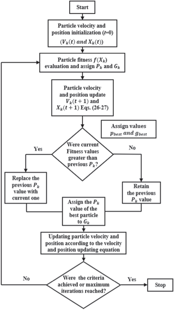
Figure 4. Flowchart of the PSO algorithm.
Download figure:
Standard image High-resolution imageAccordingly, the position, velocity, and fitness values of the  th particles (
 ) can be described in the form of a vector, as given in Eqs. 23–25
Position vector,

Velocity vector,

Fitness values,

In Eq. 25,  is the objective function at each
  While searching for the optimal solution for the given problem, the particles update their positions and velocities according to each iteration as follows:
Particle velocity update,

Particle position update,

where  and
and  indicate two consecutive iterations of the algorithm.
  and
and  are the velocity and position vectors of the particle k at the
  iteration, respectively. Further,
  denotes the "personal best" of the
  particle, i.e., the position of the best solution obtained during the entire iteration.
  denotes the "global best," representing the position of the overall best solution obtained in the population group (S).
 are the acceleration factors and
  and
and  are random numbers between 0 and 1. As shown in Eq. 26,
  is depends on three terms: the inertia term,
  cognitive term,
  and social term,
  While the inertia term prevents the particle from making drastic changes in direction by keeping a trail of the previous flow direction, the cognitive term helps the particle return to its previous best solution and the social term directs the particles to move toward the best solution in the entire population. While updating
  the acceleration factors
  which modulate the magnitudes of the steps in the direction of its personal best and global best, respectively, are usually chosen within the range of 0–4.
36
which modulate the magnitudes of the steps in the direction of its personal best and global best, respectively, are usually chosen within the range of 0–4.
36
Figure 4 briefly shows the working procedures of the PSO algorithm that comprises the following basics steps:
- 1.Initialization step.
- 2.Iteration step.
- 3.Judging the best solution.
In the initialization step, the size of
S
is defined (k = 1, 2, ..., N) and the initial positions of the particles are considered as  At every
 is initialized to
  The fitness values of all particles at
  are evaluated as
  and the particle with the highest fitness value is assigned as the global best,
  In the second step, the values of
  and
and  are updated to
  and
and  according to Eqs. 26 and 27, respectively, and the fitness values
  are evaluated. If the updated fitness values
  are greater than the previous fitness values
  the
the  values are assigned to new
  (
( ). Similarly, the global best
  is updated by evaluating whether
  is greater than the desired fitness
  The algorithm terminates after all the particles reach the same global best value
  or the maximum iteration has been reached.
Genetic algorithm
Similar to PSO, GA employs metaheuristic and iterative processes for optimization inspired by natural selection. The optimization process mimics biological processes wherein genes are selected, mated, and mutated. 37 GA comprises the following four steps (Fig. 5): generation of parent chromosomes, mating, selection, and mutation.
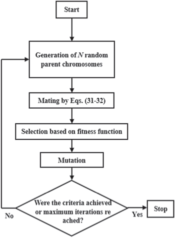
Figure 5. Flowchart of the GA.
Download figure:
Standard image High-resolution imageIn the first step, the process begins by randomly generating 1st generation parent chromosomes to form population P, comprising N number of design vectors called chromosomes, which is denoted by  (
( ). Each chromosome is a d-dimensional vector comprising d number of genes represented by
  random values between 0 and 1 are assigned to it.
  and
and  are expressed as follows:


In GA, the individual chromosomes in population P are evaluated at the end of each generation, where the fitness value (i.e., objective function value  ) is represented as

Once the  generation of N chromosomes have been released, the second step, i.e., mating, begins to produce new offsprings N. Two offsprings
 ![${{\boldsymbol{X}}}_{w}=\left[{x}_{w1},{x}_{w2},\cdots ,{x}_{wd}\right]$](https://content.cld.iop.org/journals/1945-7111/169/1/014511/revision2/jesac492fieqn216.gif) and
and ![${{\boldsymbol{X}}}_{z}=\left[{x}_{z1},{x}_{z2},\cdots ,{x}_{zd}\right]$](https://content.cld.iop.org/journals/1945-7111/169/1/014511/revision2/jesac492fieqn217.gif) are afforded from two random parents in P, namely,
are afforded from two random parents in P, namely, ![${{\boldsymbol{X}}}_{f}=\left[{x}_{f1},{x}_{f2},\cdots ,{x}_{fd}\right]$](https://content.cld.iop.org/journals/1945-7111/169/1/014511/revision2/jesac492fieqn218.gif) and
and ![${{\boldsymbol{X}}}_{m}=\left[{x}_{m1},{x}_{m2},\cdots ,{x}_{md}\right].$](https://content.cld.iop.org/journals/1945-7111/169/1/014511/revision2/jesac492fieqn219.gif) The process of generating offsprings is controlled by the mating rate q that varies between 0 and 1:
The process of generating offsprings is controlled by the mating rate q that varies between 0 and 1:
Offspring 1,

Offspring 2,

where  and
and  represent the
  genes (
 ) of the offsprings 1 and 2, respectively. At the end of the mating process, a total population of 2N is obtained.
In the third step, based on the fitness values of individual chromosomes, N chromosomes with high fitness values are selected among 2N chromosomes. In the final step, a mutation that induces changes in genes of random chromosomes is performed with a very small predetermined probability of 0.1 to secure genetic diversity. 38 Then, the newly selected N chromosomes become parent chromosomes in the next iteration. Thereafter, the iterative process continues from step 2 until the stopping criteria are met, i.e., a satisfactory fitness level has been obtained for the population or a maximum number of allowed iterations has been reached.
Surrogate error analysis
Once the surrogate models are developed using the generated training data, the accuracy of these models is tested at 16 test points, i.e. selected from 85 sample points. Numerical error estimators ( and RMSE) are used to evaluate the accuracy of the surrogate models, i.e., using Eqs. 33 and 34, respectively.

where r is the number of test data points. Moreover,  and
and  denote the observed responses that can be obtained using CFD simulations and the predicted values from the surrogate models, respectively;
  denotes the mean value of the observed data at r test points and
  is the number of design parameters. The obtained
  and RMSE values demonstrate the fit of the model with the data considered herein. The
  values range from zero to one, where zero indicates a poor model accuracy and a value close to one indicates perfect predictions. For RMSE, smaller values, i.e., close to zero, indicate better model accuracy and higher values, i.e., close to one, indicate poor accuracy.
Result and Discussion
As a measure of the optimum cell performance, this study considers the maximum voltage (V) generated within the cell as the design objective. Figure 6a shows the schematic of a PEMFC single-cell geometry with a straight channel flow field. The GDL thickness (δgdl ), channel depth (dch ), channel width (wch ), and land width (wland ) are considered as the design variables; they range from 0.05 to 0.4 mm for δgdl , 0.3 to 2.0 mm for dch , 0.3 to 2.0 mm for wch , and 0.3 to 1.0 mm for wland . Subsequently, the optimization problem can be formulated as follows:

where the units are in mm
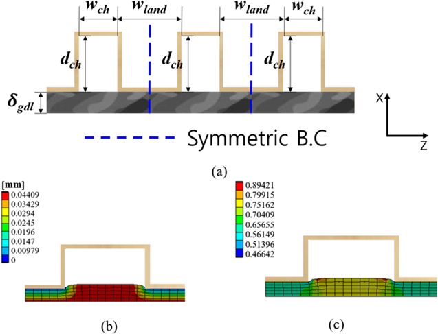
Figure 6. (a) Schematic of the fuel cell structure along with the design variables. (b) Deformation (mm) along the x-direction in the cathode GDL. (c) Porosity distribution in the cathode GDL.
Download figure:
Standard image High-resolution imageAdditionally, for more realistic fuel cell simulations, the compression/intrusion of GDL during cell assembly process is considered using the FSI technique and its influence on the local transport behavior and overall cell performance is analyzed. In this study, a typical GDL widely used for fuel cell applications, i.e. SGL® 10BA was chosen and its mechanical properties are listed in Table III. The GDL shapes before and after cell assembly are displayed in Fig. 6, where GDL is deformed by the channel-land structure of the flow field, implying that the GDL porosity varies depending on the dimensions of the flowfield (

 ) and GDL (
 ) as well as the compression ratio. Figures 6b and 6c show the deformation and porosity distributions of the cathode GDL for the reference cell design (
 and
and  ) under 20% GDL compression (the thickness of GDL is reduced by 20% from its initial value), respectively. As seen in Fig. 6b, the GDL deformation underneath the lands is more evident than the area under the channel. Subsequently, Fig. 6c shows that the GDL porosity near the lands ranges from 0.6 to 0.65, while the porosity under the channel is relatively uniformly maintained at the initial GDL porosity level before cell assembly (i.e., 0.65–0.89). Based on the above discussion, the reference cell design is simulated for operating current densities from 0.1 to 2.0 A cm−2, which is compared with the optimized designs in Fig. 14.
To commence the optimization process, 85 design points are generated through the LHS technique between the upper and lower bounds of each design variable. These points constitute 69 design points employed for the training set and 16 design points employed for the test set. The distributions of the training and test set points are provided in Figs. 7a and 7b, respectively. The training data points evenly cover the entire design space. The cell voltages predicted by the PEMFC model are summarized in Table VII for the training set and Table VIII for the test set. After the surrogate models are constructed using the training set, their accuracies are evaluated over the training and test sets using the two-performance metrics: RMSE and adjusted  Moreover, the consideration of the training accuracy provides a way for selecting the best performing algorithm and for fine tuning the model parameters. Figure 8 shows the scatter plots for the training set; they depict the correlation between the values obtained through the 3D PEMFC simulations and values predicted through the three different surrogate models employed herein. The figure shows that the three models accurately represent the system, where the RMSE values for RSA, RBNN, and KRG are 4.98, 0.26, and 0 mV. Moreover, the adjusted
  values for RSA, RBNN, and KRG are 0.8945, 0.999, and 1.000, respectively. These values are sufficient for implying no overfitting problems in the constructed surrogate. RBNN and KRG can afford high adjusted
  values regardless of the data since the surrogate models well fit the nonlinear data. However, in RSA, the adjusted
  value for the training dataset tends to vary with the number of training data. Herein, the adjusted
  value for RSA of approximately 0.9 was desired, and it is achieved by considering 69 training data sets. To check the effectiveness of the trained models, 16 test points, i.e., drawn from the parameter space (Fig. 7b), are applied to the three surrogate models; their accuracies are compared in Fig. 9. The RMSE values for RSA, RBNN, KRG model are 4.33, 3.33, and 2.53 mV, while the adjusted
  values for these models are 0.8402, 0.9054, and 0.9455 respectively. A comparison of these errors clearly indicates that the KRG model outperforms the RBNN and RSA models in terms of predicting the cell voltage at the 16 test points. This is due to the differences in the features among the surrogate models. The RSA model is based on global approximation, whereas the KRG and RBNN models are based on local approximation. Particularly, the RSA model uses a global approximation based on quadratic polynomial equation; it can cause overprediction problems in engineering with nonlinear and multimodal characteristics. In contrast, by adopting local approximation through the interpolation method, a fitness function can be generated in the KRG and RBNN models by considering many inflection points. Thus, surrogate models with low relative errors can be constructed. Based on the error comparison analysis, the KRG and RBNN models, which can represent many inflection points, can afford a relatively accurate fitness function in fuel cell engineering with nonlinear features, such as the present optimization problem.
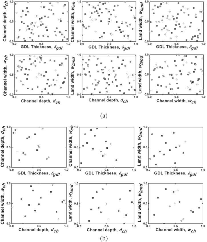
Figure 7. LHS distributions for (a) the training data of 69 operating points and (b) the test data of 16 operating points.
Download figure:
Standard image High-resolution imageTable VII. Training data set and 3D PEMFC model predictions I = 1.5 A cm−2.
| Cases | GDL thickness,  [mm] [mm] | Channel depth,  [mm] [mm] | Channel width,  [mm] [mm] | Land width,  [mm] [mm] | Cell voltage, Vcell (3D PEMFC simulation) [mV] |
|---|---|---|---|---|---|
| 1 | 0.0569 | 1.9 | 1 | 0.643 | 677.16 |
| 2 | 0.105 | 1.6 | 1.333 | 0.904 | 667.04 |
| 3 | 0.16 | 0.667 | 1.4 | 0.973 | 681.27 |
| 4 | 0.208 | 0.533 | 1.7 | 0.698 | 696.71 |
| 5 | 0.304 | 1.467 | 0.7 | 0.767 | 668.17 |
| 6 | 0.311 | 0.3 | 1.067 | 0.3 | 706.21 |
| 7 | 0.05 | 0.733 | 0.567 | 0.465 | 696.98 |
| 8 | 0.174 | 0.633 | 1.167 | 0.492 | 703.41 |
| 9 | 0.352 | 1.167 | 0.433 | 0.725 | 637.02 |
| 10 | 0.386 | 0.767 | 1.367 | 0.822 | 689.85 |
| 11 | 0.119 | 0.333 | 0.3 | 0.918 | 636.68 |
| 12 | 0.201 | 0.933 | 1.933 | 0.739 | 689.43 |
| 13 | 0.153 | 0.467 | 1.5 | 0.424 | 702.92 |
| 14 | 0.194 | 1.4 | 0.667 | 0.451 | 696.49 |
| 15 | 0.318 | 0.567 | 0.733 | 0.63 | 697.45 |
| 16 | 0.167 | 0.367 | 0.467 | 0.753 | 690.07 |
| 17 | 0.235 | 1.033 | 0.633 | 0.78 | 678.8 |
| 18 | 0.379 | 1.867 | 0.833 | 0.437 | 684.77 |
| 19 | 0.0775 | 0.5 | 0.867 | 0.794 | 681.04 |
| 20 | 0.125 | 1.433 | 1.767 | 0.959 | 666.78 |
| 21 | 0.27 | 1.333 | 0.767 | 0.616 | 688.59 |
| 22 | 0.338 | 1.233 | 1.1 | 0.89 | 675.51 |
| 23 | 0.366 | 1.5 | 0.333 | 0.369 | 680.02 |
| 24 | 0.359 | 0.6 | 1.8 | 0.314 | 697.05 |
| 25 | 0.187 | 1.1 | 1.9 | 0.355 | 692.62 |
| 26 | 0.222 | 1 | 1.033 | 0.588 | 697.54 |
| 27 | 0.228 | 1.3 | 1.267 | 0.712 | 689.71 |
| 28 | 0.0843 | 0.8 | 1.967 | 0.931 | 662.85 |
| 29 | 0.112 | 1.067 | 1.2 | 0.41 | 700.77 |
| 30 | 0.18 | 0.967 | 1.533 | 0.684 | 693.69 |
| 31 | 0.325 | 0.867 | 0.533 | 0.341 | 699.81 |
| 32 | 0.37 | 1.8 | 1.633 | 0.506 | 686.43 |
| 33 | 0.0706 | 0.433 | 1.467 | 0.863 | 674.31 |
| 34 | 0.215 | 1.267 | 1.667 | 0.52 | 693.81 |
| 35 | 0.283 | 1.933 | 1.833 | 0.547 | 684.19 |
| 36 | 0.132 | 1.733 | 1.567 | 0.671 | 683.82 |
| 37 | 0.256 | 0.9 | 1.633 | 0.849 | 688.68 |
| 38 | 0.297 | 1.833 | 0.8 | 0.877 | 629.57 |
| 39 | 0.249 | 1.367 | 0.367 | 0.561 | 674.26 |
| 40 | 0.331 | 1.967 | 2 | 0.382 | 681.38 |
| 41 | 0.0637 | 1.533 | 0.933 | 0.478 | 692.67 |
| 42 | 0.098 | 1.133 | 1.867 | 0.575 | 686.53 |
| 43 | 0.276 | 1.667 | 1.133 | 0.808 | 675.72 |
| 44 | 0.4 | 1.567 | 1.733 | 0.835 | 676.92 |
| 45 | 0.139 | 2 | 1.233 | 1 | 651.56 |
| 46 | 0.146 | 0.833 | 1.6 | 0.533 | 697.47 |
| 47 | 0.242 | 1.767 | 0.6 | 0.602 | 676.41 |
| 48 | 0.291 | 1.633 | 0.9 | 0.327 | 694.67 |
| 49 | 0.345 | 0.7 | 0.967 | 0.396 | 701.40 |
| 50 | 0.393 | 0.4 | 1.3 | 0.657 | 698.73 |
| 51 | 0.138 | 1.578 | 0.725 | 0.3 | 699.95 |
| 52 | 0.05 | 1.15 | 1.788 | 0.475 | 681.96 |
| 53 | 0.313 | 0.725 | 1.15 | 0.563 | 699.62 |
| 54 | 0.225 | 1.788 | 1.575 | 0.388 | 690.67 |
| 55 | 0.225 | 1.15 | 1.15 | 0.65 | 694.36 |
| 56 | 0.181 | 0.3 | 0.513 | 0.825 | 688.33 |
| 57 | 0.0938 | 1.363 | 0.938 | 0.65 | 685.8 |
| 58 | 0.269 | 0.513 | 1.363 | 0.913 | 691.23 |
| 59 | 0.375 | 0.482 | 1.757 | 0.825 | 693.13 |
| 60 | 0.238 | 0.543 | 1.454 | 0.675 | 686.66 |
| 61 | 0.363 | 0.361 | 1.023 | 0.4 | 703.76 |
| 62 | 0.263 | 0.786 | 1.818 | 0.475 | 696.93 |
| 63 | 0.113 | 0.421 | 1.514 | 0.65 | 694.64 |
| 64 | 0.35 | 1.271 | 0.543 | 0.775 | 648.67 |
| 65 | 0.2495 | 0.385 | 0.385 | 0.629 | 702.85 |
| 66 | 0.302 | 0.428 | 0.909 | 0.388 | 705.11 |
| 67 | 0.33 | 0.47 | 0.81 | 0.3 | 705.69 |
| 68 | 0.33 | 0.3 | 0.98 | 0.58 | 703 |
| 69 | 0.225 | 0.3 | 1.15 | 0.3 | 707.1 |
Table VIII. Test data set and 3D PEMFC model predictions I = 1.5 A cm−2.
| Cases | GDL thickness,  [mm] [mm] | Channel depth,  [mm] [mm] | Channel width,  [mm] [mm] | Land width,  [mm] [mm] | Cell voltage, Vcell (3D PEMFC simulation) [mV] |
|---|---|---|---|---|---|
| 1 | 0.15 | 1.524 | 1.636 | 0.525 | 691.1 |
| 2 | 0.213 | 1.029 | 0.846 | 0.9 | 674 |
| 3 | 0.25 | 1.939 | 1.271 | 0.675 | 682.3 |
| 4 | 0.275 | 0.664 | 0.3 | 0.55 | 689.63 |
| 5 | 0.138 | 0.846 | 1.089 | 0.85 | 683.71 |
| 6 | 0.1 | 0.604 | 1.332 | 0.35 | 700.79 |
| 7 | 0.228 | 1.15 | 1.12 | 0.65 | 693.99 |
| 8 | 0.163 | 1.575 | 1.939 | 0.725 | 680.96 |
| 9 | 0.088 | 0.968 | 1.696 | 0.5 | 691.9 |
| 10 | 0.188 | 0.3 | 0.968 | 0.6 | 704.2 |
| 11 | 0.222 | 1.211 | 1.393 | 0.375 | 698.18 |
| 12 | 0.075 | 1.879 | 1.211 | 0.875 | 656.33 |
| 13 | 0.2 | 1.696 | 0.786 | 0.3 | 697.61 |
| 14 | 0.288 | 0.725 | 0.604 | 0.75 | 687.12 |
| 15 | 0.063 | 1.757 | 0.482 | 0.45 | 684.45 |
| 16 | 0.125 | 0.907 | 1.879 | 0.575 | 690.13 |
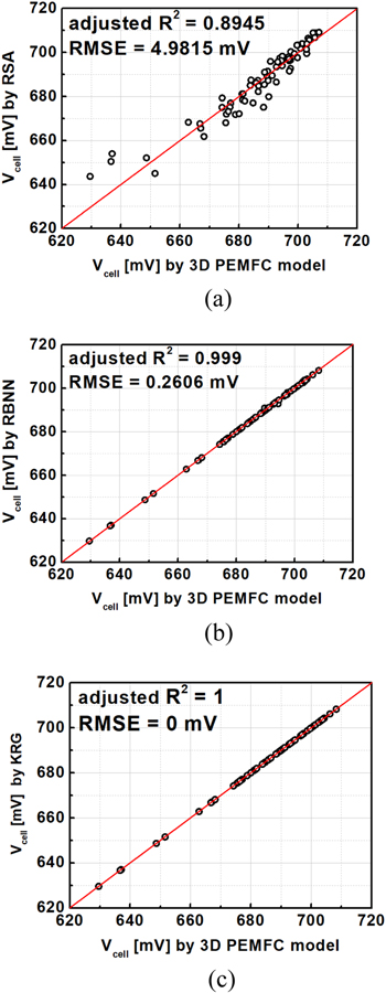
Figure 8. Scatter plots for the training set that depict the correlation between the cell voltages simulated by the 3D PEMFC model and cell voltages predicted by the surrogate models of (a) RSA, (b) RBNN, and (c) KRG.
Download figure:
Standard image High-resolution image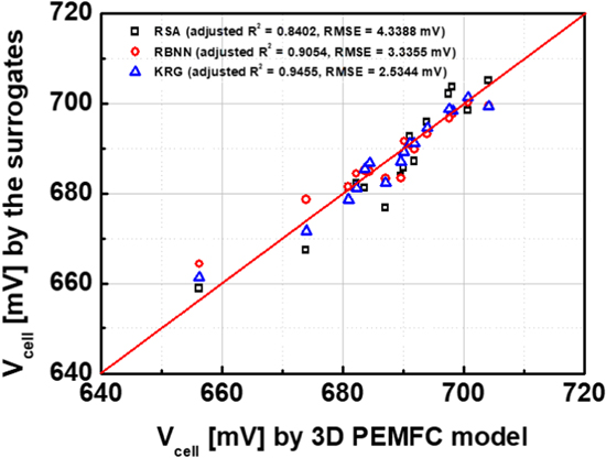
Figure 9. Scatter plot for the test set depicting the correlation between the cell voltages simulated by the 3D PEMFC model and cell voltages predicted by the surrogate models of RSA, RBNN, and KRG.
Download figure:
Standard image High-resolution imageSubsequently, these models are integrated with the two optimization algorithms (PSO and GA) to obtain optimum values for the four design variables. By virtue, the optimization algorithms begin by generating a random initial population in the defined search space, wherein the random initial population and the number of iterations are set to 200 and 1000, respectively. Since randomness in the optimal result is obtained in every run of the optimization algorithm, the algorithms are run until a constant optimal value is obtained. Table IX summarizes the optimum values of the four design variables and the corresponding cell voltages predicted by the individual surrogate and reference models. The optimum values of the design variables obtained using PSO and GA and the corresponding cell voltages predicted by the three surrogate models are similar to each other. Furthermore, when the optimum design values are applied to the PEMFC model and simulated, all the PEMFC simulation results are at the 0.708 V level. Therefore, subsequent analysis and discussion are based on the optimal values obtained using the PSO search algorithm. Compared to the PEMFC simulation results, the performance deviations for RSA, RBNN, KRG surrogates at I = 1.5 A cm−2 are 0.77, 1.26, 0.24 mV, respectively, demonstrating that these surrogate models afford sufficient accuracy for optimizing key PEMFC design variables.
Table IX. Optimum values of design variables predicted by the surrogate models.
| Surrogate model/Optimization algorithm | |||||||
|---|---|---|---|---|---|---|---|
| RSA | RBNN | KRG | |||||
| Description | PSO | GA | PSO | GA | PSO | GA | Reference condition |
GDL thickness  [mm] [mm] | 0.215 | 0.212 | 0.207 | 0.201 | 0.221 | 0.215 | 0.215 |
Channel depth,  [mm] [mm] | 0.300 | 0.309 | 0.614 | 0.640 | 0.410 | 0.434 | 0.54 |
Channel width,  [mm] [mm] | 0.975 | 0.988 | 0.825 | 0.821 | 0.790 | 0.766 | 1 |
Land width,  [mm] [mm] | 0.300 | 0.328 | 0.396 | 0.412 | 0.300 | 0.309 | 1 |
| Surrogate model predictions [mV] at I = 1.5 A cm−2 | 709 | 708.8 | 710 | 710 | 708.3 | 708.3 | — |
| PEMFC simulation results [mV] at I = 1.5 A cm−2 | 708.23 | 708.4 | 708.74 | 708.3 | 708.06 | 708.1 | 681 |
To understand the detailed influence of each design variable on the cell performance, model predictions by the RSA, RBNN, and KRG methods are plotted in Figs. 10–12, respectively. These plots are drawn for each design variable against the cell voltage by placing the other three constant variables at their optimal values. For example, in Fig. 10a, the effect of varying GDL thickness ( ) on cell voltage is observed by placing the other design variables at their optimal values (
 and
and  ). As shown in Figs. 10a–12a, the observation of the variation effects of
  reveals that a thinner GDL are disadvantageous in terms of oxygen and electron transport along the in-plane (z) direction (it is expected that the oxygen transport is usually more hampered than the electron transport) whereas a thicker GDL limits the oxygen transport along the through-plane (x) direction. Due to the opposing effects, the optimum values of GDL thickness predicted by the RSA, RBNN, and KRG models are between its upper and lower bounds (
 ) and predicted to be 0.215, 0.207, and 0.221 mm, respectively. Regarding the influence of channel depth (
 ), a tradeoff exists between the oxygen transport/water removal capability and the ability to tolerate GDL intrusion. Since the same cathode stoichiometry of 2.0 is applied to all simulation cases, the larger
  corresponds to the lower overall air velocity in the gas channel; this weakens the oxygen transport and the removal of water that is accumulated inside the cathode GDL. In contrast, a reduced
  is more susceptible to the GDL intrusion, which can decrease the cell performance if the GDL intrusion level becomes prominent and consequently severe flow maldistribution of the reactant gases occurs over the cell.
39–41
Figures 10b–12b show that the cell voltage generally decreases with increasing
is more susceptible to the GDL intrusion, which can decrease the cell performance if the GDL intrusion level becomes prominent and consequently severe flow maldistribution of the reactant gases occurs over the cell.
39–41
Figures 10b–12b show that the cell voltage generally decreases with increasing  This is clearly indicative of the dominant effect of the convective airflow and the resulting GDL flooding while the extent of flow maldistribution is minimal. The optimum
  value for RSA is exactly the lower bound value (0.3 mm), while those for RBNN and KRG are 0.614 and 0.41 mm. Note that a smaller
  induces a higher pressure drop, consequently demanding a larger pumping power for the reactant supply, which should also be considered in actual cell and stack designs. The
  and
and  dimensions are mainly related to the lateral transport of electrons and oxygen. A wider
  facilitates the lateral oxygen diffusion from the channel to land regions but limits the lateral electron transport from the cathode CL region underneath the channel to the current collecting lands, and vice versa for
  It is particularly evident that a larger
  design should be avoided since the GDL region underneath the lands is compressed and is thus vulnerable to oxygen transport and flooding.

Figure 10. Effects of (a) GDL thickness,  (b) channel depth,
  (c) channel width,
  and (d) land width,
  on the cell voltage, Vcell, predicted by RSA.
Download figure:
Standard image High-resolution image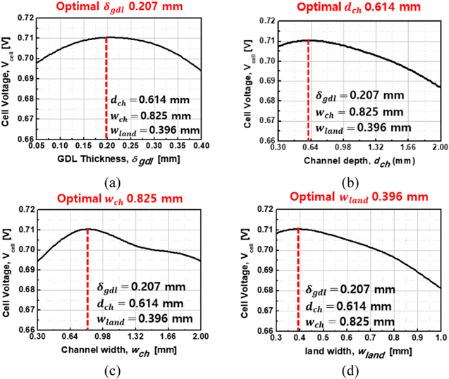
Figure 11. Effects of (a) GDL thickness,  (b) channel depth,
  (c) channel width,
  and (d) land width,
  on the cell voltage, Vcell, predicted by RBNN.
Download figure:
Standard image High-resolution image
Figure 12. Effects of (a) GDL thickness,  (b) channel depth,
  (c) channel width,
  and (d) land width,
  on the cell voltage, Vcell, predicted by KRG.
Download figure:
Standard image High-resolution imageDue to strong cell voltage interactions with  and
and  the cell voltage is plotted as a function of
  and
and  in Fig. 13. The figure shows a noticeable drop in the voltage performance at the extreme channel and land dimension values. When
  is at the lower side and
  is at the higher side, minimum cell performance around Vcell = 0.63 V is observed for all the three surrogates, clearly indicating the dominant effect of oxygen transport within the cell. The larger values of
  and
and  also lower the cell performance due to the oxygen and electron transport difficulties. The narrow
  design is well compatible with a wide range of
  (from 0.3 to 2.0 mm). The maximum cell performance is predicted with
  = 0.975/0.3 mm for RSA, 0.825/0.396 mm for RBNN, and 0.79/0.3 mm for KRG. The
  interaction contours in Fig. 13 indicate that the
  values from 2 to 3.25 afford optimal PEMFC performances, providing a good insight on a suitable flowfield design strategy to ensure effective oxygen and electron transport.

Figure 13. Contour plots for cell performance considering interactions of  and
and  using the three surrogate models: (a) RSA at
  = 0.215
  and
and  (b) RBNN at
  = 0.207
  and
and  and (c) KRG at
  =
=  and
and 
Download figure:
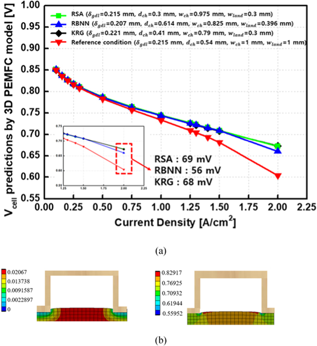
Standard image High-resolution imageFinally, 3D PEMFC model simulations are conducted using the optimum values of the four design variables predicted by the three surrogate models (Table IX). Based on the simulation results, the polarization curves are drawn for current densities from 0.1 to 2.0  in Fig. 14a. The cell performance with the optimum design conditions obtained by the surrogate models is significantly better than that with the reference design. At 2.0
  the performance improvement is around 69 mV for RSA, 56 mV for RBNN, and 68 mV for KRG. Particularly,
  = 1:1 in the reference condition causes a significant cell performance drop in the high current density region due to more restrictive oxygen transport. The deformation and porosity distributions for the optimum design condition predicted by KRG are plotted in Fig. 14b. The lower deformation and porosity variations are observed compared to those of the reference design (Figs. 6b and 6c), which is due mainly to the narrower land width (
 = 0.3 mm) and the larger channel to land ratio (
 = 2.63) for the KRG design. Interestingly, note that similar cell performances are obtained by the optimum design conditions predicted by RSA, RBNN, and KRG, despite the different optimum values (Table IX).
Figure 14. (a) Comparison of the polarization curves obtained by 3D PEMFC model simulations. The optimum values of the four design variables predicted by the RSA, RBNN, and KRG surrogates are given in Table IX along with the reference condition. (b) Deformation (mm) distribution along the x-direction (Left) and porosity distribution (Right) in the cathode GDL for the optimal case predicted by KRG.
Download figure:
Standard image High-resolution image
Conclusions
This study employed three famous surrogate models, i.e., KRG, RBNN, and RSA, with stochastic optimization algorithms, i.e., PSO and GA, to search for the global optimum values of key PEMFC design variables: GDL thickness ( channel depth (
 ), channel width (
 ), and land width (
 ). First, the surrogates were constructed and tested using the simulation results of a multiscale, two-phase, 3D PEMFC model wherein a special emphasis was placed on considering the effects of GDL compression/intrusion via FSI simulations. Then, the performance prediction capabilities of the surrogate models were compared. According to adjusted R2 and RMSE analyses using the test set of 16 design points, the KRG model outperformed the RBNN and RSA models; the accuracy of the RSA model was relatively poor. After the surrogates were integrated into the PSO or GA optimization algorithms, the optimal design values were successfully obtained. The performance deviations between the RSA, RBNN, and KRG predictions and the PEMFC model simulation results at I = 1.5 A cm−2 were 0.77, 1.26, 0.24 mV, respectively. Finally, polarization curves were drawn through the PEMFC model simulations at the optimal points obtained from the three surrogates, and comparison with the reference design demonstrated that the cell voltage was improved by around 56–69 mV at 2.0
  Thus, this study successfully demonstrated the potential of using surrogates and optimization algorithms to alleviate the burden of expensive and time-consuming optimization procedures of PEMFC design and operating conditions.
Acknowledgments
This study was supported by Korea Institute of Energy Technology Evaluation and Planning (KETEP), Ministry of Trade, Industry and Energy (MOTIE), Republic of Korea (No. 20188550000440) as well as by the the Technology Innovation Program of the Korea Evaluation Institute of Industrial Technology (KEIT) under the MOTIE of Republic of Korea (No. 20012121) We would also like to thank TAESUNG S&E, Inc., Seoul, Republic of Korea, for providing technical support for ANSYS Fluent software.