
Abstract
Atomic emission spectroelectrochemistry (AESEC) combined with linear sweep voltammetry (LSV) and electrochemical impedance spectroscopy (EIS) provided insights on both active and passive dissolution of Ni-Fe-Cr-Mn-Co multi-principal element alloy. Elemental dissolution rates measured by AESEC during open circuit experiment were in agreement with those extrapolated from AESEC-LSV and indicated element-specific dissolution tendencies. AESEC-EIS at open circuit potential showed nearly in-phase elemental dissolution during potential modulation which suggests direct dissolution from the alloy surface to the electrolyte. In the passive potential domain, no oscillation of the elemental dissolution rate was detected by AESEC-EIS, suggesting non-oxidative chemical dissolution of the outer layer of the passive film. In this case, dissolution at the passive film/electrolyte interface was equal to the metal oxidation rate (passive current density) at the metal/passive film interface and the passive current density was independent of potential.
Export citation and abstract BibTeX RIS
The interest in multi-principal element alloys (MPEAs) has increased greatly in recent years 1 due to their excellent corrosion resistance in both aqueous and non-aqueous environments, 2,3–8 enhanced resistance to thermal/radiative damages, 9–12 as well as outstanding mechanical properties. 13–15 The research on MPEAs has so far mainly focused on alloy design favoring single-phase formation and their mechanical properties, whereas the kinetic information during the corrosion of these alloys is still limited to date. A better understanding of the passivation/dissolution mechanism is required because passive films formed on MPEA can regulate the overall corrosion process as reported for metals and conventional alloy systems. 16 Unlike conventional alloys, there are several routes to explain the possible superior passivity of the MPEAs. Some of the passive film formed on the MPEA surface have been reported to be similar to conventional alloys whilst others are relatively novel. 3,6,8 For instance, if a single dominate passivating element and one minor passivating element are utilized in an MPEA, then potentially any of the following passive films could form. A complex stoichiometric oxide or a spinel involving more than one element could form. A group of phase separated oxides could form, or an equilibrium or non-equilibrium solid solution could form on a host oxide lattice. 17,18 All of these conditions may be possible under various metastable and stable conditions given the large multidimensional compositional space available, and the number of possible pathways for passivation.
Corrosion of elements in MPEAs is likely selective under certain conditions and depends on the specific chemical and electrochemical properties of each alloying element as well as their interactions with each other. Alloys with four to five elements in equiatomic portions may possess 20 to 25 at% of a single principal passivating element, which generally places them above a critical threshold to form a protective passive film consisting of one dominant element. 6,19,20 By similar reasoning, the concentrations of elements detrimental towards passivation can be minimized, however, this is not without its bounds. For instance, Mn is desired to stabilize face-centered cubic (FCC) solid solution even though it forms a film detrimental to the protection by passivity. 12,21 Early reports of passivation and oxidation assume the presence of single-element or complex oxides 22 and stoichiometric oxides. 7 In the case of aqueous passivation, surface-sensitive tools must be used because the oxides have a thickness of the order of several nanometers. X-ray photoelectron spectroscopy (XPS) probes core level photoelectrons and does not reveal long-range structure, only providing binding energies that suggest certain molecular compounds. These binding energies may be similar in the case of several molecular compounds. 23 An unresolved issue is how selective dissolution at active surfaces or multi-element oxide/electrolyte interfaces contributes to surface modification and selected oxide formation. All of these questions suggest the need for a more detailed understanding of the fate of each element during active dissolution and passivation of an alloy.
Conventional electrochemical analysis, such as electrochemical impedance spectroscopy (EIS), has been conducted to monitor operando dissolution/passivation kinetics of the MPEAs upon exposure to open circuit or constant applied potential. 24–26 The main constraint of using EIS for multi-element alloys is the uncertainty of identifying element-specific faradaic reactions participating in charge-transfer reactions. Each alloying element may contribute to the electrochemical response, especially in the case of polarization experiments such as linear sweep voltammetry (LSV), which is often significantly anodic with respect to the equilibrium oxidation potential of each element. To this end, coupling of the EIS with other analytical techniques furnishes the opportunity for a better understanding of the fate of elements at the metal/electrolyte, metal/passive film and passive film/electrolyte interfaces that might lead to oxide enrichment, ejection into solution or left behind and accumulated in the metal at the alloy/oxide interface. 27–30
Atomic emission spectroelectrochemistry (AESEC) has demonstrated to be a powerful technique to track the fate of each alloying elements for MPEAs during electrochemical measurements. 21,31–35 The fate of each element, whether in metal, oxide or solution during spontaneous dissolution, activation and passivation, was ascertained by the AESEC technique. AESEC enables the determination of atoms which are oxidized but not dissolve in solution, i.e., may have reached the surface as an oxidized insoluble species, via AESEC mass-charge balance. During corrosion, the net electrical current is composed of corrosion product formation, oxidative dissolution from the corrosion product or metallic substrate, as well as direct oxidation to form a soluble product. 36,37 These can be confounded further by a non-negligible cathodic reaction at the same time, often related to the H2 gas evolution especially in the active potential domain. 38,39 Supplementary information is often required to identify the exact stoichiometry of the reaction when using only an AESEC measurement approach.
Coupling AESEC and EIS has demonstrated to give a "better informed" view of anodic and cathodic elemental dissolution kinetics. Previously, the AESEC-EIS methodology was applied to investigate the elemental dissolution kinetics of relatively simple systems such as pure Zn in NH4Cl, 40 pure Mg 41 in NaCl, and a binary Al-32 wt% Zn single-phase alloy in NaOH. 42
In this work, we extend the AESEC-EIS analysis to a five-principal elements Ni38Fe20Cr22Mn10Co10 (at%) MPEA exposed in a 2 M H2SO4 solution in order to not only track the fate of each element but to elucidate the kinetics of elemental dissolution in both the active and passive potential domains. Elementally resolved electrochemical parameters such as elemental dissolution (corrosion) current densities, and Tafel slopes of individual elements were determined by AESEC-EIS and compared with elemental data obtained from AESEC during LSV. An Evans diagram was constructed using a combination of AESEC-LSV data while taking into account cathodic reaction rates from Tafel extrapolation of the applied current density. Both dissolution at open circuit potential (E oc ) in the active potential domain and at an applied potential in the passive domain were interrogated by AESEC-EIS analysis using specifically the decomposed elemental impedance contribution in real part (Z r (j M )). Direct dissolution from the alloy substrate during open circuit dissolution is indicated by the nearly in-phase oscillation of the dissolution rate signals of all alloying elements in response to AC voltage excitation. When steady dissolution occurred on the passivated surface in the passive potential domain, no oscillation of elemental dissolution in response to an AC voltage was observed. It is suggested that individual dissolution kinetics of each alloying element in complex MPEAs in these two polarization regimes and other information may be obtained by the AESEC-EIS method.
Experimental
Materials
A Ni38Fe20Cr22Mn10Co10 MPEA was produced as previously reported 43 using a computational design approach. The alloy was arc-melted, flipped and re-melted, solution heat treated at T = 1100 °C for 96 h, then water quenched at T ≈ 0 °C. The homogeneous single-phase FCC was characterized by energy dispersive spectroscopy and X-ray diffraction. 43 The sample was degreased in ethanol in an ultrasonic bath for 10 ∼ 15 min, then rinsed with deionized water (MilliporeTM, 18.2 MΩ cm), and dried with flowing Ar gas. The sample surface was ground with a series of SiC papers up to P4000 with deionized water, then again dried with Ar. A 2 M H2SO4 solution was prepared from analytical grade materials (VWR) in deionized water. The electrolyte was deaerated by bubbling Ar gas for 15 min prior to the experiments and maintained during the measurements. All the experiments presented here showed reproducible results from three repeated measurements.
AESEC technique
The principle and detailed analytical method of the AESEC technique has been described elsewhere. 44,45 The specimen of interest was placed vertically in an electrochemical flow cell. The released ions from the specimen were transferred within the electrolyte to an Ultima 2CTM Horiba Jobin-Yvon inductively coupled plasma atomic emission spectrometer (ICP-AES). In the flow cell, a reference electrode (saturated calomel electrode, SCE) and a counter electrode (Pt foil) were positioned in a relatively smaller volume reservoir (0.2 cm3) separated from the working electrode by a porous membrane allowing ionic conductivity while preventing bulk mixing of electrolyte between the two compartments.
A Gamry Reference 600TM potentiostat was utilized for the electrochemical measurements. Data acquisition of the ICP-AES was specially designed to measure the analog signals from the potentiostat in the same data file as the elemental emission intensities enabling a direct comparison between electrochemical and spectroscopic data. 45 For the AESEC potentiodynamic polarization experiments (LSV), open circuit dissolution was monitored for an initial 10 min of exposure, then a potentiostatic hold was performed at E ap = −1.0 V vs SCE for another 10 min in order to minimize/reduce the air-formed oxide on the surface after polishing. 46 After this procedure, the potential was swept in an upward LSV starting from −1.0 V vs SCE at a scan rate of 0.5 mV s−1 while monitoring both the electrical current density (j e ) from the potentiostat, and elemental dissolution rates detected from the ICP-AES. Electrochemical impedance spectroscopy (EIS) was carried out coupled with the AESEC technique. A constant potential was directly applied to the system for the first 1000 s ∼ 1500 s, then the potentiostatic AESEC-EIS was conducted at the same potential. The EIS frequency range was from 105 to 0.005 Hz and the data were recorded with 8 point per decade using a 10 mVrms sinusoidal perturbation.
For the EIS analysis, the double layer capacitance (C dl ) was calculated using graphical representation of the impedance 47,48 and power-law model 49 using Brug's relation 50 as:

where Q dl and α dl are CPE parameters obtained by the graphical analysis in the low-frequency domain, R e is the electrolyte resistance, and R ct is the charge-transfer resistance. The 1/R ct term is often negligible as 1/R ct ≪ 1/R e . The total impedance was corrected (Z correct (ω)) considering the double layer contribution using Q dl and α dl as described in: 48

The capacitance was also corrected using Zcorr(ω) as:

AESEC data analysis
The atomic emission intensity of each element (M) at a characteristic wavelength (λ), I M,λ , was measured by the ICP-AES. The elemental concentration, C M , was calculated as:

where I M,λ ° is the background intensity, and κ λ is the sensitivity factor of M obtained from an individual measurement using a standard ICP calibration method. 45 The elemental dissolution rates per unit surface area (A), v M , were calculated from C M using flow rate (f) of the electrolyte controlled by a peristaltic pump using the following equation:

It is often convenient to present the v M as an equivalent elemental current density, j M , using Faraday's law to facilitate comparison between the electrical current and the spectroscopic elemental dissolution rate signals as:

where M M is the atomic mass of M, F is the Faraday constant (96485 C mol−1), and z M is the valence of the dissolving ions for oxidation (e.g., M → Mz+ + z M e−). The z M values of the alloying elements during open circuit dissolution and passivation at pH = −0.6 were determined by thermodynamic simulation carried out via Hydra-MedusaTM software (Fig. 1) using the default database at T = 25 °C: Ni(II), Fe(II), Cr(III), Mn(II), and Co(II) in agreement with the previously reported thermodynamic simulation under similar conditions. 18,51 We only considered the sulfate here even though sulfate can be theoretically reduced to sulfur and sulfides depending on the potentials. 52 However, these reactions are reported to be highly irreversible in practice. The sulfates cannot be reduced in cold aqueous medium, and totally inactive/inert under these conditions. 53 Each element is expected to dissolve by oxidation at the indicated experimental E oc shown in Fig. 1. The horizontal dashed line indicates a C M of 10–6.5 M, equivalent to j M = 2 ∼ 6 μA cm−2 depending on the z M using Eqs. 5 and 6 with f = 2.9 ml min−1 and A = 0.7 cm2, close to the measured open circuit elemental dissolution rates shown in Fig. 2.

Figure 1. The elemental Nernst potentials vs metal ion solubility (CM) for the Ni-Fe-Cr-Mn-Co system in 2 M H2SO4 at T = 25 °C using Hydra-MedusaTM software and the default thermodynamic database. The CM, possible oxidation states, and predominant species of each element are given as a function of potential with respect to the SCE. The experimentally determined cathodic, open circuit (Eoc), and passive potential domains are also indicated.
Download figure:
Standard image High-resolution image
Figure 2. Spontaneous element dissolution rates of the Ni38Fe20Cr22Mn10Co10 MPEA in deaerated 2 M H2SO4, and corresponding open circuit potential (Eoc). Horizontal dashed line indicates zero value of dissolution current density. Vertical dashed line indicates t = 0. Note that the elemental current densities equivalent to the elemental dissolution rates are normalized (jM') using Eq. 7. The first peak which appears approximate at t = 5 s is due to residual electrolyte in the bypass system or a signal pulse generated when the empty electrochemical cell chamber is filled and brought into contact with the flowing electrolyte.
Download figure:
Standard image High-resolution imageIt is often useful to present the normalized elemental current densities, j M ', based on the bulk composition relative to j Ni to monitor whether congruent dissolution occurs for each element as: 51

where X M is the mass fraction of M. When j M ' = j Ni , congruent dissolution is indicated; otherwise, non-congruent dissolution is suggested. When j M ' < j Ni , M may be retained as a corrosion product or does not completely oxidize. If j M ' > j Ni , then selective dissolution of M is indicated.
Results
Spontaneous elemental dissolution rates
Spontaneous elemental dissolution rates of the Ni38Fe20Cr22Mn10Co10 MPEA in 2 M H2SO4 and the corresponding open circuit potential (E oc ) are given in Fig. 2. This dissolution profile represents a direct measure of the contribution of each element to the overall spontaneous corrosion rate, which complements the conventional open circuit potential measurement performed simultaneously. For t < 0, the flowing electrolyte bypassed the electrochemical flow cell to determine the background emission signal of M (IM,λ°) used in Eq. 4. The dissolution profiles for the first 100 s is provided in the inset of Fig. 2 and clearly shows the initial dissolution transient of each element. The high elemental dissolution rates for 0 < t < 30 s are most probably due to the dissolution of the pre-existing air-formed oxide formed after mechanical polishing just before exposure to H2SO4. Note that the elemental current densities presented are calculated from the elemental dissolution rates (Eq. 6), and then normalized (j M ') using Eq. 7 to better illustrate the congruent dissolution of each alloying element. The normalized equivalent elemental current density of Fe (j Fe ') in a near steady state (500 s < t < 600 s), j Fe ' = 8.0 ± 0.6 μA cm−2, was slightly higher than the elemental current density of Ni (j Ni = 6.1 ± 0.8 μA cm−2), indicating selective Fe dissolution at open circuit. The error bars are obtained from the standard deviation of the j M signal. This result is in agreement with the previous observation for an equiatomic Co-Cr-Fe-Mn-Ni HEA in 0.05 M H2SO4 characterized by XPS and time-of-flight secondary ion mass spectroscopy. 54 Congruent spontaneous dissolution of the other alloying elements is indicated as j Cr ' ≈ j Mn ' ≈ j Co ' ≈ j Ni within experimental error. The E oc ≈ −0.32 V vs SCE was relatively stable after t ≈ 30 s when the pre-existing oxide dissolved away.
AESEC linear sweep voltammetry
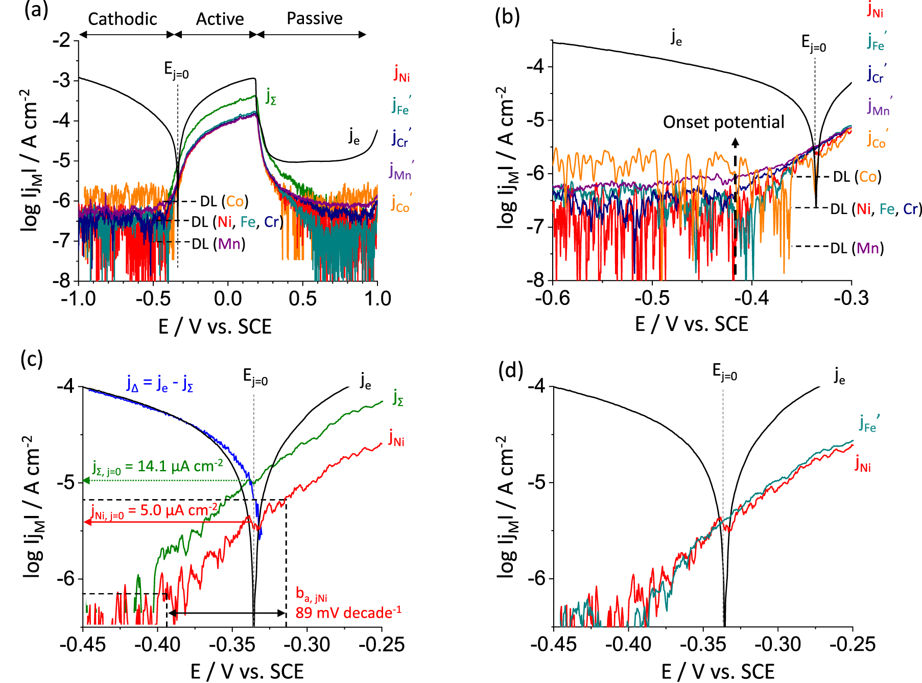
An elementally resolved potentiodynamic polarization curve, referred to as the AESEC linear sweep voltammetry (AESEC-LSV), for the Ni38Fe20Cr22Mn10Co10 MPEA in deaerated 2 M H2SO4 is shown in Fig. 3a. Expanded scale figures for the cathodic potential domain, and the potential near j=0 (E j=0 ) are given in Figs. 3b and 3c, respectively. Figure 3d shows a comparison between Ni (j Ni ) and normalized Fe dissolution rates (jFe') in the same potential domain as Fig. 3c. All elements dissolved near E j=0 by a potential dependent mechanism as shown in Fig. 3.

Figure 3. (a) AESEC-LSV curve of the Ni38Fe20Cr22Mn10Co10 MPEA in deaerated 2 M H2SO4, (b) magnified cathodic potential domain, (c) and (d) potential domain near Ej=0 (Tafel domain). Note that only jNi, j∑ and jΔ are presented in (c) to better illustrate how to define the elemental Tafel slope (ba, jM ) and extrapolate elemental dissolution rates from the AESEC-LSV curve at Ej=0 (jM, j=0). In (a) and (b), the detection limits (DL) of each elemental dissolution rate signal are indicated in horizontal dashed lines.
Download figure:
Standard image High-resolution imageIn the cathodic potential domain (Fig. 3b), all elemental dissolution rates except Mn were under the detection limit when E < −0.43 V vs SCE. All alloying elements showed an onset dissolution potential close to −0.43 V vs SCE, more negative than the E j=0 (−0.34 V vs SCE). For E > −0.43 V vs SCE the logarithm of each elemental dissolution rate is almost linear with the applied potential near E j=0 .
All elemental dissolution rates showed active-passive transition near 0.20 V vs SCE (Fig. 3a). An abrupt drop in current density and elemental dissolution rates near 0.2 V vs SCE may be attributed to the formation of the less soluble sulfate/oxide species or crystallization of dissolution products rapidly reaching supersaturation at the interface, 55,56 which is not predicted by thermodynamic simulation of pure metals in Fig. 1. The sum of instantaneous elemental dissolution rates (∑ j M = j ∑ ) is presented in Figs. 3a and 3c, indicating the total elemental current density equivalent to the alloy dissolution rate for cations in solution. In the active potential domain (E j=0 < E < 0.20 V vs SCE), some type of film (corrosion product) formation collecting alloying elements is implicated as j ∑ < j e . The corrosion product formed in this potential domain is probably a less protective transition metal sulfate that accounts for some elements that oxidize but that do not dissolve in solution. The Fe-based sulfate film in the active potential domain is reported to be porous and does not have the slow ion transport properties of a Fe-based oxide such as hematite, so as to be rate limiting. 8,26,57–59 For pH above a depassivation pH of each alloying element, corrosion may be determined by the characteristics of the corrosion product. For pH below the depassivation pH, the alloy potential may shift to the active-passive potential domain resulting in active dissolution. 58 In 2 M H2SO4 near E j=0 (or E oc ), the transition metals may all form metal sulfates with roughly similar high solubilities for Ni, Cr, Co, and Mn sulfates. However, for FeSO4, the molar solubility (i.e., 0.03 mol kg−1 in 10 mol kg−1 H2SO4) 58,60 is approximately 40 times lower than that of NiSO4 (i.e., 1.7 mol kg−1 in 10 mol kg−1 H2SO4). 58,61 Thus, the Ni-Fe-Cr-Mn-Co MPEA may form a FeSO4-like film near E j=0 in H2SO4. The charge unaccounted by the AESEC in this potential domain is 386 mC cm−2, calculated by a mass–charge balance (j Δ = j e - j ∑ ) assuming that the cathodic current is negligible. This relatively large charge may be attributed to formation of a layer on the alloy surface of the less soluble FeSO4. A slight selective Fe dissolution is indicated near E j=0 as j Fe ' > j Ni highlighted in Fig. 3d, similar to the open circuit dissolution previously discussed in Fig. 2. It may be attributed to chemical dissolution of the FeSO4 formed instantaneously on the surface when the sample is in contact with the H2SO4 electrolyte. In this case, the composition of the surface would have been altered resulting in a slightly higher Fe dissolution rate than a congruent level.
In the passive potential domain (0.20 V < E < 0.97 V vs SCE), all elemental dissolution rate signals decreased to the detection limit, almost independent of the applied potential, while the electrical current density was approximately 10 μA cm−2. The results also suggest that some anodic charge was devoted to the formation of the less soluble species including metal oxide/sulfate indicated by j ∑ < j e .
In Fig. 3c, log ǀj M ǀ vs E is expanded near E j=0 to determine the elemental Tafel slope from the AESEC-LSV curve. In the cathodic potential domain, cathodic current density (j c ) may be estimated as j c = j Δ = j e − j ∑ when assuming that the formation of non-dissolved species is negligible. In Fig. 3c, only j Ni , j ∑ and j Δ are presented as examples, and the same analysis was carried out for the other elements not shown in Fig. 3c. It should be noted that determining the Tafel slope for potentials more negative than the E j=0 is extremely difficult from the conventional LSV curve, whereas a slope from the log ǀj Ni ǀ vs E of the AESEC-LSV curve shows linear behavior for over an order of magnitude current range (i.e., 1 to over 10 μA cm−2), including potential domain more negative than the E j=0 . The determination of the elemental Tafel slope from j Ni is indicated with dashed lines in Fig. 3c as an example, giving 89 mV decade−1. Other elemental Tafel slopes (ba, jM ) were also determined from j M , summarized in Table I. These values are compared with the ba, jM determined from AESEC-EIS using elemental Lissajous plot discussed in the next section.
Table I. The elemental Tafel slopes (ba, jM ) determined both from AESEC-LSV curve (Fig. 3) and elemental Lissajous plot from AESEC-EIS (Fig. 6 and Eq. 10). The ba, jM values of a 304 stainless steel measured in the same electrolyte are presented for comparison. 44
| Ni38Fe20Cr20Mn10Co10 | 304 stainless steel 44 | ||
|---|---|---|---|
| 2 M H2SO4 | 2 M H2SO4 + 0.2 M NaCl | ||
| ba, jM | AESEC-LSV, ba, jM (Fig. 3) | AESEC-EIS, ba, jM (Fig. 6) | AESEC-LSV ba, jM |
| mV decade−1 | |||
| Ni | 89 ± 3 | 96 ± 1 | 68 |
| Fe | 78 ± 1 | 81 ± 4 | 59 |
| Cr | 87 ± 1 | 87 ± 5 | 60 |
| Mn | 101 ± 1 | 114 ± 5 | 65 |
| Co | 71 ± 5 | 76 ± 7 | — |
| ∑ j M (j ∑ ) | 80 ± 1 | 73 ± 3 | — |
The anodic elemental Tafel equation may be calculated by linear fitting of j M vs E curve in Fig. 3. For example, j Ni vs E from the linear fitting in the Tafel domain is obtained as:

Eq. 8 can be expressed as the anodic Ni Tafel equation:

where ET indicates a reference potential, and jT Ni is an equivalent Ni dissolution rate at ET. Using the values obtained in the open circuit dissolution from Fig. 2, jT Ni = j Ni, oc = 6.1 μA cm−2 and ET = E oc = −0.32 V vs SCE, the E in Eq. 9 gives 0.144 V, validating the linear fitting result in Eq. 8. The elemental anodic Tafel equations for the other elements obtained by linear fitting from Fig. 3 are given in Table II. It demonstrates that the spontaneous elemental dissolution (corrosion) rates can be simply estimated from the open circuit AESEC measurement which again gives complementary information to the conventional LSV electrochemical measurement.
Table II. Elemental dissolution rates extrapolated from the AESEC-LSV from Fig. 3 (j M, j=0 ) and measured during open circuit measurement from Fig. 2 (j M, oc ). The elemental Tafel equation is also provided from the linear curve fitting of Fig. 3 in Tafel domain. For Fe, both j Fe, j=0 and j Fe, oc may be slightly underestimated given that some of the Fe(II) is present in the form of less soluble FeSO4.
| M | j M, j=0 from Fig. 3 | j M, oc from Fig. 2 | E = ET + ba, jM log(j M /jT M ) |
|---|---|---|---|
| μA cm−2 | V vs SCE | ||
| Ni | 5.0 | 6.1 ± 0.8 | E = ba, jNi log(j Ni ) + 0.145 |
| Fe | 3.8 | 4.2 ± 0.3 | E = ba, jFe log(j Fe ) + 0.166 |
| Cr | 5.5 | 6.0 ± 0.5 | E = ba, jCr log(j Cr ) + 0.163 |
| Mn | 1.5 | 1.7 ± 0.1 | E = ba, jMn log(j Mn ) + 0.276 |
| Co | 1.1 | 1.1 ± 0.3 | E = ba, jCo log(j Co ) + 0.101 |
| ∑ j M (j ∑ ) | 16.9 | 19.1 ± 0.6 | E = ba, j∑ log(j ∑ ) + 0.119 |
The E j=0 (−0.34 V vs SCE) in Fig. 3 is close to the E oc (−0.32 V vs SCE) measured in Fig. 2. The slight difference is probably due to the activated and changing surface composition in 2 M H2SO4. In this case, it is of interest to compare the extrapolated elemental dissolution rates at E j=0 (j M, j=0 ) with the spontaneous elemental dissolution rates measured during open circuit dissolution (j M, oc ). As an example, the extrapolated j Ni, j=0 at E j=0 from the AESEC-LSV curve (straight arrow in Fig. 3c) yields 5.0 μA cm−2 while the j Ni, oc at a near steady state (500 s < t < 600 s) in Fig. 2 is 6.1 ± 0.8 μA cm−2. The extrapolated j M, j=0 and j M, oc values of each alloying element are summarized in Table II. The correlation between the j M, j=0 from the AESES-LSV (x-axis) and the j M, oc from AESEC open circuit experiment (y-axis) for all the alloying elements is presented in Fig. 4 showing a very good linear relationship between these two. This result demonstrates that the spontaneous elemental corrosion rates can be predicted by extrapolating the AESEC-LSV curve. This also suggests that conventional mixed potential theory 62 may be applied to estimate the elemental level spontaneous dissolution rates for each element in complex alloys using the AESEC-LSV methodology.

Figure 4. The relationship between jM, oc obtained from spontaneous dissolution in Fig. 2 (y-axis) at Eoc and extrapolated jM, j=0 from the AESEC-LSV curve of the Ni38Fe20Cr22Mn10Co10 MPEA at Ej=0 in Fig. 3 (x-axis). The dashed line indicates 1:1 relation.
Download figure:
Standard image High-resolution imageIt is interesting to note that the rank order of the elemental dissolution rates in mol cm−2 s−1 (Eqs. 5 and 6) near E j=0 follows the same order as the alloy composition. This is with the exception that there are slightly higher Fe and lower Co dissolution rates with respect to the alloy composition. This is not predictable in a straight forward manner from obvious thermodynamic nor kinetic considerations such as anodic over-potential relative to the electrode potential for elemental oxidation shown in Fig. 1. The cations selected for each element are the most stable form of that element in 2 M H2SO4 at E j=0 (or E oc ). The anodic over-potential at E j=0 is quite different for each element. For instance, Mn showed low j Mn, oc and j Mn, j=0 values in accordance with atomic composition whereas Mn oxidation occurs at the highest estimated anodic over-potential (1277 mV). This indicates the complexity of the system.
The sum of elemental dissolution rate (j ∑ ) may give a total corrosion rate of a system in the active potential domain. The extrapolated j ∑, j=0 from the AESEC-LSV curve (dotted arrow in Fig. 3c) is 16.9 μA cm−2 again comparable to j ∑, oc = 19.1 μA cm−2 obtained from open circuit dissolution (Table II), which may also be used to estimate the total corrosion rate of an MPEA.
Elemental dissolution kinetics: AESEC-EIS at E oc
The elemental current densities (j M ) and the corresponding electrical current density (j e ) measured during AESEC-EIS experiments for the Ni38Fe20Cr22Mn10Co10 MPEA in deaerated 2 M H2SO4 at E oc are shown in Fig. 5a. The open circuit measurement was conducted for the first 1000 s, then the potentiostatic EIS at E oc was carried out. It can be seen that the current density in high-frequency domain is predominantly capacitive, and that as the frequency decreases the current becomes dominated by metal dissolution into the solution indicated by the oscillation of the j M . The j M , j e , and E profiles at f = 0.0056 Hz are magnified in Fig. 5b to better illustrate the oscillation of each signal a . All j M showed a near in-phase oscillation with the applied sinusoidal potential and the resulting j e , indicating a direct relationship between the formation of the oxidized dissolved species and the potential excitation. Concerning the alloying elements, selective Fe dissolution was detected while Cr, Mn and Co dissolved close to their congruent levels, as previously observed in Fig. 2. All elements dissolved at this potential as thermodynamically predicted from Fig. 1. The formation of less soluble oxidized species as a result of the slightly more positive applied potential (E oc ≈ −0.32 V vs SCE) than the E j=0 (−0.34 V vs SCE) is indicated. The center of j e , non-linear dashed line shown in Fig. 5a obtained by an average value between the highest and lowest points of j e , was not 0 and increased above 0 at the end of the measurement. This indicates that the net reaction was anodic, assuming there was no capacitive contribution. It should be noted that j ∑ < j e during AESEC-EIS at E oc , possibly due to the formation of sulfate. Another indication of the less soluble species formation during AESEC-EIS at E oc is the decrease in elemental dissolution rates after the EIS as compared to the first open circuit measurement.

Figure 5. (a) AESEC-EIS of the Ni38Fe20Cr22Mn10Co10 MPEA in deaerated 2 M H2SO4 at Eoc. Spontaneous dissolution was measured for the first 1000 s, then a potentiostatic AESEC-EIS experiment was conducted at the final Eoc. (b) A close-up figure at f = 0.0056 Hz. Note that all the normalized elemental current densities are multiplied by 3 in (b) for the ease of comparison with je.
Download figure:
Standard image High-resolution imageThe elemental Lissajous plot at f = 0.0056 Hz from the AESEC-EIS at E oc is presented in Fig. 6 showing the relationship between the AC potential perturbation and elemental dissolution rates. All elemental dissolution rates show oval shapes indicating possible capacitive current and reasonable pseudo-linearity. It should be noted that the slope ∆E/j e in Fig. 6a is similar in magnitude to a polarization resistance (R p ) at f → 0 (e.g., ∼ 400 Ω cm2) where ΔE is the difference between the most positive and negative AC potentials above and below E oc . The slopes ∆E/j M yield elemental values of R p where ∆E/j ∑ = ∆E/j e if all elements that have oxidized are dissolved and detected by AESEC. However, this is not the case implying that a corrosion product has formed such as a transition metal oxide or sulfate film that does not dissolve in solution, indicated by j ∑ < j e in Fig. 5. Thus, some of the metallic elements, particularly Fe, were oxidized but not dissolved in the solution as also indicated by the LSV in Fig. 3. The corrosion includes a portion of metal oxidized and not measured by AESEC-EIS (Fig. 5) consistent with AESEC-LSV (Fig. 3).
From Fig. 6, the elemental Tafel slopes (ba, jM ) may be determined as:

where j M + and j M − are the dissolution rates of M at the most positive and negative potentials in the Lissajous plot, respectively. The ba, jM values obtained from Eq. 10 are summarized in Table I, and compared with the previously determined ba, jM values from the AESEC-LSV curve in Fig. 3 showing a good agreement between the two different methods. The low ba, jFe value for Fe may account for the selective dissolution of Fe during the open circuit dissolution (Figs. 2 and 5).

Figure 6. (a) Elemental Lissajous plot of the Ni38Fe20Cr22Mn10Co10 MPEA obtained from Fig. 5 at Eoc and f = 0.0056 Hz; and (b) decomposed plot by each alloying element.
Download figure:
Standard image High-resolution imageElemental kinetics: AESEC-EIS at a passive potential
The elemental dissolution kinetics were significantly different during electrochemical passivation conducted at a potential in the passive potential domain, 0.60 V vs SCE, as shown in Fig. 7. The passive potential was chosen from the AESEC-LSV (Fig. 3). The dissolution transients for the initial 1500 s and in the low-frequency domain (2700 s < t < 6500 s) are magnified in Figs. 7b and 7c, respectively. A constant potential of 0.60 V vs SCE was applied to the sample from t = 0. Following the potentiostatic hold for 1500 s, the AESEC-EIS was carried out at 0.60 V vs SCE. Selective dissolution of Mn, Cr and Fe were observed during AESEC-EIS at 0.60 V vs SCE as shown in Fig. 7 while the Ni dissolution rate was only slightly above the detection limit (0.13 μA cm−2), and Co was under the detection limit. Recall that all elemental dissolution rates were under the detection limits in the passive potential domain near 0.6 V vs SCE in the AESEC-LSV curve (Fig. 3). It should be also noted that the j e during the potentiostatic experiment in Fig. 7a showed a typical trend of decaying with time, which may indicate passive film thickening that reduces the potential drop across either the passive film itself, at the passive film/metal interface or the passive film/solution interface as the passive film grows. 63,64 All elements showed some degree of non-congruent dissolution during passivation as j M ' ≠ j Ni . The j Cr ' and j Fe ' showed decaying trends in Fig. 7a similar to j e , an indicative of the contribution towards passivation of these elements. 65 The dissolution rate of Cr was 15 at%, and that of Fe was 14 at% of the total dissolution rate, lower than their congruent dissolution level. However, j Mn ' increased during the measurement with a significantly higher rate than j Ni . The j Mn ' increased even after potential release to the open circuit at the end of the experiment, which may indicate the chemical dissolution of the Mn-based passive film formed during passivation experiment. This is supported by the increase in open circuit potential after potential release (+0.36 V vs SCE, Fig. 7a) compared to the open circuit potential of the system without passivation procedure (−0.32 V vs SCE, Fig. 2). Both j Co ' and j Ni showed dissolution transient during the first 1500 s of the potentiostatic hold (Fig. 7b) and were close to the detection limit during AESEC-EIS (Fig. 7c). This may be due to the formation of stable Ni- and Co-based passive films or accumulation of un-oxidized Co or Ni metal at the passive film/metal interface. This has been suggested by 3-D atom probe tomography on the same alloy, albeit at T = 120 °C and 300 °C. 66 It was confirmed that Cr and Fe contribute to passive film formation in combination with some simultaneous dissolution, in agreement with the previous observation on the same alloy at pH = 4.0, with 0.1 M NaCl during a potentiostatic hold experiment at a passive potential. 34 In the passive film, Mn may be also present given that the dissolution behavior reached a quasi-steady state for t > 5000 s. However, such a film would not be stable as the Mn dissolution rate was higher than other alloying elements and did not show a decaying profile with time, similar to the previously observed case for the same MPEA at pH = 4.0 in 0.1 M NaCl. 34,35

Figure 7. (a) AESEC-EIS of the Ni38Fe20Cr22Mn10Co10 MPEA in deaerated 2 M H2SO4 at 0.60 V vs SCE. A constant potential of 0.60 V vs SCE was applied for the first 1500 s, then potentiostatic AESEC-EIS was conducted at the same potential. Close-up figures are given for the first 1500 s for the potentiostatic hold in (b) and for the low-frequency EIS domain in (c).
Download figure:
Standard image High-resolution imageIt should also be noted that no potential dependent oscillation was observed for all elemental dissolution rates during AESEC-EIS at 0.60 V vs SCE, different from that at E oc shown in Fig. 5. One proposal is that the elemental dissolution occurred through a chemical reaction involving the dissolution of the passive film with time that is not excited or triggered by the applied AC potential. 40,42 Another possibility is that elemental dissolution is nearly independent of potential during passivation. The j e decayed as a function of time at 0.60 V vs SCE and was substantially more independent of potential than in the case of active dissolution near E j=0 (Fig. 3), hence, it was not responsive to the small potential perturbation.
Conventional potentiostatic EIS data obtained during AESEC-EIS experiments at E oc and at 0.60 V vs SCE are presented in Figs. 8a and 8b, respectively. Simplified model circuits for the two potential domains are provided in the inset of each Nyquist plot, and fitting results are provided in stacks.iop.org/JES/169/081507/mmedia Supplementary data. The outmost component (CPE 1 /R 1 ) in the inset of Fig. 8 is the double layer contribution. At 0.60 V vs SCE (Fig. 8b), a porous passive film model circuit 35,67 is suggested, probably due to the selective dissolution of Mn, Cr and Fe as previously shown in Fig. 7. In either case, a two or three time-constant process is indicated by the model circuit fitting which may indicate of a layered film as previously observed in similar systems. 34,35,54,68 The CPE parameters of the double layer contribution were calculated from the graphical analysis of the EIS spectra 47,48 as described in the experimental section. At E oc (Fig. 8a), Q dl = 86.5 × 10⁻⁶ F s(α−1) cm−2, and α dl = 0.90; and at 0.60 V vs SCE (Fig. 8b), Q dl = 50.1 × 10⁻⁶ F s(α−1) cm−2, and α dl = 0.90. Using Cole-Cole representation of the real and imaginary capacitance, 69 the effective capacitance of the passive film (C δ ) was obtained from the high-frequency boundary in the real component of the capacitance. Note that the total impedance as well as the capacitance have been corrected as described in Eqs. 2 and 3, taking into account the effect of double layer capacitance. 47,48 At E oc , C δ = 3.5 × 10⁻⁶ F cm−2, and at 0.60 V vs SCE, C δ = 1.9 × 10⁻⁶ F cm−2. Notably, Fig. 8a shows that R p at f → 0 Hz is about 305 Ω cm2 in close agreement with ∆E/j e in Fig. 6.

Figure 8. Nyquist plots of the Ni38Fe20Cr22Mn10Co10 MPEA obtained during AESEC-EIS (a) at Eoc (from Fig. 5), and (b) at 0.60 V vs SCE (from Fig. 7). Equivalent model circuits are given in the inset of each figure. The symbols represent the measured data points and the solid lines represent the fitting results. Note that the Nyquist plots presented here possessed a solution resistance of Re = 29 Ω cm2 which has been corrected.
Download figure:
Standard image High-resolution image
Discussion
Active dissolution
In this work, elementally resolved dissolution kinetics of a multi-principal element alloy Ni38Fe20Cr22Mn10Co10 was investigated via AESEC-EIS in the Tafel, active and passive potential domains in 2 M H2SO4. The elemental Tafel slopes (ba, jM ) were obtained both from the AESEC-LSV curve and elemental Lissajous plot from AESEC-EIS which suggested different elemental dissolution rates of each alloying element near E j=0 . The elemental dissolution (corrosion) rates were either directly measured by the AESEC open circuit experiment (j M, oc ), or extrapolated from the AESEC-LSV at E j=0 (j M, j=0 ). The elemental Tafel slopes obtained in this work were slightly different from the previous studies reporting a range from 59 ∼ 68 mV decade−1 for 304 stainless steel, 44 91 mV decade−1 for Fe and 76 mV decade−1 for Cr contained in the Fe-Cr alloys, 70 and approximately 60 mV decade−1 for pure Fe 71,72 in acidic solutions. The Tafel slope contains fundamental information on the reaction mechanism giving the rate-determining step in multi-step reactions, and the role of adsorbed intermediates and films during active dissolution. The generally lower Tafel slopes in the case of Ref 44 than those obtained in this work could be due to the presence of Cl− in the electrolyte for Ref 44 resulting in more rapid elemental dissolution. For the Ni38Fe20Cr22Mn10Co10 MPEA investigated in this work, ba, jM varied from 71 to 114 mV decade−1 depending on the element whereas each elemental dissolution occurred in a similar rate to each other for the 304 stainless steel (59 ∼ 68 mV decade−1). 44
The fundamental question is whether the elemental dissolution ranking is predictable based on thermodynamic 18,19,73–75 and/or kinetic considerations in an MPEA given the expectation of modified metallic bonding considerations such as provided by first and second nearest neighbors in either a random solid solution or an alloy with short-range order. Exact comparison is difficult, but data on the dissolution rate of each element in 0.5 M – 2 M H2SO4 compared to the same element in high purity form is worth comparing. Regarding kinetics, the overall E oc and the active potential domain experienced by this MPEA in H2SO4 imposes various anodic over-potentials on each element depending upon its oxidation half-cell potential (or that of a modified electrode potential for an MPEA based on nearest neighbors). It can be argued that the thermodynamic driving force represented by the over-potential as well as the activation energy for the oxidation of each element depends on the FCC structure, and short-range order dictating nearest neighbors and bonding. These factors affect both the chemical potential of solid metal elements. Bonding strength affects the activation barrier height for bond cleavage. 76 A simple way to assess this is based on comparison of the melting temperature (Tm,M) of each element when there are nearby "like" elements compared to "unlike" elements. It is assumed that all elements are oxidized to form a cation which is stable in the 2 M H2SO4 solution. The question is whether alloying elements can break the bond and become oxidized and solvated more easily or less easily in the MPEA. Table III summarizes Tm,M of each element, and anodic over-potential (η) vs E oc (−0.32 V vs SCE) determined from Fig. 1 at C M = 10–6.5 M. A lower Mn dissolution rate (higher ba, j Mn ) near E oc (and E j=0 ) for the MPEA could be explained by "unlike" nearest neighbors which all have higher Tm,M. 75 In contrast, Cr is surrounded by elements with a lower Tm,M compared to pure Cr surrounded by other Cr atoms. In the absence of Cr-Cr clustering, Cr would be expected to dissolve as Cr(III) at relatively high rates given this atomistic condition and the high η (998 mV, Table III). Co and Ni have the lowest η and they are in an environment with both lower (e.g., Mn) and higher Tm,M (e.g., Fe and Cr) elements. The exchange current densities of the pure metals in H2SO4 reported from literatures are provided in Table III, giving the ranking order of Ni ≈ Fe > Cr > Mn. In this work, the spontaneous dissolution rates expressed as equivalent current densities were in the order of Cr ≈ Ni > Fe > Mn > Co, different from the comparisons of the exchange current density. It should be noted that extrapolating the log ∣j M ∣ vs E plot to an estimated exchange current density from the AESEC-LSV result in Fig. 3 is difficult since the detection limit of each elemental dissolution rate is greater than the actual elemental exchange current density and there is uncertainty in the elemental concentration (CM) at the surface. Therefore, the exchange current density rankings may not be accessible.
Table III. Melting temperature of metal M (Tm,M), andic over-potential η vs E oc (−0.32 V vs SCE) determined from Fig. 1 at C M = 10–6.5 M. The j M, oc and j M, j=0 values obtained in this work are compared with the exchange current densities reported for the pure metals in the literature.
| M/M(z+) | Tm,M | η vs E oc | Ni38Fe20Cr20Mn10Co10 in 2 M H2SO4 | Pure metals in the literature | |
|---|---|---|---|---|---|
| j M, oc | j M, j=0 | Exchange current density | |||
| °C | mV | A cm−2 | A cm−2 | A cm−2 | |
| Ni/Ni(II) | 1453 | 341 | 6.1 × 10⁻⁶ | 5.0 × 10⁻⁶ | 2.5 × 10⁻⁶ (1 N H2SO4 + 1 M Na2SO4) 77 |
| Fe/Fe(II) | 1538 | 578 | 4.2 × 10⁻⁶ | 3.8 × 10⁻⁶ | 1.6 ∼ 5.5 × 10⁻⁶ (0.5 M H2SO4, 22 °C) 78 |
| Cr/Cr(III) | 1907 | 998 | 6.0 × 10⁻⁶ | 5.5 × 10⁻⁶ | 4 × 10⁻⁷ 1 N H2SO4, 25 °C 79 |
| Mn/Mn(II) | 1246 | 1277 | 1.7 × 10⁻⁶ | 1.5 × 10⁻⁶ | 1.3 × 10⁻¹¹ (1 mol kg−1 H2SO4) 80 |
| Co/Co(II) | 1495 | 383 | 1.1 × 10⁻⁶ | 1.1 × 10⁻⁶ | — |
The elemental dissolution rates (in mol cm−2 s−1, using Eqs. 5 and 6) were found to rank from fastest to slowest in the same order as alloy concentrations with some deviations from this trend, such as the selective dissolution of Fe near E oc . This trend was modified by the formation of a metal oxide or sulfate which captured, in particular, some of the oxidized Fe.
Passive dissolution
For the same MPEA in a pH = 4.0, 0.1 M NaCl solution, no thermodynamically stable oxide at 0.60 V vs SCE was predicted by Wang et al. 18 In that condition, the passivation is likely due to formation of metastable phases. The extension of stable oxides observed at pH = 4 suggested either a corundum or possibly a spinel solid solution. 18 Mn showed intense selective dissolution during the AESEC-EIS at a passive potential of 0.60 V vs SCE (Fig. 7), similar to a previously observed potentiostatic experiment at 0.10 V vs SCE for the same MPEA in a 0.1 M NaCl, pH = 4.0 solution. 35 The oxidized Mn was characterized by ex situ XPS using 3p core level analysis, indicating that Mn-based oxidized species were present in the passive film. 35 However, the presence of Mn in the passive film of the Ni, Fe, Cr, and Mn containing MPEAs caused a decrease in corrosion resistance above 5 at% Mn as evidenced by the electrochemical analysis. 21,35,81,82 The j Mn ' in Fig. 7b showed a typical passivation trend for the first 500 s, then the Mn dissolution rate progressively increased with time (Figs. 7a and 7c) which may indicate less stable Mn-based passive film formation than other elements. For the elementally resolved analysis, however, the behavior of the individual elements does correspond with the total current density implying accumulation of cations in oxidized surface films, as shown in Fig. 7. A similar example has been previously reported for the AA2024 alloy where Mg actively dissolved in the passive potential domain and showed a passivation trend in the active potential domain. 83
The excess Cr relative to Ni at the surface,  was estimated by mass balance as:

where X
Cr
and X
Ni
are mass fractions of Cr and Ni, respectively. For the AESEC-EIS at E
oc
(Fig. 5),  = 3.1 nmol cm−2; and at 0.60 V vs SCE (Fig. 7),
  = 6.8 nmol cm−2 at the end of each experiment. The estimated thickness values assuming uniform formation of Cr2O3 (density = 5.22 g cm−3) were 0.9 nm at E
oc
, and 2.0 nm at 0.60 V vs SCE, respectively. Based on the same assumption, the effective passive film thickness (δ) using C
δ
obtained from Cole-Cole representation of the EIS results was estimated as:
= 6.8 nmol cm−2 at the end of each experiment. The estimated thickness values assuming uniform formation of Cr2O3 (density = 5.22 g cm−3) were 0.9 nm at E
oc
, and 2.0 nm at 0.60 V vs SCE, respectively. Based on the same assumption, the effective passive film thickness (δ) using C
δ
obtained from Cole-Cole representation of the EIS results was estimated as:

where ε is the dielectric constant of the Cr2O3 (ε = 12.6 from 84 ) and ε 0 is the vacuum permittivity (8.85 × 10⁻¹⁴ F cm−2), giving δ = 3.2 nm for E oc , and δ = 5.8 nm for 0.60 V vs SCE, respectively. The passive film thickness values estimated from EIS were thicker than those obtained from mass balance, which may indicate the presence of sulfates/oxides other than Cr-based. A possible formation of less soluble Fe sulfate would also be responsible for the difference between the EIS estimation and the AESEC mass balance. In the passive potential domain (Fig. 7), the j Ni and jCo ' were close to the detection limit at the end of the experiment, different from Fig. 1 where soluble Ni(II) and Co(II) are predicted to be thermodynamically stable. This may be due to the formation of a Ni or Co-based passive film, or a modified metallic layer enriched with Ni. 34,66
In summary, elemental specific dissolution could be monitored by AESEC-LSV but not by AESEC-EIS to ascertain elements dissolving in solution when in the passive potential range using the detection limits available in this study. Elements oxidized but not dissolved (i.e., present in the passive film) could be ascertained by AESEC mass-charge balance.
Elemental contribution to the impedance response
The real part of the electrochemical impedance from each j M , Z r (j M ), at the low-frequency domain at E oc are provided in Table IV obtained as:

where ϕ is the R e corrected phase angle. The elemental dissolution impedance was not in a simple series relationship because Z r − R e < Z r (j M ). Assuming a bilayer passive film model suggested for a Ni-Fe-Cr-Mn-Co MPEA in H2SO4 with outer Co- and Fe-based passive film layer and inner Cr-, Ni- and Mn-based passive film layer, 54 the effective total impedance calculated from Eq. 13 gives 321 Ω cm2, close to the measured Z r − R e value of 305 Ω cm2 obtained from the potentiostat. The slight difference may be due to the non-negligible cathodic current or to the contribution of less soluble species to the total current density. This implies that corrosion products such as transition metal sulfates are formed which do not dissolve in solution as indicated by j ∑ < j e in the active potential domain in the LSV (Fig. 3) and EIS (Fig. 5) experiments.
Table IV. The elemental real part impedance (Z r (j M )) calculated from Eq. 13. The elemental Tafel slopes (ba, jM ) and elemental dissolution rates extrapolated at Ej=0 (j M, j=0 ) are also provided.
| Ni | Fe | Cr | Mn | Co | Z r — R e | |
|---|---|---|---|---|---|---|
| Z r (j M ) / Ω cm2 at f = 0.0056 Hz | 316 | 390 | 395 | 386 | 450 | 305 |
| ba, jM / mV decade−1 (AESEC-EIS) | 89 | 78 | 87 | 101 | 79 | — |
| j M, j=0 / μA cm−2 (AESEC-LSV) | 5.0 | 3.8 | 5.5 | 1.5 | 1.1 | — |
In Table IV, the j M, j=0 and ba, jM values from Tables I and II correlate with Z r (j M ). A relatively high Z r (j M ) value corresponding to a low j M, j=0 value was obtained for all elements except Cr. This indicates that the Z r (j M ) may be correlated with the interaction between the intensity of the elemental dissolution rate (j M, j=0 ) and the change of the elemental dissolution rate with the potential (ba, jM ).
Summary
- The direct dissolution of each alloying element from Ni-Fe-Cr-Mn-Co MPEA surface to 2 M H2SO4 electrolyte is indicated by an in-phase elemental dissolution rate responding to the applied sinusoidal potential. This was determined from AESEC-EIS analysis at E oc .
- No oscillation of the elemental dissolution rate signal was detected by AESEC-EIS in the passive potential domain. This indicates the dominant chemical dissolution of the outer layer of the passive film weakly coupled to metal oxidation at the metal/passive film interface with a highly resistive potential-current relationship nearly independent of potential excitation.
- Spontaneous elemental dissolution rates measured by AESEC showed nearly 1:1 relationship with elemental dissolution rates extrapolated from AESEC-LSV at E j=0 , which sheds light on element-specific dissolution tendencies and the propensity for selective dissolution.
- A marginally protective Fe-based sulfate formation is indicated by the AESEC-LSV result in the active potential domain where the anodic oxidation reaction is consistent with a charge-transfer process and follows Tafel behavior.
- A less stable Mn-based passive film formation is indicated during application of an applied potential in the passive potential domain. The selective dissolution rate of Mn at this potential increased with time whereas other alloying element showed typical passivation trends.
- The active and passive dissolution of the individual alloying elements was a complex function of kinetic and thermodynamic factors. When all elemental dissolution rates in an active potential domain were controlled by a charge-transfer mechanism, the rates scaled with alloy composition. The exception was in the case of Fe which showed slight selective dissolution.
Acknowledgments
The research conducted by A. Y. Gerard, J. R. Scully, P. Lu, J. E. Saal and J. Han was supported as part of the Center for Performance and Design of Nuclear Waste Forms and Containers (WastePD), an Energy Frontier Research Center (EFRC) funded by the U.S. Department of Energy (DOE), Office of Science, Basic Energy Sciences (BES), under award #DE-SC0016584. K. Ogle and the AESEC experiments conducted by J. Han were supported by the Agence Nationale de Recherche, grant #ANR-20-CE08-0031 (Tapas 2020).
Footnotes
- a