
Abstract
Aqueous fluoride solutions underpin much of silicon processing because they are used to strip oxide layers and for cleaning. Depending on their composition and reaction conditions they can be used to create either flat, hydrogen-terminated surfaces or nanocrystalline porous silicon. Nonetheless, confusion reigns regarding the identity and quantity of different solution species as a function of the formal concentration of HF and other additives. The literature is critically surveyed, data and results are reanalyzed, and analytical expressions are derived that allow for the calculation of solution species activities. Above  , fluoride solutions are highly nonideal. It is shown that the main constituents of acidic fluoride solutions are
  ,
,  , HF,
, HF,  , and
, and  in the range of
  and even as high as
  . In these concentration ranges the derived analytical expressions exhibit excellent and approximate agreement with experimental data, respectively. The nature of the HF species that exists in solution, whether it exists as a contact ion pair or as a solvated molecule, remains in doubt.
Export citation and abstract BibTeX RIS
Silicon electrochemistry1, 2 is extremely versatile and a great deal of work has been carried out in aqueous fluoride solutions. Fluoride solutions also serve as a workhorse in silicon wafer cleaning.3–5  is etched by fluoride solutions much more rapidly than Si. In the study of the mechanism of either
  etching6–11 or Si etching,12–16 it is important to understand the effects of solution composition in order to understand which solution species are actually involved in the reaction.17 Attempts to fit etch rates to the formal concentration of HF are of little mechanistic value because the concentrations of solution species vary with formal HF concentration in a highly nonlinear fashion. Nonetheless, studies appear regularly in reputable journals including this one in which solution equilibrium expressions are used incorrectly, either because of the expressions used or because the concentration ranges are inappropriate.
Given the centrality of fluoride solutions to silicon processing, it is surprising that so much confusion is encountered regarding the composition of fluoride solutions, but even in its pure form, HF is a notoriously difficult molecule to characterize.18, 19 Questions include both the nature and the quantity of fluoride species and how these vary with solution composition. I have reanalyzed and critically investigated the literature that exists concerning aqueous fluoride solutions and arrive at a best set of equilibria and their associated constants. Solution species activities are calculated numerically for a wide variety of solutions and these are fit to analytical expressions which can be used to determine the fluoride compositions of arbitrary solutions over specific ranges of formal concentration. One of the prime objectives of this work is to demonstrate the concentration range over which predictions of composition are accurate, approximate, or inappropriate.
Review of the Fluoride Solution Literature
In 1912 Pick20 suggested that the conductivities of aqueous HF solutions are consistent with the following two equilibria
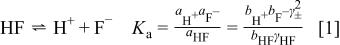
In the equilibrium expressions,  is the activity of species x,
  is the molality (moles per kg of solvent) of x, and
  is the activity coefficient of x. For solutions with formal concentrations of HF below
  and certainly no greater than
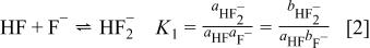
  , these two equilibria largely suffice to describe the main solution components. However, deviations at higher concentrations indicate that higher equilibria must also be considered.21, 22 McTigue and co-workers23, 24 demonstrated that the inclusion of a third equilibrium
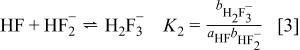
is required for quantitative work up to  HF solutions.
Numerous investigations of fluoride in water23–33 and water/ethanol34, 35 solutions have been made. A critical review of the literature up to 1984 was made by Hefter.31 Warren28 suggested the formation of the dimer  should be accounted for; however, no other corroboration for this species in solution can be found for the concentration range considered here (
 ,
,  ,
,  by weight). Dimers or even hexamers may exist in very concentrated solutions,23 and dimers have been detected spectroscopically in
  HF.36 There is no credible evidence for
  .37 The addition of ethanol to the solution changes the equilibrium constants dramatically,34, 35 but pure water solutions are dealt with here.
There is considerable interest in explaining the anomalously small acid dissociation constant for HF. One line of thought, that of Giguère and Turrell,38 posits that HF actually does dissociate strongly but that its interaction with water is so strong that it is bound in a contact ion pair,  . Spectroscopic measurements were used to establish that the
  ion pair or proton-transfer complex is a major species in HF(aq). This complex owes its remarkable stability to a strong hydrogen bond. Being ionic, yet electrically neutral, it can account both for the essentially complete ionization of HF in water and the apparent weakness of the dilute acid. The ionization process may be represented by the double equilibrium

Whereas the first equilibrium lies far to the right, the second corresponds only to about 15% dissociation. Both Raman and IR spectroscopy were used to assign the spectrum of  and to identify
  .
.
Laasonen and co-workers,39, 40 who performed Car-Parrinello molecular dynamics calculations on DF in  , agree with the interpretation of the IR bands observed by Giguère and Turrell.38 They used a 32-molecule liquid-water configuration in which one water molecule has been replaced by DF to model a deuterated aqueous solution. They found that the most appropriate way to describe solvated DF is to view it as a complex dynamically fluctuating between
  and
and  with the lifetime of the contact ion pair
  on the order of several picoseconds. Using time averages, they found that in a dilute
  solution the weights of the configurations
  ,
,  , and
, and  are 60:30:10, which is in line with the prediction made using
  and counting the first two configurations as undissociated DF. A similar picture is found for 50% HF.41
The formation of a contact ion pair is disputed by McTigue et al.23 Their potentiometric and conductometric data indicated quite high concentrations of HF exist in solution, both as individual molecules and hydrogen-bonded to fluoride ions. They believe that the reason for the lack of any clear spectroscopic evidence for nondissociated HF is more likely due to the broadening of the expected bands than to the absence of the molecules.
Ando and Hynes42 also questioned the formation of a contact ion pair. They performed a quantum Monte Carlo study of HF in water and cast doubt on the conclusion of Giguère and Turrell that the contact ion pair should be the primary fluoride species and the reason for the apparent weakness of HF. Ando and Hynes believe that contact ion pair formation (forward step in E1) is disfavored with a free energy of  . The break up of this into the free ions (forward step in E2) is thermoneutral. Thus, they posit that the weakness of HF is due to the endoergicity of the first step. This would mean that there should be no spectroscopic evidence for the contact ion pair as put forward by Giguère and Turrell. Ando and Hynes state, however, that both barriers (those associated with the forward reactions in E1 and E2) have values close to the accuracy of their method, and therefore, the height of the barriers could be reversed, even though they doubt this.
Derivation of Analytical Composition Expressions
A consensus has now formed24, 31 that reliable data for the determination of  at
at  have been measured by Wooster,43 Broene and De Vries,25 Ellis,44 Erdey-Gruz,45 Baumann,27 Kresge and Chiang,29 Hefter,31 and Braddy et al.24 As recommended by Braddy et al. , a value of
  is adopted here. Good data for the determination of
  and
and  has been measured by Braddy et al. ,24 and these data are used in conjunction with the three equilibria described previously to derive values of
  ,
,  and analytical expressions for the activities of
  , HF,
, HF,  ,
,  , and
, and  in a variety of solutions.
Braddy et al. have analyzed their data by fitting to the following expression (see original reference for details)
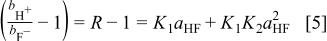
Their original analysis arrived at  . Reanalysis (see Fig. 1) of this data using nonlinear least squares fits yields a value of
  , which agrees within uncertainty. This compares to the values found by Broene and De Vries25 and Kresge and Chiang29
  , Davies and Hudleston21
  , and Baumann27
  . Braddy et al. 's value for the second equilibrium constant was
  , whereas this reanalysis yields
  . The set of equilibrium constants recommended in Table I yields a good description of the composition of solution up to a concentration of
  .
.
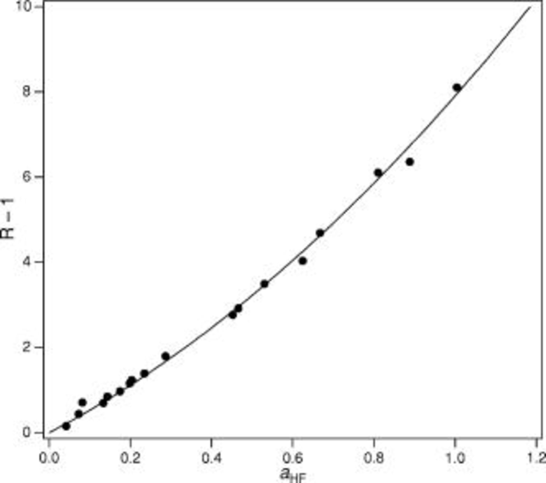
Figure 1. Reanalysis of the data from Ref. 24 for the determination of  and
and  .
.  is the ratio of the molalities of
  to
to  , and
, and  is the measured activity of HF.
Table I. Recommended values for the three equilibrium constants that describe aqueous solutions of HF from  .
.

|

|

| 5.0 |

| 0.58 |
To relate the activities to the formal concentrations added to make up the solutions, it is necessary to calculate the activity coefficients and molalities (given by  in Eq. 1, 2, 3). Fluoride solutions are highly nonideal except at the lowest concentrations; therefore, the use of concentrations for quantitative work is to be avoided, vide infra, above
  . The formal concentrations of each component added to the solution is defined here as
  ,
,  ,
,  , and
, and  . Hence, for any solution made up from a combination of water, HF, YF (
 e.g., Na, K, or
  ), HX (
 e.g., Cl), and
  , one obtains six simultaneous equations that must be solved to derive the equilibrium solution composition. The first three equations are provided by the equilibria 1, 2, 3, to which is added the water equilibrium

fluoride conservation

and charge balance

As all of the solutions considered here are acidic,  , and as a first approximation,
  is neglected in the charge balance equation. This approximation (as well as the introduction of the ammonia equilibrium where appropriate) were also tested directly but were found to be unimportant. Equations 1, 8 can be combined to yield

This leaves four equations and four unknown concentrations [HF],  ,
,  , and
, and  .
.  and
and  can then be back-calculated from Eq. 8, 6, respectively. The four equations are nonlinear and have no analytical solution, thus they were solved numerically using Mathematica. An iterative process was used in which the criterion for accepting a solution was that the ionic strength of the solution converged to better than 1 part in
  .
.
Confirmation of the goodness of the fitting procedure and equilibrium constants derived here is presented in Fig. 2 and 3. The values of  ,
,  , and
, and  are used to predict the molalities of
  and
and  in HF(aq). The predictions are excellent up to
  . In the region
  the predictions provide a fair representation of the solution compositions. The average deviation in the range
  is
is  for
for  and
and  for
for  . Therefore, even in this range, the agreement is still quite good. The disagreement in this range is comparable to the error that would be introduced simply by substituting concentration for activity in a
  solution of HF. In
  HF(aq),
  and
and  . Moreover, the activity coefficients change nonmonotonically with concentration as shown in Fig. 4. Therefore, even in dilute solutions, the use of concentrations instead of activities has inherent inaccuracies due to the highly nonideal nature of fluoride solutions. Any quantitative rate equation that uses concentrations instead of activities will similarly suffer from these inaccuracies.
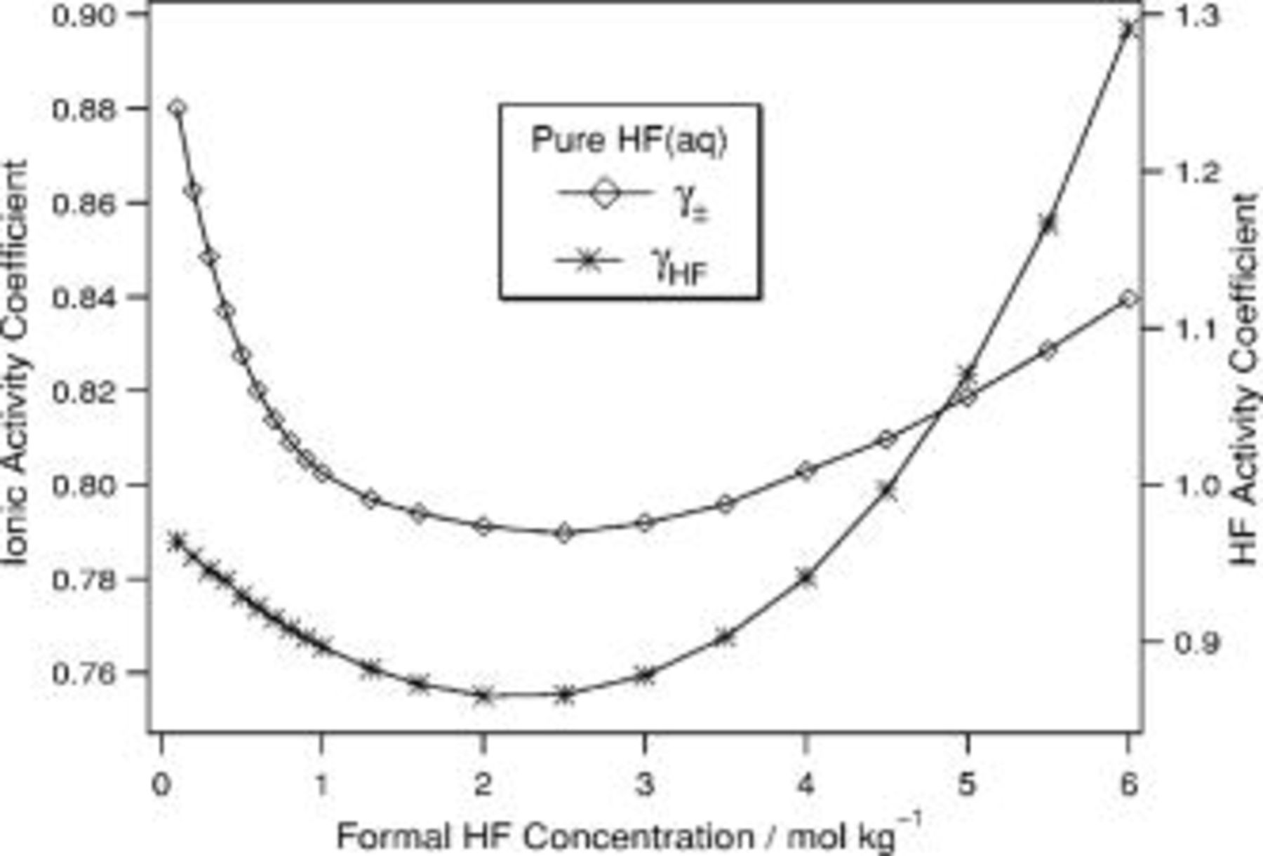
Figure 4. Calculated activity coefficients for ionic species, γ±, and HF,  , over the range of
  for aqueous HF.
The numerical approach described above was used to predict the concentrations of several classes of solutions. The range in which composition can be predicted with confidence is judged somewhat subjectively. It is seen in the pure HF solution (cf. Fig. 4) that as the numerical description of the solution composition begins to deviate from the measured values, the activity coefficient of HF begins to increase dramatically. This rough criterion of a rapidly increasing  has been used to assess the range of validity for the solutions treated below.
In Fig. 5, 6, 7, 8, 9 and 10 below, the activities of  , HF,
, HF,  ,
,  , and
, and  are presented. HCl is used as a specific example of a proton source but the
  ion plays no specific role in the results and could be replaced with other anions. Similarly, NaF could be replaced by KF or
  and the results would be the same. A common technical grade of
  contains
  ; therefore, calculations specific to this composition have been carried out. In many of these solutions, the activities change nonmonotonically, which may seem counterintuitive. Each curve has been fit to an analytical expression and the coefficients for these expressions are collected in Table II.
Table II. Coefficients of the analytical expressions used to fit the compositions of various solutions. In most cases either a 5th- or 6th-order polynomial,  , is fit to the data, where
  is the formal concentration of the variable component added to the solution. Exceptions are noted where appropriate.
| Species |

|

|

|

|

|

|

|
|---|---|---|---|---|---|---|---|
| |||||||

|

|
|
|
|
|
| |
| HF |

|
|
|
|
|
|
|

|
|
|
|
|
|
| |

|

|
|
|
|
|
|
|

|
|
|
|
|
|
| |

| |||||||

|
|
|
|
| |||
| HF |

|
|
|
|
|
| |

|

|
|
|
|
|
| |

|

|
|
|
|
|
| |

|

|
|
|
|
|
| |

| |||||||

|
|
|
|
|
|
| |
| HF |
|
|
|
|
|
|
|

|
|
|
|
|
|
|
|

|

|
|
|
|
|
|
|

|

|
|
|
|
|
| |
| |||||||

|
|
|
|
|
|
| |
| HF |

|
|
|
|
|
|
|

|

|
|
|
|
|
| |

|
|
|
|
|
|
|
|

|

|
|
|
|
|
| |

| |||||||

|
|
|
|
|
|
| |
| HF |

|
|
|
|
|
|
|

|

|
|
|
|
|
| |

|

|
|
|
|
|
|
|

|

|
|
|
|
|
| |

| |||||||

|
|
|
|
|
| ||
| HF |

|
|
|
|
|
|
|

|
|
|
|
|
|
| |

|
|
|
|
|
|
|
|

|

|
|
|
|
|
| |
(a) Fit to  vs
vs  . (b) Fit to
  vs
vs  . (c) Fit to
  vs
vs  . (d) Fit to
  with
with  .
.
In aqueous HF of  (Fig. 5), the
  activity passes through a maximum just below
  . In the laser-assisted formation of por-Si in aqueous HF,17 the rate of por-Si formation depends linearly on both the activity of HF and that of
  . In HF(aq) the activities of HF and
  exhibit similar slopes, and therefore, it would difficult to disentangle their effects on the kinetics of por-Si formation if only these solutions were considered. This demonstrates why it is important to use a variety of solutions in kinetics studies and why it is interesting to investigate how the solution composition behaves for the set of solutions presented here. In this solution
  varies from 0.08 to 0.001 and
  decreases from 32 to 22 before rising again to 34.
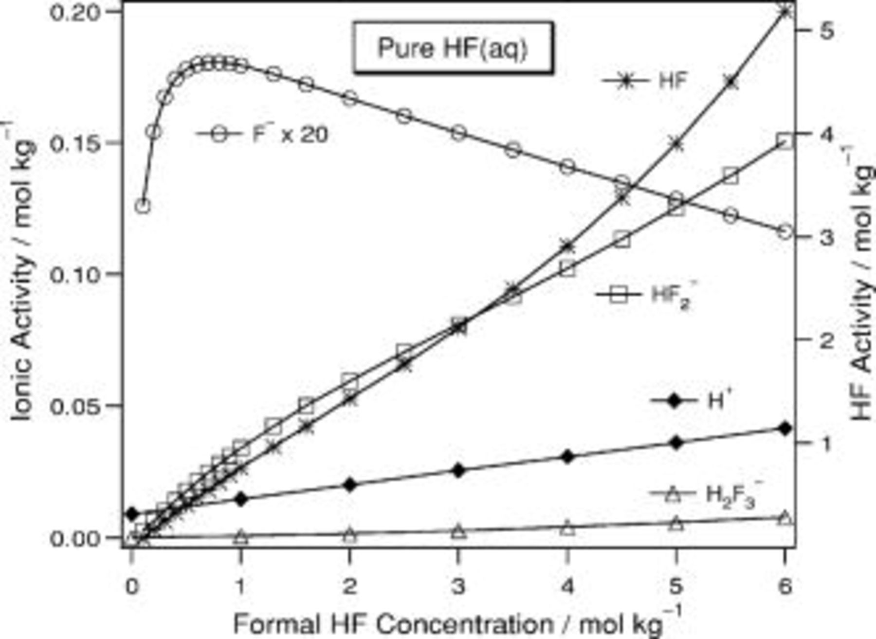
Figure 5. Predicted composition for  HF(aq).
To determine the contributions of different species unambiguously, as has been done for por-Si formation in fluoride solutions,17 one needs a set of solutions in which the activities of different species exhibit different slopes, the activity ratios of the species change greatly, and the activities vary nonmonotonically. An examination of the set of solutions depicted in Fig. 5, 6, 7, 8, 9 and 10 shows that these conditions can easily be met. In 
 (Fig. 6), the
  activity is nearly constant but
  varies from
  and
and  decreases monotonically from 1500 to 56. This behavior is much different than the previous solution.
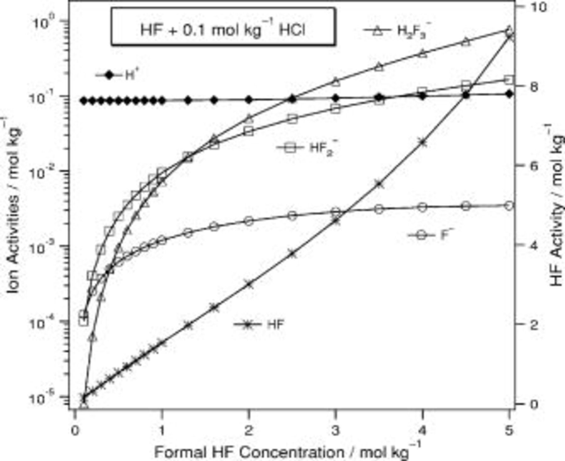
Figure 6. Predicted composition for  .
.
In  (Fig. 7),
  does not vary monotonically and
  varies from 11 to
  while
while  increases monotonically from 0.6 to 28. The activity of
  increases strongly. In
 (Fig. 8) and
 (Fig. 9), the
  activity is again rather constant.
  changes slowly and maintains a value around 1 in both solutions while
  decreases from
  to
to  . This behavior contrasts sharply with that of
  (Fig. 10), in which
  increases by almost five orders of magnitude,
  and
and  both vary nonmonotonically,
  decreases dramatically from 33 to
  , and
, and  increases from 0.3 to 83.
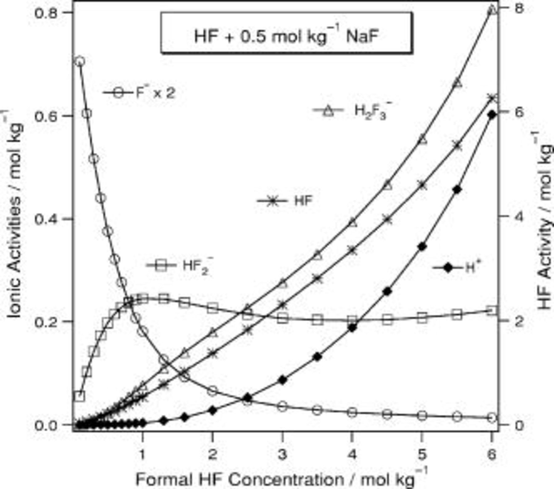
Figure 7. Predicted composition for  .
.

Figure 8. Predicted composition for 
 .
.
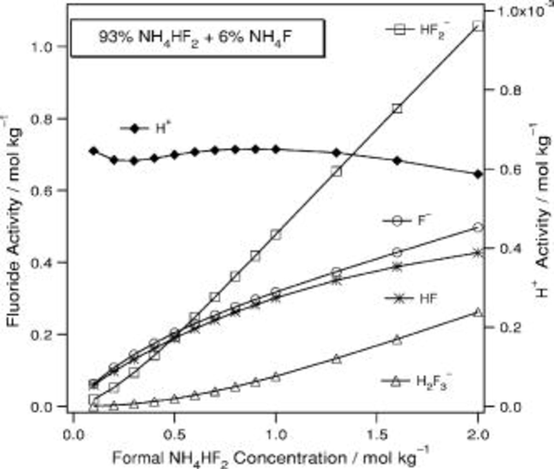
Figure 9. Predicted composition for 
 .
.
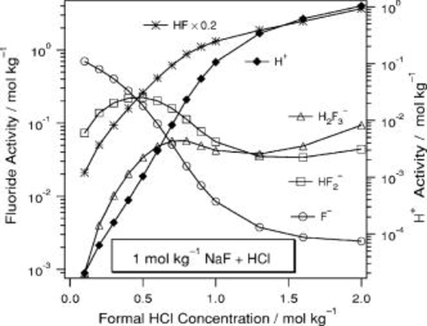
Figure 10. Predicted composition for  .
.
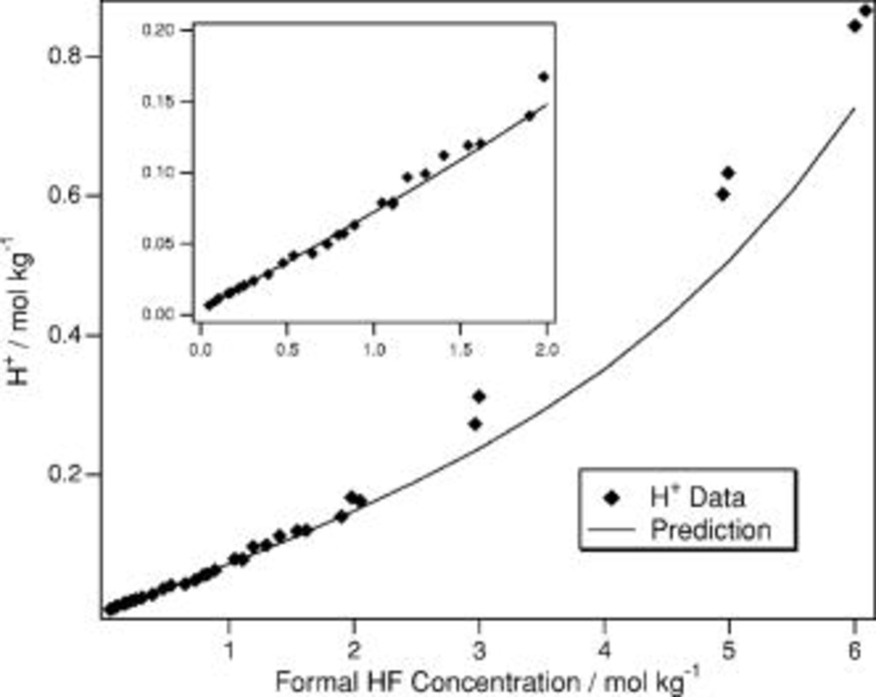
Figure 2. The predicted  molality (solid line) is compared to the
  molality (◆) as measured in Ref. 24.
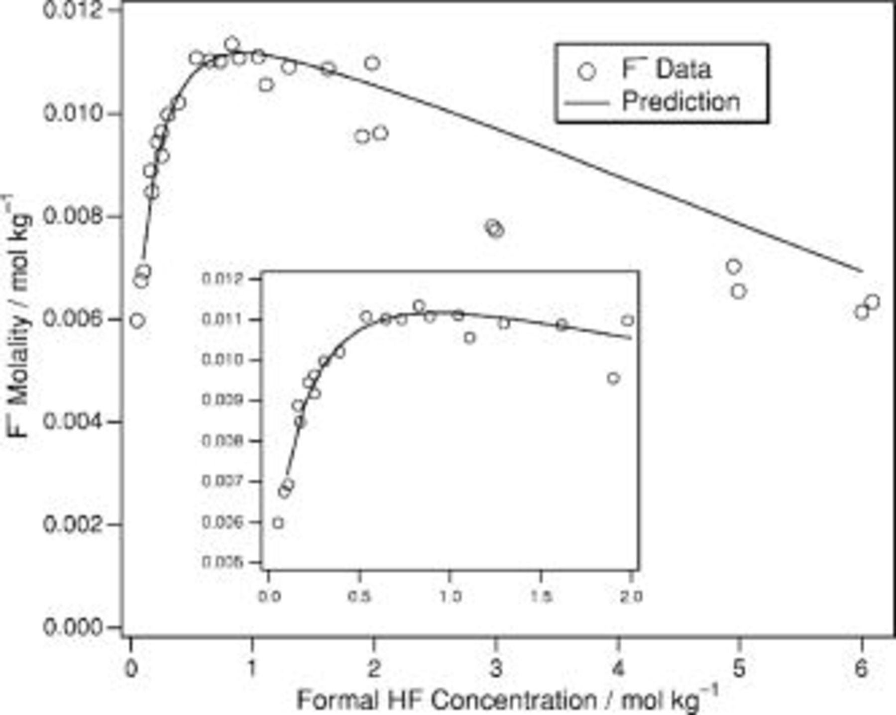
Figure 3. The predicted  molality (solid line) is compared to the
  molality (○) as measured in Ref. 24.
When choosing solutions for the study of silicon etching, it may also be important to consider other criterion.  easily precipitates out of solution and can interfere with etching as was shown, for example, in Ref. 46. The use of
  or
or  , the hexafluorosilicates of which are much more soluble, can lead to solutions of similar fluoride composition without the interference of precipitation.
Conclusions
Below  , equilibria 1, 2 suffice to describe solutions of HF. Above this, it becomes increasingly important to take equilibrium 3 into consideration. This also holds true for solutions made of, e.g.,
  or
or  . For HF solutions between 0 and
  , the use of the three equilibrium constants recommended here provides an accurate description of solution composition. Above
  , interferences such as ion-ion interactions and/or other equilibria make calculations less reliable but still useful up to
  . Applicable concentration ranges for solutions other than those containing just HF can be found in Fig. 6, 7, 8, 9 and 10.
An additional complication is the nonideality of fluoride solutions. The activity coefficients of all components differ significantly from unity at  and vary nonmonotonically with increasing concentration. The coupling of nonideal solutions with multiple equilibria means that only cumbersome numerical calculations of solution composition lead to accurate values and that estimates based on concentrations using only equilibria 1, 2 produce grossly inaccurate solution compositions.
To address this problem, numerical calculations were performed on over 150 different solution compositions to determine the concentration ranges over which good estimates of activities can be made. Furthermore, the dependence of activity on composition for each individual species was fit to an analytical expression. These expressions can be used to provide estimates of solution species activities with a minimum of effort. The activities provided by these expressions are much more accurate than common estimates derived from analytical approximations to the coupled equilibrium problem, particularly in the range of roughly  .
.
The University of Virginia assisted in meeting the publication costs of this article.