
Abstract
A new paradigm established for the investigation of errors in frequency-domain measurements was applied to the phase sensitive detection (PSD) algorithm used in lock-in amplifiers, one of two techniques commonly used for spectroscopy measurements. For additive errors in time-domain signals, the errors in the phase angle and magnitude were found to be uncorrelated, even when time-domain errors were not normally distributed. In contrast to results obtained using the frequency response analysis algorithm, errors in the real and imaginary impedance were found to be correlated, and the variances of the real and imaginary parts of the complex impedance were not equal, except at a phase angle of −π/4. A propagation of error model was established to explain and confirm the calculated statistical properties. The statistical characteristics of the results were in good agreement with experimental observations. © 2003 The Electrochemical Society. All rights reserved.
Export citation and abstract BibTeX RIS
A quantitative assessment of the error structure of impedance and other frequency-domain measurements is needed for interpretation of data in terms of physical parameters.1 2 3 4 5 6 7 8 9 A summary of the stochastic error-structure models and approaches for assessment of the stochastic error structure proposed in the literature is presented by Carson et al.10 In spite of considerable experimental and theoretical effort, the nature of the stochastic errors and the influence of instrumentation on the statistical properties of the errors has not been unambiguously established.11
Carson et al.10 have presented a new approach to address the extent to which observed statistical properties of impedance data are in fact intrinsic properties of transfer-function measurements. Simulations were used to explore the manner in which stochastic errors in time-domain signals propagated through frequency response analysis (FRA) instrumentation to the frequency domain. The approach presented was intended to serve as a paradigm for analyzing the propagation of error for arbitrary instruments and for arbitrary electrochemical cells.
The principal results were that, for propagation of additive time-domain errors through the FRA algorithm, errors in the real and imaginary impedance were uncorrelated and the variances of the real and imaginary parts of the complex impedance were equal. Interestingly, the errors in phase angle and magnitude were also uncorrelated. The observation that the FRA algorithm did not introduce correlation in the measurement suggests that the observed statistical properties may be intrinsic properties of transfer-function measurements.
The propagation-of-noise analysis presented by Carson et al. for frequency-response analysis10 is extended here to phase-sensitive detection (PSD), one of the two dominant techniques in the field. While the complex quantity simulated in this work is electrical impedance, the approach is general and applies to the measurement of other material properties such as the complex dielectric function, the complex viscosity, and acoustic impedance.
Phase-Sensitive Detection
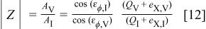
A lock-in amplifier uses phase-sensitive detection, in conjunction with a potentiostat, to measure the complex impedance.12 13 14 15 The algorithm is fundamentally different from that of the frequency-response analyzer (FRA). The FRA performs an assessment of the Fourier coefficients of the input and output signals; whereas, the lock-in amplifier measures the amplitudes of the two signals and the phase angle of each signal with respect to a reference. Thus, the impedance is measured in polar, rather than Cartesian, form. Note that modern instrumentation may employ different variations of the simplified algorithm described below.16
A reference square wave of unity amplitude was generated at the same frequency as the sinusoidal signal
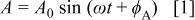
to be analyzed. The square wave can be represented by the Fourier series
where  is the phase angle of the reference signal. The measured and reference signals are multiplied, resulting in

Using trigonometric identities, Eq. 3 can be rewritten as

The product of the signals can be expanded further using the trigonometric identity for the cosine of the sum of two angles and integrated over each cycle. Only the leading term of the resulting series has a non-zero value, yielding the relationship
The integral in Eq. 5 has a maximum value when the phase angle of the square wave is equal to the phase angle of the measured signal.
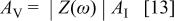
In practice, the phase angle of the generated square wave is adjusted such that the integral is maximized. The phase angle of the square wave at the maximum value of the integral yields the phase angle of the measured signal. In addition, the maximum value of the integral can be used to determine the amplitude of the measured signal. Finally, the magnitude of the impedance can be obtained from the ratio of the voltage amplitude to the current amplitude, and the corresponding phase angle can be obtained as the difference between the phase angles of the output and input signals.
Simulation of Impedance Systems
Code was written in the LabVIEW® G Language to simulate impedance measurements. Bode quadrature, which is an order  algorithm, was employed for signal integration.17 The electrochemical cell was assumed to be a single Voigt element consisting of a leading 1 Ω resistor
  in series with a parallel combination of a resistor R and a capacitor C. The value of
  was allowed to vary between 1 and
  and the capacitance C was adjusted such that the
  time constant was always
  s.
s.
The integral of the product of the test signal (input or response) and reference square wave was calculated for 16 evenly spaced values of square-wave phase angles. The spacing was refined until the 16 values of phase angle were centered around the phase angle at which the maximum value of the integrals occurred, with a spacing close to 2π/1024, the limit of the resolution. Once this level was reached, the discrete values of the magnitude of the integral as a function of phase angle were fit to a second order polynomial, and the phase angle at which this polynomial was maximized was determined. The process was repeated over several cycles until the standard deviation of the calculated impedance magnitude satisfied a specific autointegration criterion discussed later.
Time-domain signals
The forms of time-domain signals considered in the simulation study follow exactly those used for the FRA algorithm in a companion study,10 allowing a straight forward comparison among the results of the FRA and PSD techniques. The signal influenced by additive errors was described by

where  represents either a potential or current signal, and
  is a stochastic error added to the error-free value. Proportional errors were considered in the form

where  is a stochastic error.
Introduction of errors into the argument of the sine function posed serious problems for both the FRA algorithm considered by Carson et al.10 and for the PSD algorithm treated in the present work. Such errors in the argument of the sine can be considered to result from uncertainty in frequency or time. Use of Eq. 6 and 7 is predicated on the assumption that errors in measurement of frequency or time are sufficiently small that they can be neglected. A more complete description of time-domain errors is presented by Carson et al.10
Simulation of measurement techniques
The simulation method followed that presented by Carson et al.10 and is summarized as follows:
1. Noise was added to the input signal, following Eq. 6 or 7, yielding the input current 
2. The Fourier transform (FT) of the input signal was calculated and a time-domain response signal was obtained as

namely, the real inverse Fourier transform (IFT) of the FT of the product of the perturbation signal and the impedance transfer function  of the model cell. Note that
  contains noise that has been transformed through the cell's impedance transfer function. The effective digital sample rate,
  provided an upper frequency limit on the FT of the sampled signal.
3. Noise was added to the response signal, following Eq. 6 or 7, yielding the output potential  The noise distributions used were independent. Note that
  contained both transformed autocorrelated noise and added noise.
4. The impedance spectra were calculated for the FRA and PSD algorithms.
The calculations were repeated over a number of cycles sufficient to allow the autointegration criterion to be achieved. After three cycles of measurement were completed, convergence was considered to be achieved when the ratio of the standard deviation of the estimation of the magnitude to the magnitude over all cycles on the selected channel was less than 0.01. The impedance was taken to be the mean of the impedance values calculated at all cycles for the given frequency. Details on the calculation procedure are presented elsewhere.10 18
Results
Four cases were considered in the present study. Noise-free signals were first treated to verify that the algorithms yielded the expected theoretical results. Three time-domain signals, corrupted by noise, were then considered as described by Eq. 6 and 7, including normally distributed additive errors, skewed additive errors, and proportional errors. The following discussion emphasizes the results obtained for normally distributed additive time-domain stochastic errors. A brief comparison is then made to the results obtained for the skewed additive and proportional errors.
A set of 500 calculations were performed for different cell impedance values to explore the distribution of impedance errors realized in the frequency domain. The results were used to assess the dependence of the standard deviation on frequency and cell impedance, to assess the accuracy of the PSD algorithm, to test the validity of the assumption that errors in the measured impedance are normally distributed, and to identify statistical relationships among impedance components.
Error in phase angle and magnitude
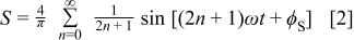
The mean error in the phase angle obtained via PSD for different cell resistance ratios  is presented in Fig. 1a as a function of frequency with
  as a parameter. The error in assessment of the phase angle was smaller than 0.003 radians (0.17 degrees). The corresponding error in the magnitude is shown in Fig. 1b. A bias error of about −0.1% was evident for the larger cell impedance values at high frequency.
Figure 1. Error in the evaluation of phase angle and magnitude as a function of frequency with  as a parameter: (a, top) phase angle and (b, bottom) magnitude.
As shown in Fig. 2, a normal distribution was seen at a frequency of 1.259 kHz where Fig. 1b reveals a small bias error in the evaluation of the magnitude of the impedance for  The standard deviation for the phase angle σϕ was 0.013 radians (0.74 degrees), and the standard deviation for the magnitude
  was 0.49 Ω, representing 0.14% of the magnitude.
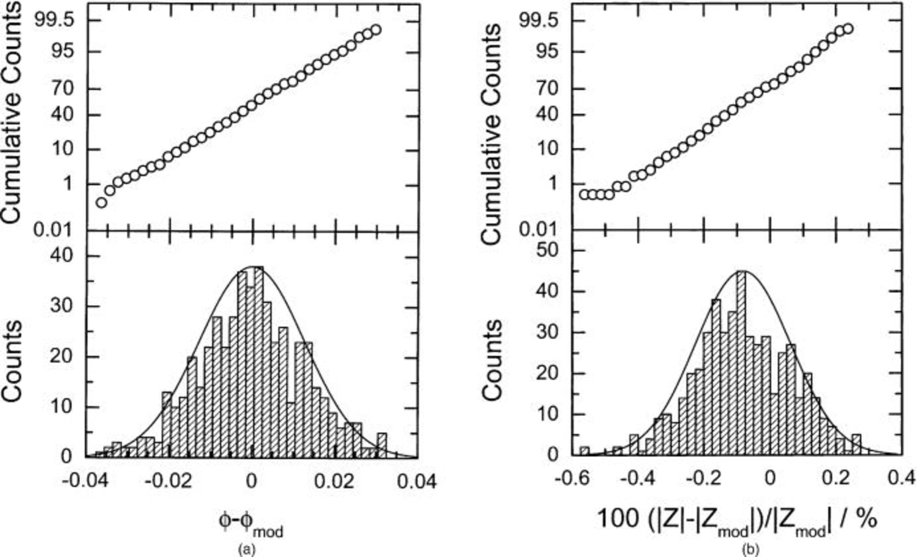
Figure 2. Distribution of calculated impedance errors obtained via PSD at a frequency of 1.259 kHz for  as a function of the normalized difference between the calculated and the model value for the impedance of the cell: (a, left) phase angle and (b, right) magnitude. The sample size was 500.
The accuracy of the individual calculations of the PSD algorithm can be assessed by examining the propagation of errors through the corresponding equations. Consider  to be the evaluation of the PSD integral in Eq. 5 for the time-domain potential signal, i.e.
where  is the amplitude of the signal and
  is the integration error. If
  is considered to be the stochastic error in the phase angle measurement, the observed value of the potential signal amplitude will be given by
The observed value of the current signal amplitude will be given by
The magnitude of the impedance is given by
The relationships among measured signals can be expressed as functions of the cell impedance as

and
Under the assumptions that the integration errors  and
and  are proportional to the respective signal amplitudes as
  and
and 
The phase angle is given by the difference
Thus
Under the assumption that the variance of phase angle for the current and potential signals are equal
Detailed Monte Carlo simulations showed that the errors in magnitude obtained from Eq. 16 were normally distributed, in spite of the presence of the cos(ɛ) term in Eq. 10 and 11 which skew the distribution for the magnitude of the individual signals. The observed value for the variance of the magnitude at a frequency of 1.259 kHz could be obtained with the variance of phase angle given by Eq. 19 and a standard deviation of the integration errors  corresponding to
  and
and  being roughly 0.06% of the magnitude of respective time domain signals. A smaller error was evident at other frequencies.
Thus, the PSD algorithm employed in the present work yielded very small errors in the evaluation of integrals  and
and  (see, for example, Eq. 9). The standard deviation of the phase angle corresponded to 1.9% of the phase angle value at a frequency of 1.259 kHz.
Dependence of standard deviation on frequency and cell impedance
The real and imaginary components of the impedance can be obtained from the relationships
and
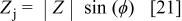
where  and ϕ are determined via PSD. The standard deviations of the real and imaginary components of the impedance obtained from the PSD simulation are presented in Fig. 3 as a function of frequency with
  as a parameter. The propagation of errors from time to frequency domain is seen to yield results that are strongly heteroskedastic, i.e., the standard deviations are strong functions of frequency, particularly as
  becomes large. Close inspection of Fig. 3, along with the more highly resolved companion Fig. 10a to be introduced later in the paper, show that for all values of the
  ratio, the standard deviation of the real part of the impedance is not equal to that of the imaginary part of the impedance, in strong contrast to the results for the FRA algorithm reported in Fig. 4 of Carson et al.10
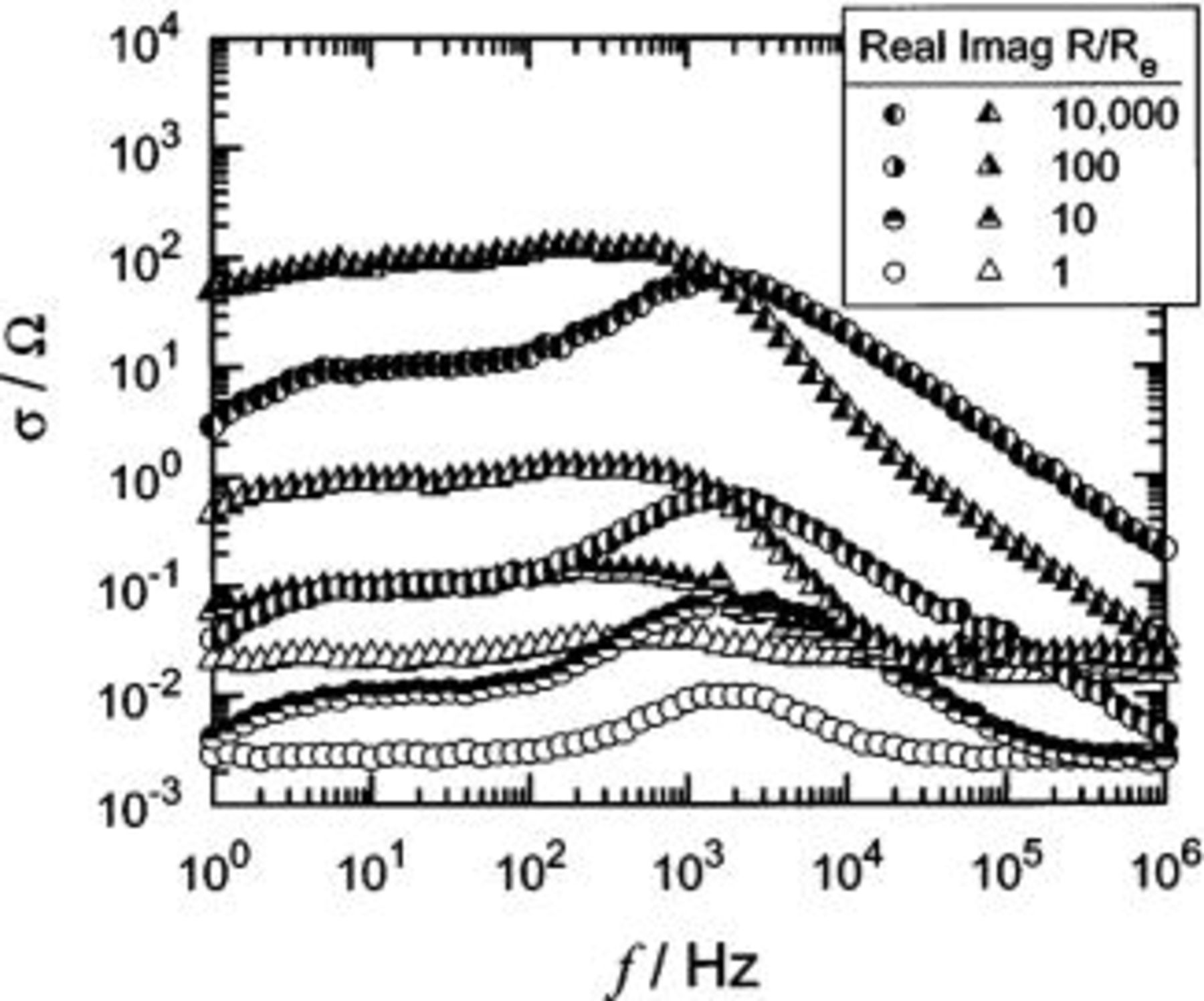
Figure 3. Standard deviation of the calculated impedance obtained using the PSD algorithm as a function of frequency with  as a parameter.
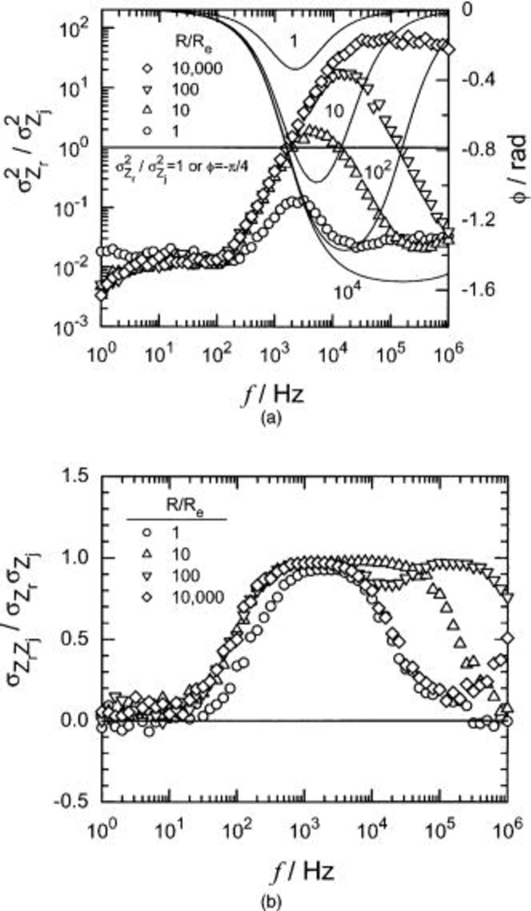
Figure 10. Calculated value of statistical parameters obtained from the PSD simulations as a function of frequency and with  as parameter: (a, top) the calculated ratio of variance for real and imaginary parts of the impedance distribution. The solid lines provide the model phase angle as a function of frequency with
  as a parameter and (b, bottom) the covariance
  Symbols are as presented in Fig. 3. The sample size was 500.
The standard deviations reported in Fig. 3 were normalized by the magnitude of the impedance and expressed in Fig. 4 as a percentage, with  as a parameter. As seen in Fig. 4, the frequency dependence of the standard deviation was, to a first approximation, proportional to the modulus
  of the impedance. The results shown in Fig. 4, therefore, support the use of modulus weighting as a preliminary strategy in regression of impedance data obtained by the PSD algorithm. The magnitude of the error observed at low frequencies is significantly smaller for the real part of the impedance than for the imaginary part. The converse is seen at high frequencies for large values of

Error in impedance simulation
The percent error in the evaluation of real and imaginary parts of the impedance is presented in Fig. 5 as a function of frequency with  as a parameter. The bias errors were largest for the imaginary part of the impedance at high frequency, but the errors were always less than 0.3% of the magnitude of the impedance. The observation in Fig. 5 of a very small bias error for the PSD algorithm contradicts and corrects the observation of a much larger bias error by Carson et al. in a preliminary report.19 While the error bound of 0.3% for the PSD is larger than the 0.07% bound reported by Carson et al.10 for the FRA, both algorithms provided a good assessment of the cell impedance.
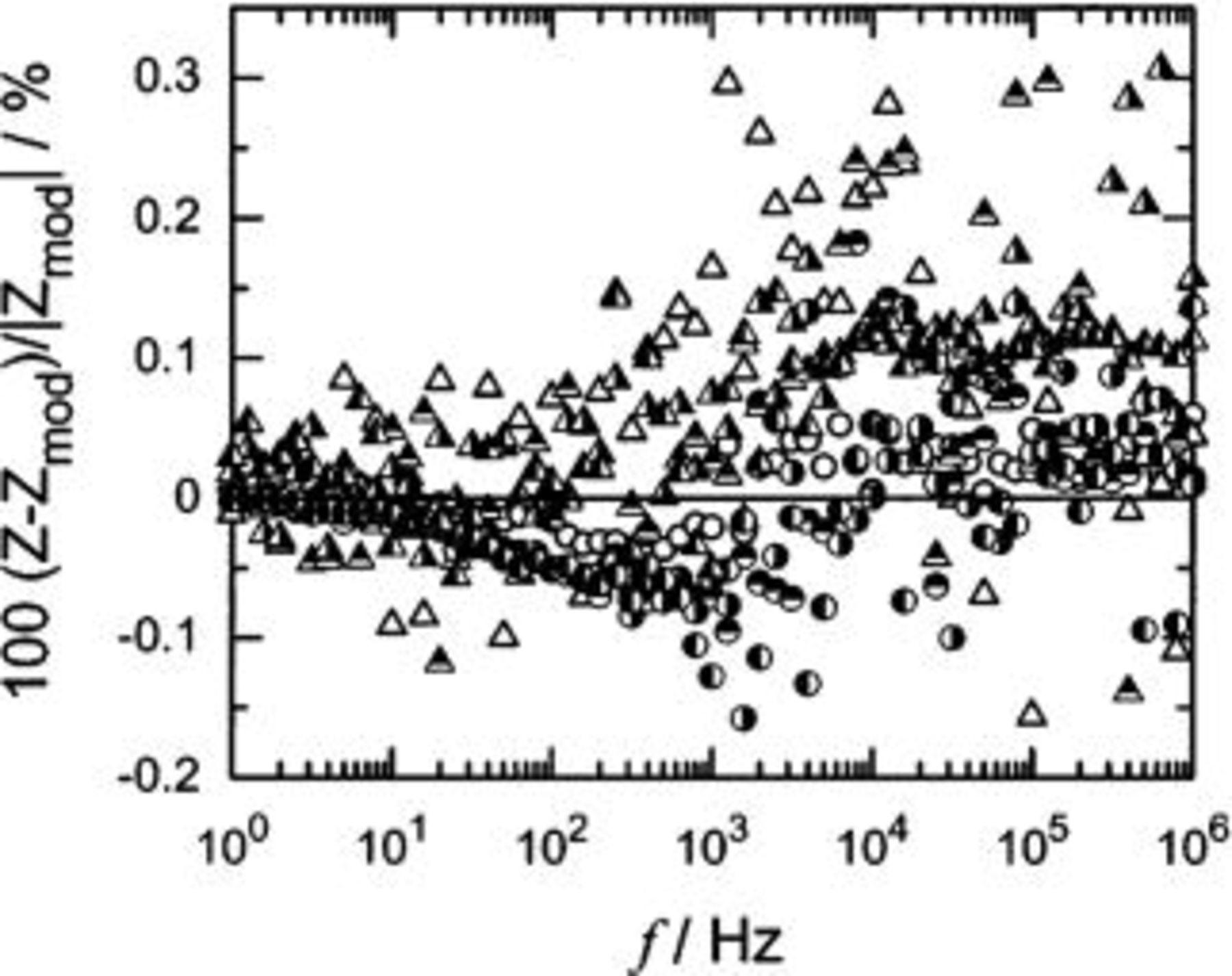
Figure 5. Percent error in the evaluation of real and imaginary parts of the impedance as a function of frequency with  as a parameter. The symbols are as given in Fig. 3.
Distribution of impedance errors
The PSD simulations generated significant numbers of outliers. The kurtosis  is presented in Fig. 6a as a function of frequency with
  as a parameter. The kurtosis has an expected value of zero for a normal distribution, but the PSD algorithm nevertheless produced large values at some frequencies. The logarithmic scale shown in Fig. 6b reveals that the magnitude of the kurtosis was generally larger than that expected for a normal distribution.
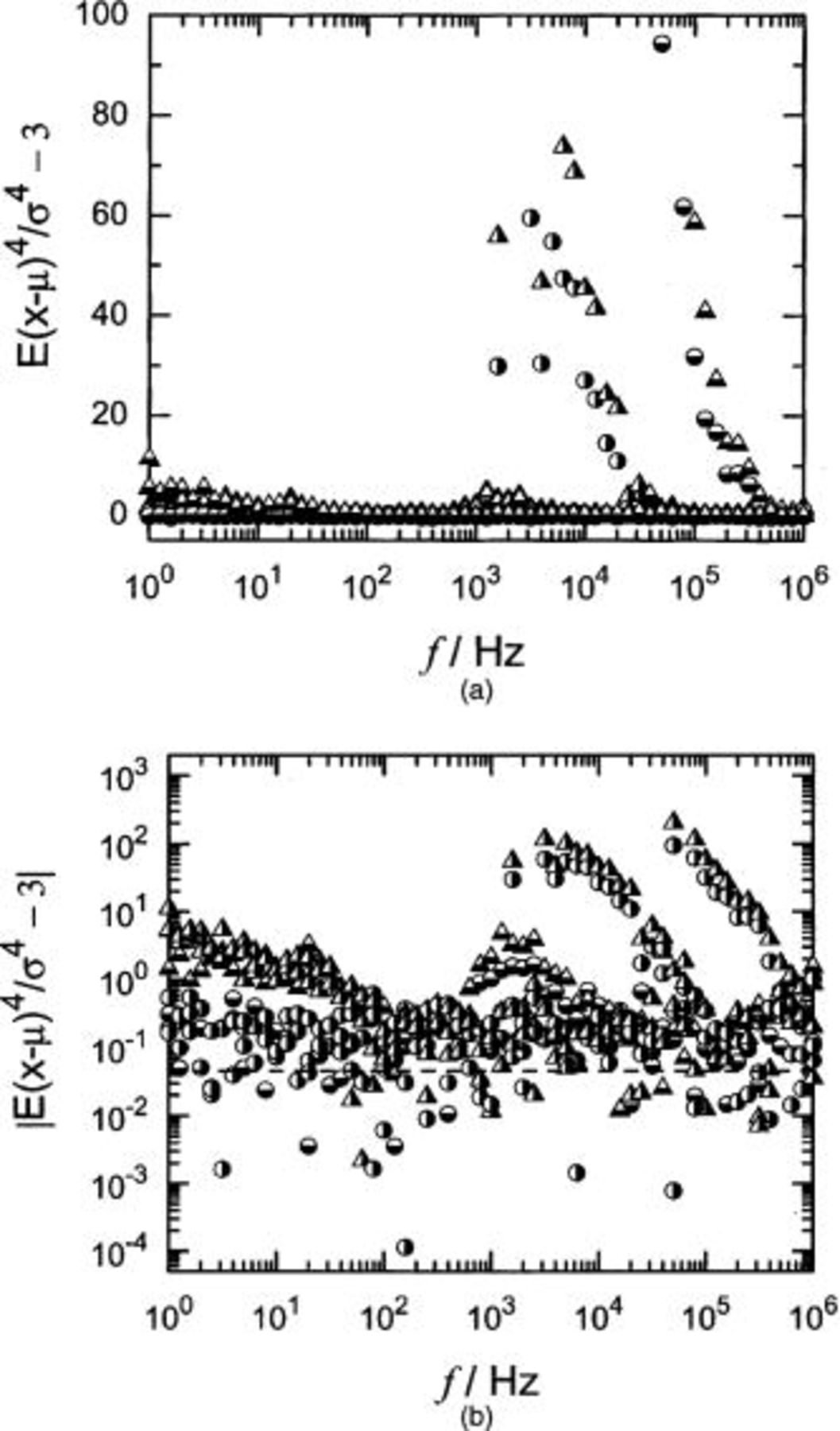
Figure 6. Kurtosis of the distributions of real (○) and imaginary (▵) parts of the impedance as a function of frequency with  as a parameter. The symbols are as given in Fig. 3. (a, top) Results presented on a linear scale and (b, bottom) absolute value of results presented on a logarithmic scale. The dashed line provides the 95.4% (2σ) confidence limit obtained for a normal random distribution.
As an example of a simulation with a large kurtosis, the distribution of impedance values at a frequency of 1 Hz is given in Fig. 7 for real and imaginary parts of the impedance at a frequency of 1 Hz for a cell impedance characterized by  The lower plot in Fig. 7a provides the histogram and the upper plot in Fig. 7a provides the estimated cumulative distribution function (i.e., a probability plot) for the random variable 100
  featured in the abscissa. The ordinate of the histogram shows the number of counts, defined as the number of realizations of the random variable that occur within a given bin. The data in the upper plot of Fig. 7a were obtained by summing the counts of successive bins and carrying out a straightforward normalization to yield probability estimates in the range of 0 to 100%. A most important feature of the cumulative-counts plot in Fig. 7a is that the scale of the ordinate is chosen such that a normally distributed random variable would yield a straight line. Therefore, a cumulative-counts plot that follows a straight line provides an indication that the distribution can be considered to be normal. A second indication of the normality of the distribution is provided by the bell-shaped curve superimposed on the histogram, which is a normal distribution with a mean and a variance equal to the sample mean and sample variance of the data. Figure 7b was constructed analogously.
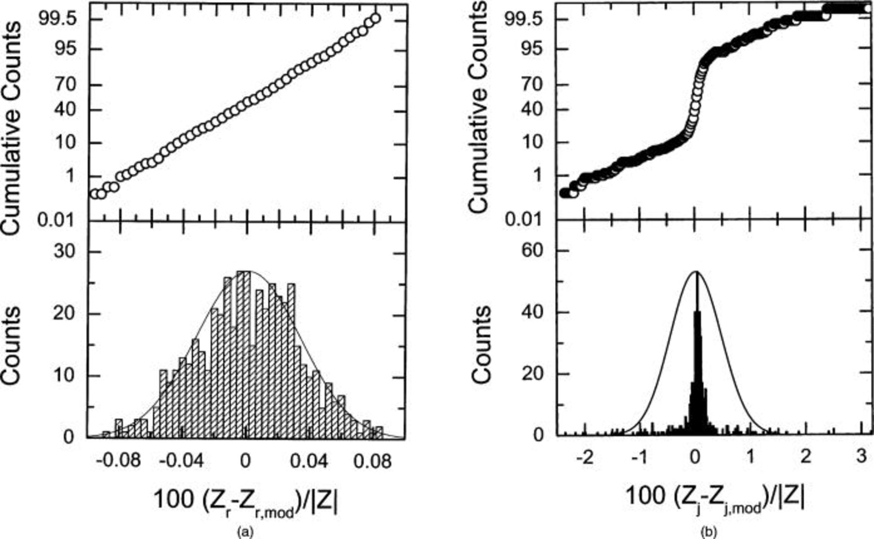
Figure 7. Distribution of calculated impedance errors obtained at a frequency of 1 Hz for  as a function of the normalized difference between the calculated and the model value for the impedance of the cell: (a, left) real part and (b, right) imaginary part. The sample size was 500.
The straight line in the cumulative probability plot indicates that the distribution can be considered to be normal for the real part of the impedance (Fig. 7a), but the presence of outliers causes the distribution for the imaginary part of the impedance to be distinctly non-Gaussian (Fig. 7b). As shown in Fig. 6b, the kurtosis for the imaginary part of the impedance at  Hz has a value of 11.3; whereas, the kurtosis of the real part of the impedance has a value of −0.19.
An explanation for the non-normal distribution shown in Fig. 7b can be found by examination of the distribution of errors in phase angle and magnitude at the same frequency. As shown in Fig. 8, the magnitude is normally distributed, whereas, the phase angle shows the same type of outliers seen in the imaginary part of the impedance. At frequencies where the phase angle is normally distributed, such as shown in Fig. 2 for a frequency of 1.259 kHz, the corresponding errors in real and imaginary impedance components were normally distributed.
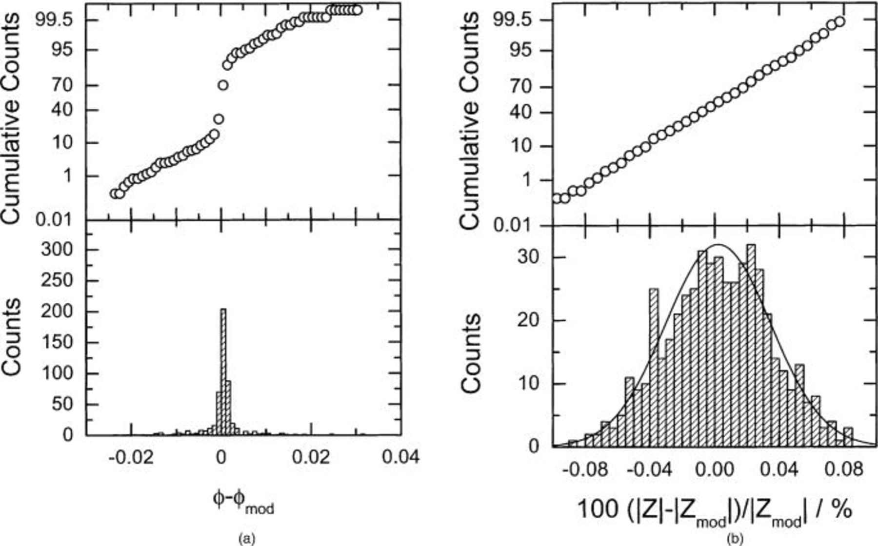
Figure 8. Distribution of calculated impedance errors obtained at a frequency of 1 Hz for  as a function of the normalized difference between the calculated and the model value for the impedance of the cell: (a, left) phase angle and (b, right) magnitude. The sample size was 500.
The presence of outliers in the real and imaginary impedance can be attributed solely to the presence of outliers in the estimation of the phase angle. The kurtosis of the magnitude of the impedance for  for example, had a mean value of
  which is comparable to the value
  obtained for a normal distribution of the same sample size, as previously mentioned. For the case described in Fig. 8, the kurtosis for the phase angle at
  Hz had a value of 11.3; whereas the kurtosis of the magnitude of the impedance had a value of −0.19.
As seen in Fig. 6b, the distribution for the real part of the impedance was much more sensitive to outliers in the phase angle at intermediate frequencies. An explanation is found from a Taylor series expansion about the expected values for ϕ and  i.e.
i.e.

and

where E {ϕ} refers to the expectation of ϕ, and the braces not preceded by an expectation operator denote the evaluation of a function at the expected values of ϕ and  The outliers in ϕ, represented by the term
  in Eq. 22 and 23, have a lesser impact on the evaluation of the real part of the impedance at frequencies where sin ϕ tends toward zero. At
  Hz, the distribution of errors in
  is driven by the distribution of the magnitude errors
  whereas the distribution of errors in
  is driven by the distribution of the phase angle errors
  At intermediate frequencies, both the phase angle and magnitude errors contribute simultaneously to the errors realized in the real and imaginary components of the impedance.
Statistical relationships among impedance components
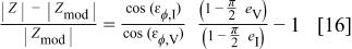
As shown in Fig. 3, the variances of real and imaginary parts of the PSD-determined impedance are not equal. A propagation of error analysis, beginning with Eq. 20 and 21 and following Eq. 22 and 23, yields

and

for the variance of the real and imaginary parts of the impedance, respectively. The covariance can be expressed as

Equation 24, 25, and 26 describe how the variances and covariance of the phase angle and magnitude variables realized in a PSD measurement affect the variances and covariance of real and imaginary components of the impedance.
From Eq. 24
25
26 it can be readily concluded that the necessary and sufficient condition for  is that

and the necessary and sufficient condition for  is that

It is worth noting that the conditions 27 and 28 involve five variables. Three of these, namely 
 and
and  are PSD measurement characteristics, and the remaining two,
  and ϕ(ω), are functions of the cell impedance and are therefore explicit functions of frequency. Under the assumption that errors in phase angle and magnitude are uncorrelated, a necessary and sufficient condition which allows equation 27 and 28 to be satisfied for any cell impedance (i.e., all frequencies) is that
  for all frequencies.
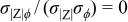
The calculated value of the covariance  is presented in Fig. 9a in the correlation coefficient form
  as a function of frequency. The correlation coefficient is centered about zero, indicating that
  and ϕ is uncorrelated. Hence,
  was effectively equal to zero for all frequencies.
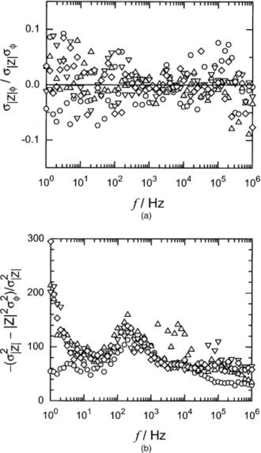
Figure 9. Calculated value of statistical parameters obtained from the PSD simulations as a function of frequency and with  as parameter: (a, top) the correlation coefficient
  and (b, bottom) the difference
  The sample size was 500.
The difference  as shown in Fig. 9b, was always less than zero. The value of
  scaled by the variance of the magnitude, i.e.,
  had values ranging between 50 and 300 for all cell impedances evaluated. As
  was not equal to zero at any frequency, the conditions 27 and 28 could be satisfied only at specific values of cell impedance. The PSD simulation studies showed that the variances for real and imaginary parts of the impedance are equal for
  and the covariance for real and imaginary parts of the impedance are equal to zero only for
The ratio of the real and imaginary variances is given in Fig. 10a as a function of frequency with cell impedance  as a parameter. The solid lines provide the model phase angle as a function of frequency. The ratio
  is equal to unity only under conditions such that the cell impedance is equal to −π/4. As shown in Fig. 10b, the covariance
  tends toward zero at low frequencies where the phase angle tends toward zero.
These observations are consistent with the necessary and sufficient conditions 27 and 28. First, since Fig. 9a suggests that  for all frequencies, Eq. 27 reduces to
  which is always satisfied at
  Hence, since Eq. 27 is always satisfied, it follows that
  for all frequencies where the phase angle is equal to ±π/4. Second, given that
  and that
  when
when  it follows that Eq. 28 is satisfied when the phase angle is equal to zero. Hence, it follows that
  tends toward zero at all frequencies where the phase angle tends toward zero. This reasoning is based on the observation that
  however, the zero-value conjecture must be tested within the rigorous statistical framework that is presented next.
Hypothesis Testing
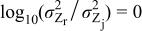
The Student's t-test statistical analysis of several conjectures of the form  at a significance level of
  is presented in Table I for normally distributed errors in the time-domain signals. In Table I
  represents the mean observed value, which should be compared to the hypothesized test value of 0,
  represents the standard deviation of the observed value,
  is the probability of observing the given sample result under the assumption that the null hypothesis is true, and
  is a test for rejection of the null hypothesis. If
  or
or  the null hypothesis can be rejected, and it can be concluded that x is statistically indistinguishable from zero.
Table I.
Student's  -test statistical analysis of the conjecture -test statistical analysis of the conjecture  at a significance level of at a significance level of  for normally distributed errors in the time-domain signals. for normally distributed errors in the time-domain signals. | ||||||
|---|---|---|---|---|---|---|
| Test |
 |
 |
 |
 |
 |
 |
| 1. |
 | 1 | −1.57 | 0.28 |
 | 21.9 |
| 10 | −1.27 | 0.81 |
 | 6.2 | ||
 | −0.75 | 1.2 |
 | 2.4 | ||
 | 0.20 | 1.7 | 0.34 | 0.48 | ||
| 2. |
 | 1 | 0.34 | 0.36 |
 | 3.7 |
| 10 | 0.56 | 0.39 |
 | 5.6 | ||
 | 0.64 | 0.37 |
 | 6.7 | ||
 | 0.46 | 0.35 |
 | 5.1 | ||
| 3. |
 | 1 | −0.011 | 0.052 | 0.12 | 0.79 |
| 10 | −0.0032 | 0.053 | 0.63 | 0.24 | ||
 | 0.0089 | 0.054 | 0.21 | 0.64 | ||
 | 0.0033 | 0.040 | 0.53 | 0.32 | ||
| 4. |
 | 1 | −65 | 25 |
 | 10.1 |
| 10 | −97 | 37 |
 | 10.2 | ||
 | −90 | 34 |
 | 10.5 | ||
 | −88 | 39 |
 | 8.9 | ||
It should be noted that the Student's t-test can be applied for sampling from normal random distributions. Application of t-test statistics to a sample set consisting of all frequencies, therefore, can have meaning only for cases where no trending is seen as a function of frequency. The results presented in Fig. 9 and 10 indicate that the t-test statistic has meaning for test 3 (i.e., for the hypothesis  , but are not as meaningful for the other tests reported in Table I. The statistical results reported for the other tests provide a contrast with the results reported by Carson et al.10 for the FRA calculations.
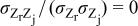
The Student's t-test shown as test 1 in Table I indicates that the sample mean value observed for  was not equal to zero. In addition, the real and imaginary components of the impedance were correlated, i.e.,
  Test 3 indicates that the modulus and phase angle calculated from the impedance components were uncorrelated, i.e.,
  Test 4 demonstrates that the expression
  was not satisfied.
Similar results were obtained for the skewed time-domain error distribution. The modulus and phase angle calculated from the impedance components were uncorrelated, but the variances for real and imaginary parts of the impedance were not equal, the real and imaginary components of the impedance were correlated, and the expression  was not satisfied.
The magnitude and phase angle were correlated when proportional time-domain errors were introduced.
Comparison to Experiments
It should be noted that the present simulation was based on the assumption of idealized instrumentation, and that actual instrumentation introduces errors such as those associated with nonoptimal selection of current measurement circuitry that are not simulated here. Thus, it cannot be expected that the simulations presented here would provide exact predictions of experimental observations. Nevertheless, general observations have been made that merit comparison with experimental data reported in the literature.
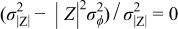
In 1984, Zoltowski reported the results of a series of replicated measurements used to assess the error structure of impedance measurements.1 His intention was to rationalize use of modulus weighting, which implies that the variances for real and imaginary components are equal. The experiments were performed using a potentiostat and a phase-sensitive device for a five-element  ladder circuit. At least 30 replicated measurements were obtained at each of four frequencies. The results are presented in Fig. 11 in the form of the ratio of the variance for real and imaginary components of the impedance. The ratio has a value less than unity at higher frequencies and has a value greater than unity at the lowest frequency measured. The corresponding phase angle is also given in Fig. 11 to show that the phase angle has a value of −π/4 between the frequencies where the ratio changes from being greater than unity to being less than unity.
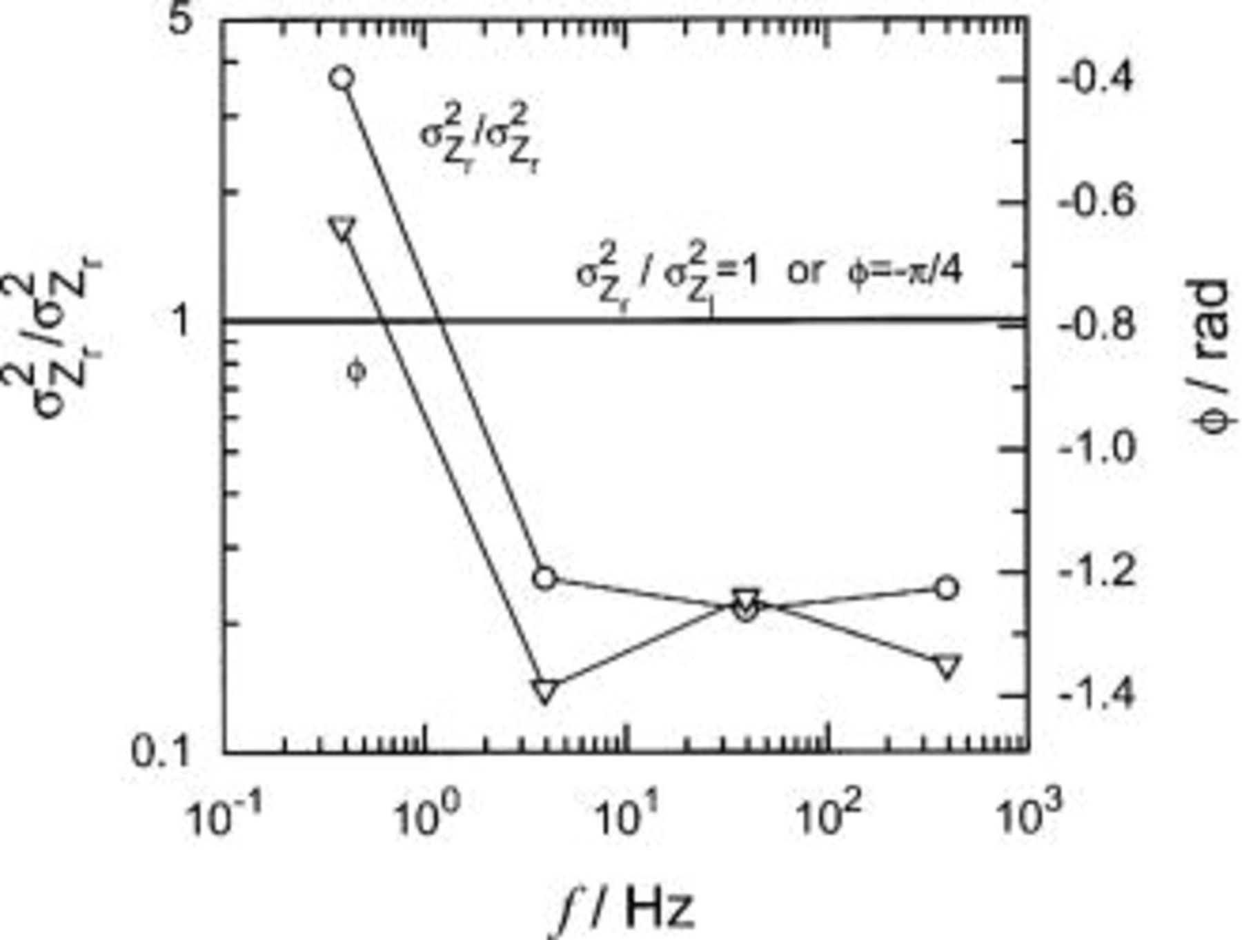
Figure 11. Ratio of the variance of the real and imaginary parts of the impedance obtained using phase-sensitive detection as reported by Zoltowski.1
The result that the variance for the real and imaginary parts of the impedance were not equal for the PSD calculations was also observed using a measurement model analysis of coupled FT/PSD experimental data provided by Lasia for the hydrogen evolution reaction on pressed powder electrodes.20 The experimental procedure is described by Hitz and Lasia.21 Three replicated measurements were obtained for each condition.
As shown in Fig. 12, the ratio of variances was centered about one for data collected at low frequencies using the FT, but was centered above one for data collected using the PSD. The F-test indicates that most of the ratios for PSD measurements fall within the 99% F-test confidence interval (given by horizontal lines). Thus, the F-test cannot be used to conclude that the variance of the real part of the PSD-determined impedance differed from the variance of the imaginary part. The Student's t-test, however, indicated that the mean value of the quantity  obtained for the PSD portion of the measurements was not equal to zero. The corresponding value of 0.061 for the FT portion of the measurement was statistically indistinguishable from zero.
The experimental results presented above support the conclusions of the present analysis that, in general, the variances for the real and imaginary parts of the impedance are not equal when measured by the PSD algorithm. In addition, the ratio of the variances of real and imaginary components of the impedance reported by Zoltowski,1 and presented in Fig. 11, cross from being greater than unity to being less than unity at a phase angle of −π/4, as predicted by the present work.
There is a discrepancy, however, in that the simulations predict that the variance of the real part of the impedance should be smaller than the variance of the imaginary part of the impedance for phase angles between 0 and −π/4 (and larger for  . The phase angle for the experiments shown in Fig. 12 never reached a value of −π/4; thus, the simulations presented in the present work predict that the ratio of the variances of real and imaginary components of the impedance should be less than unity for all frequencies. Instead, the ratio of the variances of real and imaginary components of the impedance was greater than unity. The same discrepancy exists with the results presented in Fig. 11.
The reason for the discrepancy probably rests in the details of the phase sensitive detection algorithm. The present simulation was conducted under galvanostatic modulation, in which the current was the input signal, and potential was the output. The analysis of the statistics of input and output signals, presented by Carson et al. ,22 showed that the PSD algorithm used reduced the apparent variance of the real part of the input signal. The simulations were conducted under galvanostatic modulation, in which current was the input signal. The experiments were conducted under potentiostatic modulation, in which potential was the input signal. The discrepancy may be attributable to differences in modulation signal, but new simulations are needed to confirm this.
As second difference rests in the manner in which the reference square-wave signal is used. The present simulation follows an algorithm in which the signals are multiplied by a single reference square wave. In the commercial instrumentation employed by Hitz and Lasia,20 21 two operations were carried out, one multiplication with a square wave followed by another with a square wave shifted by 90 degrees.16 The specifics of the phase sensitive detection algorithm will affect the error structure of the PSD analysis. In all cases, however, such algorithm-specific details can be taken into account in the context of a systematic and statistically rigorous analysis, as illustrated in the paradigm presented in this paper, to elucidate the structure of the frequency-domain errors.
Conclusions
The objective of this work was to investigate the manner in which frequency-domain errors arise from time-domain measurements through phase-sensitive instrumentation. In the present work, an idealized potentiostat that had unautocorrelated input noise was assumed, and the output noise contained an autocorrelated component due to propagation of input errors through the cell impedance.
The PSD simulations provided an accurate assessment of the impedance. For all conditions, the error in the real and imaginary impedance obtained was less than 0.3%. This error was about three times larger than the maximum error reported by Carson et al.10 for simulation involving the FRA algorithm. The impedance errors were heteroskedastic, but, remarkably, the variances of real and imaginary parts of the impedance were not equal except for the special condition where the phase angle had a value of −π/4. These results were supported by experimental observation from the literature.
The modulus and phase angle measured by the PSD algorithm were uncorrelated; however, the real and imaginary parts of the impedance values derived from these measurements were correlated. A propagation of error analysis was used to show that, if 
 represents a necessary and sufficient condition for satisfying
  and
and  at arbitrary frequencies. While the hypothesis tests indicated that the condition
  was satisfied, the PSD simulation yielded
  for all frequencies.
The results of the present simulation for PSD and those presented for FRA10 explain the differences between the statistical properties for PSD measurements reported by Zoltowski,1 in which the variances for real and imaginary parts of the impedance were not equal, and those reported for FRA measurements by Orazem and co-workers,8 23 24 25 26 in which the variances for real and imaginary parts of the impedance were equal.
The remaining question is whether either of the measurement strategies can be said to provide the intrinsic statistical properties of transfer-function measurements.11 The discussion should be limited to propagation of additive time-domain errors because assumption of proportional time-domain errors gave results that were inconsistent with experimental observations for FRA measurements. Both the PSD and the FRA techniques provided very accurate assessments of the cell impedance spectra. The principal difference between the two techniques rests in the statistical properties of the results. The FRA algorithm yielded real and imaginary components that were uncorrelated, modulus and phase angle components that were also uncorrelated, and values of  equal to zero. Thus, it can be argued that the FRA algorithm did not introduce undesired correlations. On the other hand, the PSD algorithm introduced undesirable features in the sense that the real and imaginary components were correlated and values of
  were not equal to zero. In addition, the impedance values calculated using the PSD algorithm were not normally distributed for all frequencies; whereas, the impedance values were normally distributed when calculated using the FRA algorithm. Finally, as discussed in a companion paper,22 the different statistical properties obtained with PSD simulations could be attributed in part to bias errors introduced when the square-wave reference signal was in phase with the measured signal. Thus, it can be argued that, of the two approaches, it is the FRA which provides statistical properties intrinsic to transfer-function measurements. It must be noted, however, that this statement holds only for additive time-domain errors.
In a more general sense, the frequency-domain error structure is determined by the nature of errors in the time-domain signals and by the method used to process the time-domain data into the frequency domain. The cell impedance influences the frequency-dependence of the variance of the measurements, but, with the exceptions noted for  and
and  for the PSD algorithm, the cell impedance does not influence whether the variances of real and imaginary components are equal or whether errors in the real and imaginary components are uncorrelated.
The results presented here suggest that different strategies may be appropriate for regression of models to impedance data resulting from use of PSD and FRA instrumentation. A weighting strategy based on the assumption of equal variances for real and imaginary components, such as proposed by Orazem et al. ,23 24 25 is most appropriate for data collected using FRA instrumentation. A weighting strategy employing different variance values for the real and imaginary components would be most suitable for data collected using PSD instrumentation. The form that the PSD error structure should take may follow the modified proportional error form proposed by Macdonald and co-workers,4 5 6 although experimental verification is needed.
Acknowledgments
The financial support of the Engineering Research Center for Particle Science and Technology at the University of Florida is gratefully acknowledged. The authors thank Professor A. Lasia, Department of Chemistry, University of Sherbrooke, for sharing his experimental data and for providing a helpful informal review of the manuscript, and Dr. B. Tribollet, CNRS, Paris, for a helpful informal review of the manuscript.