Modeling teams performance using deep representational learning on graphs

Abstract

Most human activities require collaborations within and across formal or informal teams. Our understanding of how the collaborative efforts spent by teams relate to their performance is still a matter of debate. Teamwork results in a highly interconnected ecosystem of potentially overlapping components where tasks are performed in interaction with team members and across other teams. To tackle this problem, we propose a graph neural network model to predict a team’s performance while identifying the drivers determining such outcome. In particular, the model is based on three architectural channels: topological, centrality, and contextual, which capture different factors potentially shaping teams’ success. We endow the model with two attention mechanisms to boost model performance and allow interpretability. A first mechanism allows pinpointing key members inside the team. A second mechanism allows us to quantify the contributions of the three driver effects in determining the outcome performance. We test model performance on various domains, outperforming most classical and neural baselines. Moreover, we include synthetic datasets designed to validate how the model disentangles the intended properties on which our model vastly outperforms baselines.

1 Introduction

What makes a team effective is a long-standing problem widely studied across disciplines and applicative contexts. Several factors such as communication, coordination, distinctive roles, interdependent tasks, shared norms, personality traits, and diversity are relevant aspects shaping team performance [1–6]. Yet, our understanding of teams as evolving systems of interacting individuals as well as the relation between team composition and performance is still partial [7–9].

When studying teams, a key issue is combining the features (e.g., skills, socio-demographic indicators, relations, and past experiences) of single individuals at the team level. Straightforward solutions are offered by the so-called compositional models [10]. They rely on the assumption that each team member’s contribution is equal. As a result, attributes of single individuals are considered additive and possibly averaged in a summary index [10]. However, this approach provides an extreme simplification of the dynamics at play. In contrast, in compilational models, team-level attributes are considered complex combinations of individual-level properties [10]. The intuition is that teams could be more than the sum of their parts. Perspectives from Complexity and Network Science offer natural frameworks to capture and investigate this direction [1–5, 11–16]. Within these approaches, teams’ performance has been linked to three effects. The first are topological effects. The internal structure of a team, emerging from the interactions of its members, plays a crucial role in determining performance [1–5, 17]. The second are centrality effects. Teams’ performance is influenced by the importance/role of a team with respect to the ecosystem to which it belongs. Indeed, collaborations (i.e., connections) with people outside the team, sharing and advertising of one’s work are key factors that might boost teams’ performances by leveraging popularity, rich get richer phenomena, and providing access to relevant as well as novel information [11–13]. Centrality effects, commonly encoded through network metrics such as degree, betweenness, and closeness [18], roughly capture the overall visibility of a team in the system as well as its ability to be part of informative flows. The third are contextual effects. The success or failure of a team can be guided by the context to which it belongs and in which it develops, regardless of how internal or external relations are structured. For example, the number of citations received by articles published by research teams might vary significantly across different disciplines [19]. It depends on the context where the activity, such as a publication, takes place.

Identifying the drivers of team performance is an important step but does not solve the problem. Indeed, the hand-design of features that allow models to capture the complex effects of such factors is far from trivial. Recent advancements in extending deep learning architectures to graph-structured data can help us solve this challenge [20–23]. Graph Neural Networks (GNNs) offer a natural way to derive high-order representations of interacting systems by inferring, in this application, the relevant and holistic features of the team as a result of a learning procedure. In this regard, the interacting systems of interest fit well in a graph-based scenario. The whole graph represents the collaborative activity’s ecosystem, and the teams are represented by their parts (i.e., subgraphs). Therefore, the task of modeling team performance can be rephrased in terms of designing graph representation learning methods able to project the subgraph structures into a higher dimensional space, called embedding space, that a downstream classifier can subsequently leverage to solve tasks of interest.

Learning methods on graphs have greatly improved in recent years [24]. However, the literature on GNNs aims at developing architectures useful in learning representations for nodes [20–22], edges [25, 26] or entire graphs [23]. Therefore, these methodologies may not be optimal in modeling the broad spectrum of teams’ (i.e., subgraphs) peculiarities. As highlighted in Alsentenzer et al. [27], subgraphs have non-trivial internal structure, border connectivity, and notions of neighborhood and position relative to the rest of the graph. Therefore, tackling the problem of subgraph embedding requires the design of architectures able to capture graph features that may not be defined for finer and coarser graph components such as nodes or whole graphs.

Here, we present a compilational model based on graph neural learning that captures the dynamics that shape team performance. The model explicitly considers for topological, centrality, and contextual effects. We summarize our contributions as follows:

• We propose MENTOR (ModEliNg Teams Performance Using Deep Representational Learning On GRaphs), a new three channels architecture (Fig. 1) that models team performance by leveraging topological, centrality and contextual effects. In more depth, this architecture features graph neural learning methods defined on subgraph structures;

  Figure 1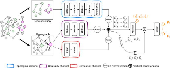

  

  MENTOR. The architecture of our model is based on the usage of three channels: topology (T), centrality (C), and contextual (L). Each channel returns a corresponding embedding vector for each subgraph $S_{i}$. The outputs of the three channels are then merged by means of an attention mechanism that estimates the importance of a specific effect

• We endow the model with two attention mechanisms that allow us to examine targeted parts of the proposed deep architecture in more detail. A first mechanism, defined at the node level, allows pinpointing key members inside the team. A second mechanism, defined at the channel aggregation level, allows us to quantify the contributions of topological, centrality, and contextual effects in determining the outcome. These two mechanisms not only enhance the model’s expressivity but also shed light on the inner workings of the proposed architecture, providing some degree of interpretability;

• We test the model’s performance on various domains. Furthermore, we introduce synthetic datasets designed to include topological, centrality, and contextual effects. This allows us to test whether the proposed architecture can learn disentangled representations of the intended properties. We then show how the proposed model outperforms most classical and neural baselines on the analyzed datasets.

2 Related work

An extensive body of research has focused on the key factors that affect team performance. Works from a range of disciplines identified features like regular communication, coordination, distinctive roles, interdependent tasks, and shared norms as the building blocks of effective teams [1–4, 28].

Several models have been proposed and evaluated in different contexts. For example, the seminal work by McGrath [29] introduced an input-process-output (IPO) model where antecedent conditions and resources (i.e., input) maintain internal processes and produce specific products (i.e., output). According to this model, the necessary antecedent conditions and the processes of maintaining teams define their effectiveness. A relevant body of literature is attributable to this paradigm and its extensions; however, it is too simplistic and unable to accurately account for all the complex interactions that influence team performance [30].

More generally, research on team composition focuses on team members’ attributes and their combination’s impact on processes, emergent states, and ultimately performance [8]. The research on the subject can be grouped into three main areas [31]: i) studies focusing on the features of team members, ii) studies focusing on how such features are measured, and iii) studies that investigate alternative approaches to team composition. As part of the last category, Kozlowski and Klein [10] described composition processes as relatively simple combination rules aimed to shift from lower-level units (i.e., individual) to higher-level constructs (i.e., team-level attributes). Two main general approaches are commonly used to describe team composition. The first category considers compositional models. As mentioned above, these assume that members are “isomorphic” and that their contribution is equally weighted. Examples are models based on mean and diversity indices. The former computes team-level scores as the mean of the individual-level attributes [32]. This is the so-called “all-stars” approach. In fact, it implies that the best teams are those formed by ensembles of top individuals. The latter, instead, assumes that the heterogeneity (i.e., diversity) of the attributes at the lower level is crucial, and it is often operationalized with measures like variance [32]. In general, compositional models are simplistic. They do not capture the dynamics at play or apply to tasks/contexts where individual contributions are less significant than teamwork. An example comes from sports, where an “all-star” team is not necessarily the best. Furthermore, empirical findings show that team performance is not a monotonic function of diversity [33]. The second category considers compilational models. The overarching assumption is that team-level attributes cannot be computed from simple statistical measures of lower-level quantities. Teamwork implies interactions between members and, thus, between their attributes. Within this vision, teams are considered complex adaptive systems of multiple parts that continually interact and adapt their behavior in response to the behavior of the other parts [34]. Thus, compilational models consider complex combinations of members’ attributes such as the relative position or status of the highest or lowest individual [8, 35] or network features that capture the structural properties of the social connections linking members between and within teams [17, 36]. By modeling such systems, researchers seek to understand how the aggregate behavior emerges from the interactions of the parts, integrating multiple levels of analysis to build a more thorough understanding [37].

From a methodological point of view, Machine Learning (ML) has been recently applied to team modeling in a wide range of applicative scenarios, mainly with cross-sectional data and hand-designed features carefully engineered by domain experts. In particular, we refer to the example of online games [38–40] where interactions and performances of teams are captured through real-time data collection platforms. Similar to the goals of this work, Chen at al. [40] aimed at understanding what makes a good team in Honor Kings, a massive online game with more than 96 million users. However, they limit their analysis by i) focusing on specific aspects while overlooking the holistic picture underpinning team dynamics ii) adopting hand-designed features that often fail to capture the complexity of high-order functional relationships. All these limitations clearly pointed out how these approaches should be refined to unravel the complex threads behind these scenarios.

Recent literature on graph representation learning shows how deep learning architectures and, hence, implicit feature engineering can be achieved by designing methods that, without hand-crafted features, capture patterns of compound interactions. In particular, these methods deal with graph-structured input data. In more depth, several network embedding frameworks were proposed to represent graph nodes as low-dimensional vectors [41–44]. Such representations aim to preserve network topology structure and node features, delivering embeddings that can be used downstream for classification, clustering, and link prediction through classical machine learning methods. In this work, we will focus on a class of models broadly referred to as graph neural networks (GNNs) [45, 46]. GNNs perform neighborhood aggregation through a procedure called neural message-passing [47], where the embeddings of nodes are obtained by recursively pooling and transforming representation vectors of their neighborhood [20–23]. Despite works such as references [48, 49], which try to outline a general unifying GNN framework for all of the applications introduced so far, deep learning on graphs is a fast-evolving field, and many theoretical results still need to be proven. A fair amount of recent research [23, 50, 51] involves shedding light on GNNs expressivity, with particular focus on understanding: (a) the relation between the depth of a GNN architecture and over smoothing [52–54], (b) the interplay of positional and structural effects [55, 56], (c) the difference between homophily and heterophily in graphs [57, 58].

Most of the introduced literature on GNNs focuses mainly on node-level or graph-level tasks [21–23]. As we will explain later, team modeling involves a subgraph learning problem. Subgraph embedding tasks using GNNs are still an underexplored area of research, with SubGNN model [27] being the most notable exception. Similar to the framework that we propose, SubGNN tackles the problem of embedding general subgraphs by specifying three channels designed to capture distinct aspects of subgraph structures. However, being SubGNN a model built disregarding domain knowledge on team performance, this architecture overlooks several of the effects outlined in Sect. 1 as we will show in Sect. 5.3. Within this view, to the best of our knowledge, our work represents the only Graph Neural Network model explicitly built to learn disentangled team representations aggregated through attention mechanisms.

3 Model

This section introduces the proposed model, MENTOR, built by leveraging and extending recent graph representation learning techniques [22, 23, 59]. The model features three main components, which are then aggregated through a soft-attention mechanism [60] that provides expressivity and some degree of interpretability. The model’s outcome aims to capture the performances reached by teams when living in a graph scenario. In this case, teams are represented by subgraphs, and the whole graph represents the ecosystem in which they work.

In the following sections, we will interchangeably use the terms subgraph and team.

3.1 Target definition

We formally address the problem of modeling team performance as a classification problem. More precisely, we focus on team performance related to the observed scenario. The most prominent information regarding the teams’ outcome, e.g., revenue, public success, ranking position, etc., is summarized in three performance classes, $c_{i}$: low, middle, and high. We remark on how this partition results from quantiles of ranking variables that make the three classes ordered, unusually to what happens in a common classification task.

3.2 Problem formulation

Let $G =(V,E)$ denote a graph where V and E represent the set of nodes and edges. Each node can be characterized by a set of features $\boldsymbol{x}_{i} \in \mathbb{R}^{l}$, $i=1,\ldots,|V|$, where $|V|$ is the number of nodes and l denotes the dimensionality of a node’s original attributes. As detailed below, we will focus on directed graphs (and hence, undirected graphs can easily be recovered as a special case). Moreover, let $S_{i}=(V_{S_{i}},E_{S_{i}})$ be a subgraph of G (i.e., $V_{S_{i}} \subseteq V$ and $E_{S_{i}} \subseteq E$) endowed with a discrete label $y_{S_{i}}$. Let $\mathcal{S}=\{S_{1},S_{2},\ldots,S_{n}\}$ be a set of subgraphs of interest; our framework allows us to model scenarios in which elements of $\mathcal{S}$ may have overlapping nodes. More formally, given $S_{i}=(V_{S_{i}},E_{S_{i}}),S_{j}=(V_{S_{j}},E_{S_{j}}) \in \mathcal{S}$, we could have that $V_{S_{i}} \cap V_{S_{j}} \neq \emptyset$. In addition, subgraphs may contain nodes not connected to other nodes in the same subgraph. In other words, some nodes may belong to a team while completely disconnected from other team members (i.e., subgraphs can have more than one component). This occurs specifically in the case of the Dribbble dataset (only for a small fraction of teams, see Sect. 4). Here, team membership is not directly encoded within the connectivity structure but is conveyed via additional information. In addition, let us observe that some nodes may not belong to any team, i.e., $v_{k} \notin V_{S_{i}}$ where $i=1,\ldots,n$.

Given $\mathcal{S}$, we aim at designing a framework able to generate a d-dimensional embedding vector $\boldsymbol{z}_{S_{i}} \in \mathbb{R}^{d}$ for each $S_{i} \in \mathcal{S}$ by training a supervised neural model. The final layer of the proposed model consists of a classifier $f: \mathcal{S} \rightarrow \{1,2,\ldots,C\}$ mapping each subgraph $S_{i}$ to an inferred label $f(S_{i})=\hat{y}_{S_{i}}$.

3.3 Proposed model

Figure 1 is the overview of our proposed framework. We design a three-channel architecture capable of modeling topological $(T)$, contextual $(L)$, and centrality $(C)$ effects introduced in Sect. 1. Distinct channels independently process each subgraph $S_{i}$ to extract different subgraph representations and map $S_{i}$ to an embedding space: $[\boldsymbol{z}_{S_{i}}^{T} \Vert \boldsymbol{z}_{S_{i}}^{L} \Vert \boldsymbol{z}_{S_{i}}^{C}] \in \mathbb{R}^{3d}$. Downstream, a soft-attention mechanism [60, 61] merges the three components through the estimation of their contribution (in terms of a probability distribution, i.e., $\{\gamma _{T}, \gamma _{L}, \gamma _{C}\}$) to the supervised representation of the subgraph. Analytically, the three channels are merged as follows:¹

$$ \boldsymbol{z}_{S_{i}} = \gamma _{T} \boldsymbol{z}_{S_{i}}^{T} + \gamma _{L} \boldsymbol{z}_{S_{i}}^{L} + \gamma _{C} \boldsymbol{z}_{S_{i}}^{C}, \quad\forall S_{i} \in \mathcal{S}, $$

(1)

where $\sum_{i=\{T, L, C \}} \gamma _{i} = 1$. In conclusion, the last layer of the architecture computes label probabilities, i.e., $f(\boldsymbol{z}_{S_{i}}) = [c_{L},c_{M},c_{H}]$.

This framework allows us to obtain an expressive model that captures a vast spectrum of network effects. We remark how each channel features a preprocessing phase where the input is parsed into specialized data structures. Besides, a computation phase learns a mapping function to embed arbitrary subgraph structures into continuous vector representations.

Inspecting equation (1), we observe how the formulation of our model enforces an additive structure of the different channels, giving straightforward interpretability on how different effects are composed.

In conclusion, we highlight how most of the experiments in GNNs literature apply graph convolutional layers to undirected graphs [20–22, 27]. However, in team performance applications (and more in social research), it is common to encounter scenarios where the direction of the edges conveys crucial information. Therefore, while building the model, we informed the message-passing procedures of the directionality of edges by allowing the set of different graph convolution directions. Specifically, we have incorporated a hyperparameter that determines the directionality of message-passing during the graph convolutional operations. This hyperparameter, optimized on the validation set, allows for message aggregation to be performed either from “source to destination” or from “destination to source”. For more detail, see Additional file 1 S1.1.

3.3.1 Topology channel

Specific patterns of cooperation may heavily influence team performance. We capture these effects by engineering a branch of the model’s architecture that focuses only on interaction patterns captured by the topological structure of each team.

Preprocessing—We design an embedding channel that studies the internal interactions of teams in isolation. In practical terms, we decompose G in a set of non-overlapping $\tilde{S}_{i}$ subgraphs (i.e., $E_{\tilde{S}_{i}} \cap E_{\tilde{S}_{j}} \neq \emptyset$, $\forall i \neq j = 1, \ldots, n$.) obtained by detaching subgraphs $S_{i}$, $i=1,\ldots,n$, from the whole graph (see Figure 2). Let us remark on how this isolation procedure discards all nodes not part of a team. Moreover, nodes that belong to multiple teams are replicated into identical disconnected copies to obtain non-overlapping subgraphs.

Figure 2

Isolation procedure. Graphical illustration of the isolation procedure of the subgraphs $S_{i}$ and $S_{j}$ from G, performed by the topology channel. During this phase, the shared member v is duplicated in order to be present in both $\tilde{S}_{i}$ and $\tilde{S}_{j}$ subgraphs

Computation—The isolated subgraphs are mapped to low-dimensional continuous representations exploiting a mixed graph convolutional architecture. Firstly, a single graph attentional layer² (GAT) [22, 62] transforms the node features X into higher-level representations $\boldsymbol{h}^{(1)}$ by pooling information from nodes’ 1-hop neighborhood and by learning a self-attention mechanism [22, 61]. Together with embeddings $\boldsymbol{h}^{(1)}$, the learned layer returns attention coefficients, $\alpha _{vu}$, that indicate the importance of node u’s features to node v, if they are connected. In more detail:

$$\begin{aligned} &\boldsymbol{h}_{v}^{(1)} = \alpha _{vv} \boldsymbol{W} \boldsymbol{x}_{v} + \sum_{u \in \mathcal{N}(v)} \alpha _{vu} \boldsymbol{W} \boldsymbol{x}_{u} , \end{aligned}$$

(2)

$$\begin{aligned} &\alpha _{vu} = \frac{\operatorname{exp} (\boldsymbol{a}^{\dagger }\operatorname{LeakyReLU}(\boldsymbol{W}[\boldsymbol{x}_{v} \vert \vert \boldsymbol{x}_{u}]) )}{\sum_{j \in \mathcal{N}(v) \cup \{v\}}\operatorname{exp} (\boldsymbol{a}^{\dagger}\operatorname{LeakyReLU}(\boldsymbol{W}[\boldsymbol{x}_{v} \vert \vert \boldsymbol{x}_{j}]) )}, \end{aligned}$$

(3)

where $\boldsymbol{a} \in \mathbb{R}^{2r}$ and $\boldsymbol{W} \in \mathbb{R}^{r \times l}$ are learned quantities, || is the concatenation operator, † represents transposition and $\mathcal{N(\cdot )}$ represents the neighborhood of a given node. The inspection of attention coefficients allows us to understand whether some nodes play a crucial role in the classification task, especially in scenarios where the topological structures may not feature sparse patterns to leverage (Additional file 1, S1.2 shows an example of the importance of this level of explainability).

Secondly, the next three layers that complete the topology channel are a modified version of GIN convolution [23]. In more detail, the classical formulation of GIN convolution is extended to accommodate the attention coefficients estimated in the previous layer:

$$ \boldsymbol{h}^{(k)}_{v} = \theta ^{(k)} \biggl((1 + \epsilon ) \cdot \boldsymbol{h}^{(k-1)}_{v} \cdot \alpha _{vv} + \sum_{u \in N(v)} \boldsymbol{h}^{(k-1)}_{u} \alpha _{vu} \biggr), $$

(4)

where $\boldsymbol{h}^{(k)}_{v}$, $k \in \{2,3,4 \}$, is the feature vector of node v at the k-th iteration/layer and θ represents a feed-forward neural network (i.e., an MLP). After k iterations, we learn a representation of the node $\boldsymbol{h}_{v}^{(k)}$ that captures the structural information within its k-hop internal network neighborhood.

Finally, the nodes’ embedding vectors are aggregated at the team level:

$$ \boldsymbol{z}_{S_{i}}^{T} = \text{AGGREGATE} \bigl(\{ \boldsymbol{h}_{v}: v \in V_{S_{i}}\} \bigr) $$

(5)

The choice of the AGGREGATE function can be element-wise max-pooling, mean-pooling, or add-pooling.

Recent literature on graph representational learning highlights how GNNs are prone to oversmoothing issues, i.e., stacking together many layers of graph convolutions results in low variability and similar node level embeddings [52–54, 63]. In the proposed model, we mitigate this problem by performing convolutions on subgraphs in isolation, preventing message-passing operations from being performed on possibly too wide areas of the graphs. Moreover, since the final goal of the channel is to obtain an embedding at the subgraph level by aggregating node-level representations, over-smoothing at the node level is not a crucial issue.

3.3.2 Centrality channel

We capture centrality effects by considering each team as a single entity. We model a team’s interactions with the external environment by looking at each team’s links with others in the ecosystem where it belongs.

Preprocessing—We collapse each team $S_{i}$ into a single hypernode whose connectivity structure is obtained by rearranging and merging inbound and outbound edges of each node $v \in S_{i}$. We derive a new graph $H = (V', E')$ where the node $v_{i}' \in V'$ embodies the i-th subgraph $S_{i}$ of the graph G (see Figure 3). Let us highlight how edges $e_{ij} \in E'$ are endowed with a weight $w_{ij} \in \mathbb{N}$. The weights are defined by counting how often nodes belonging to subgraph $S_{i}$ connect to nodes belonging to subgraph $S_{j}$. Analytically:

$$ w_{ij} = \bigl\vert \{ e_{uv} \in E | u \in S_{i}, v \in S_{j} \} \bigr\vert $$

Figure 3

Hypernodes creation. Graphical illustration of the preprocessing phase of the centrality channel: subgraphs $S_{i}$ and $S_{j}$ of G are collapsed to the hypernodes $v_{i}'$ and $v_{j}'$. Edges in the new hypergraph are weighted according to the connectivity structure of the original graph G

In this stage, the hypernodes’ features are set considering the teams’ original sizes. Note that if some node does not belong to any team, it is considered an extra hypernode in H.

Computation—As regards the architectural aspect, we employ the modified version of GIN illustrated in equation (4). In more detail, we model the structural information of a 3-hop weighted network neighborhood by means of three convolutional layers, where the attention coefficients α are replaced with the current weights w. These hypernode-level iterations deliver embeddings $\boldsymbol{z}_{S_{i}}^{C}$ related to subgraph $S_{i}$.

3.3.3 Contextual channel

Contextual effects in a graph-structured environment tell us that nodes at close distances (in terms of hops) likely feature similar underlying characteristics. Also, in this case, we consider teams as a single entity, assuming that members inside the team feature a zero distance.

Preprocessing—In this channel, we exploit the formulation of the hypergraph H introduced in the preprocessing chapter of Sect. 3.3.2. In more detail, hypergraph H is populated by the hypernode teams and our goal is to obtain the contextual embeddings $\boldsymbol{z}_{S_{i}}^{L}$, $\forall v_{i}' \in V' | S_{i} \in \mathcal{S}$.

Computation—A drawback of recently developed graph convolutional architectures [21–23] is their inability to model contextual traits of nodes in the broader context of the graph structure [56, 59]. For example, suppose two nodes belong to different areas of the network (i.e., they are many hops apart from the graph diameter) but have topologically the same (local) neighborhood structure. In that case, they will have identical embedding representations [56, 59]. For this reason, we decide to exploit the P-GNN [59] approach for computing position-aware node embeddings. The standard convolutional methods aggregate features from the node’s local network neighborhood while P-GNN involves using some anchor-sets $A_{i}$, subsets of nodes of the graph (see Fig. 4) as reference points from which to learn a non-linear distance-weighted aggregation scheme.

Figure 4

Anchor-sets. Graphical illustration of the anchor-sets $A_{i}$ generated by the P-GNN algorithm to potentially cover the entire volume of the graph H

By exploiting this convolutional layer, we encode the global network position of a given node. More precisely, P-GNN returns an embedding vector $\boldsymbol{z}_{S_{i}}^{L} \in \mathbb{R}^{s}$, where s is the number of anchor sets. We then adapt the contextual embedding to be d-dimensional through a linear transformation. Moreover, we decide to learn contextual representations without considering nodes’ attributes. We remark on how the regular P-GNN architecture requires computing the shortest path matrix of the modeled graph. As soon as the network grows in the number of nodes to be modeled, the computational requirements of this method (even with the proposed approximated version) scale quadratically. Structuring the input as a hypergraph, as proposed earlier, helps mitigate such computational requirements by greatly reducing the number of nodes and, therefore, the number of shortest paths to be computed. Concluding, the architecture features two layers of P-GNN.

3.3.4 Aggregation mechanism

Before feeding the embedding delivered by the three channels into the aggregation mechanism, each $\boldsymbol{z}_{S_{i}}^{j}$ is normalized as follows:

$$ \boldsymbol{z}_{S_{i}}^{j} = \frac{\boldsymbol{z}_{S_{i}}^{j}}{\max( \Vert \boldsymbol{z}_{S_{i}}^{j} \Vert _{2}, \epsilon )},\quad j \in \{T, P, C\} $$

(6)

According to the equation (1), we insert an attention mechanism that boosts model expressivity while quantitatively estimating how different effects compose. The three output embeddings are then merged to estimate the importance of a specific effect conditioned on 1) the single observation and 2) the modeled dataset.

The final embedding is then obtained by a soft-attention mechanism inspired by Yujia Li et al. [60]:

$$ \boldsymbol{z}_{S_{i}} = \sum_{j \in \{T,C,L\}} \gamma _{S_{i}}^{j} \boldsymbol{z}_{S_{i}}^{j}, $$

(7)

where $\gamma _{S_{i}}^{j}$ is the attention coefficient and is computed as:

$$ \gamma _{S_{i}}^{j} = \frac{e^{\theta _{\mathrm{gate}}(\boldsymbol{z}_{S_{i}}^{j})}}{\sum_{k \in \{T,C,L\}} e^{\theta _{\mathrm{gate}}(\boldsymbol{z}_{S_{i}}^{k})}}, $$

(8)

where $\theta _{\mathrm{gate}}$ represents a 2-layer MLP.

4 Data

To assess our framework’s capabilities, we perform extensive experiments on synthetic and real-world datasets. Our work focuses on modeling team performance; however, it is important to stress how a clear-cut notion of team performance is not always identifiable and may be an object of debate. Moreover, given the heterogeneity of the scenarios we address, encoding the problem into the graph structure may be context-dependent. Therefore, to obtain the datasets listed below, we formulate several working hypotheses followed by different pre-processing steps.

For details about the synthetic datasets, we refer the reader to Additional file 1 (S2), where we illustrate how they contribute to the systematic development and validation of the model. The artificial datasets have been designed to evaluate the proposed architecture’s proficiency in capturing simple mechanisms linking networks’ topology with teams’ success.

4.1 Real-world datasets

We study real-world datasets spanning a spectrum of contexts, from casts of movies to data scientists working together to solve a predictive task. Real-world datasets feature numerous node attributes, and the final target may not be solely a function of the graph connectivity structure. We highlight how the raw data was pre-processed and provide more details in Additional file 1, S2.2.

IMDb—The Internet Movie Database (IMDb) contains detailed information about movies and their casts. Here, we sample films produced after 2018 (included), obtaining an undirected graph of 4802 nodes and 25632 edges. The connectivity structure of the graph encodes the cast (actor/actress, director, producer, composer, etc.) co-working in different films. In this dataset, team membership is defined by co-starring in the same film and directly encoded in network connectivity. The sample considered features 586 teams. The movie’s cast is represented as a clique, and cast components working in multiple films serve as bridges in the graph connecting different cliques. Labels in this dataset are defined by discretizing into three classes (using quantiles) the absolute income of films released in a predefined time window.

Dribbble—Dribbble is a social platform that allows users to organize themselves in teams to create and share digital art through so-called shots (i.e., posts). Here, we consider 5196 users (i.e., nodes) and 304315 directed edges. The graph features 769 possibly overlapping teams. The connectivity structure of the graph encodes the “follow” interactions featured in a static snapshot of the Dribbble.com social network. In this dataset, team membership is defined by grouping together single user publishing contents for a shared “team” and, therefore, not directly encoded in the graph connectivity structure. As a result, a small fraction (7.5%) of the teams are represented by multiple graph components (i.e., some users are disconnected from the team). Labels are determined by discretizing into three classes (using quantiles) the number of likes received by creative content in a predefined time window.

Kaggle—Kaggle is a competition platform for predictive modeling where individual users or teams can participate to solve a task and be consequently ranked relative to the others. Here, we consider 4183 users and 17789 directed edges. Nodes are partitioned into 1013 variable size overlapping subgraphs, and the global connectivity structure is built based on a static snapshot of Kaggle.com “follow” network. Moreover, being the “follow” network poorly populated, we add an extra connectivity structure based on co-working, similar to IMDb. In this dataset, team membership is explicitly provided by the platform. Labels are defined by discretizing into three classes (using quantiles) the average ranking position of the teams in a predefined time window.

5 Experiments

5.1 Learning setup

We apply a train/test split on team labels for all the considered datasets using a ratio of 80/20. On each model run, we perform a Bayesian hyper-parameter search procedure [64, 65] by evaluating the validation performance of the model through a 5-fold validation using the Optuna optimization library [66] (monitoring the val loss as optimization objective function). The space of hyper-parameters we swept is quite large, and detailed information about the procedure can be found in Additional file 1, S4. To assess the stability of the proposed architecture to various tasks, we kept architectural hyper-parameters (i.e., the number of convolutional layers in each channel) fixed. This allows us to gauge the performance of our model “out of the box” with combinations of hyper-parameters that may be sub-optimal.

The model is trained using the Adam optimizer [67]. Moreover, to achieve better generalization and more stable results, we use the Stochastic Weight Averaging ensembling technique [68]. During the development of the proposed architectures, we encountered several instability issues related to the training procedure. We fixed such issues by adding to the model a skip layer [69] (see Fig. 1).

5.2 Baselines definition

To thoroughly assess the architecture’s performance, we test the model against several classical machine learning algorithms that serve as baselines. In more depth, we compare the proposed model against logistic regression (LR), support vector machines (SVM), random forests [70] (RF), boosting methods [71] (XGBoost) and multi-layer perceptron (MLP). As for the graph neural network side, we test the SubGNN model, which is the most significant contribution to handling subgraph structures. Moreover, we point out how the single channels of our model can each serve as a baseline (based on popular graph neural network algorithms, more details in Sect. 5.4). An additional baseline can be gleaned from Table 1, where we also present the class distribution for each dataset. This table also illustrates the performance achievable by a majority classifier.

Table 1 Accuracy on real-world datasets. Standard deviations are provided from runs with seeds from 1 to 10

Let us remark how, in classical machine learning methods, feature engineering and aggregation function specification need to be defined. Classical ML algorithms heavily rely on tabular data, domain knowledge, and hand-engineered features. When working with subgraphs, several features are defined directly on the graph structure, whereas others are defined at the node level. For node-level features, an aggregation function (i.e., max, min, mean, sum) must be specified to obtain the required subgraph representation in tabular format. The list of features used for these models is reported in Additional file 1, S3. The analysis incorporates a mix of features specific to both the dataset and the domain, as well as various network metrics. To account for centrality effects, classical baseline features like degree, betweenness, and PageRank centrality are included. Meanwhile, the clustering coefficient and network density are provisional indicators for capturing contextual effects. Lastly, we adopt assortativity as a surrogate measure for understanding topological influences.

5.3 Performance comparison

We evaluate and compare the test performances of the models following the learning instructions explained in Sect. 5.1. In particular, we run each model by defining ten random seeds (from 1 to 10) and obtaining different train/validation/test splits. This setting allows us to test the generalization power and robustness concerning the randomness of the various methods.

Results are shown in Table 1. In Additional file 1, S3 we report the models’ performance according to the AUROC metric. On IMDB classical machine learning methods show comparable performances while our model outperforms them by 5.1%. On Dribbble, the proposed framework outperforms all baselines by 2.7% on average. The results on Kaggle show an overall poor performance where the best model’s logistic regression reaches an accuracy of only 47.2%. The results of all the models suggest that the information available about the dataset may not be sufficient or not well-defined to solve the current task. We remark how, for the Kaggle dataset, embedding teams using SubGNN is not feasible. The training procedure requires the input graph to be fully connected. This is one of the limitations featured by SubGNN that we address in proposing our MENTOR.

The confusion matrices in Fig. 5 show how the model often fails in classifying the middle class, which acts as a “bridge” between the boundary labels. This is somewhat expected since labels for real-world datasets are obtained through a discretization using quantile partitioning. Therefore, classes can be poorly separated at cut-off values by design. On the contrary, the model rarely confuses the high class with the low class and vice-versa (it never happens for the Dribble dataset), correctly guessing with high accuracy in the boundary classes (about 92% for IMDb dataset).

Figure 5

Confusion matrices on real-world datasets. The confusion matrices on real-world datasets: (a) IMDb; (b) Dribbble (c) Kaggle. The results refer to the configuration corresponding to the seed which returns the highest accuracy

5.4 Ablation study

We perform ablation studies to understand whether the specific channels of the architecture can capture the effects they were designed for. In particular, we compute the model’s metrics by turning off all the channels but one and compare the results with the whole architecture. As mentioned above, the single channels of our model can be seen as further benchmarks of the proposed architecture against graph neural network baselines (i.e., GIN [23], GAT [22], P-GNN [59]). The different preprocessing phases redesign the input graph in two main structures: 1) subgraphs in isolation (topology); and 2) subgraphs condensed into hypernodes (centrality and contextual). This setting allows the topology channel to embed subgraphs by classifying isolated substructures as standalone graphs. The centrality and contextual channels leverage node-level learning architectures applied on the pooled original graph (where nodes encode subgraphs). As shown in Table S1, the removal of certain channels can lead to an increase in performances with respect to the 3-channel setting; however, these percentage increases are not striking (1% max.). This result is very comforting, considering that in a real-world scenario, the effects that drive the analyzed system are not known a priori.

Since each channel performs well with respect to the effect it is designed to capture while performing poorly in the residual scenarios, single-channel embeddings are likely to be uncorrelated. This feature should boost the reliability of attention coefficients, highlighting the non-overlapping contribution of different effects to the outcome.

5.5 Model findings

5.5.1 Analysis of attention on different channels

The attention mechanism of the 3-channels setting allows quantifying the contribution of each effect in determining the outcome, fostering some degree of interpretability in an otherwise black-box model. Moreover, contributions of various channels can be visualized by resorting to ternary graphs. In our case, the ternary graph is populated with points, i.e., teams, whose location on the plot is given by attention weights of the three channels. Furthermore, by adding a 2D kernel density estimation, we try to address the problem of overplotting (i.e., many points over-imposed on the same plotting area).

The aggregation mechanism exposes distributions of attention coefficients obtained in Figs. 6(a)–(c). The findings show a diversified concentration of attention coefficients among different datasets and mostly no contribution from the contextual channel. In IMDb, topological effects seem to drive the classification task strongly. We note how, being teams defined as cliques in IMDb, it is reasonable that nodes’ attributes are key factors in determining team performance. In Dribbble, attention coefficients are evenly split between topology and centrality effects. This suggests that a team’s connections outside its workplace boost chances of reaching the target audience, a critical factor given that Dribbble is a social media platform. In Kaggle, the centrality effect dominates the others, suggesting how co-working and shared ideas play an important role in determining a team’s performance.

Figure 6

The attention coefficients and Gini index on real-world datasets. (a)–(c) The attention coefficients explained in Formula (8) are visualized using ternary graphs; (d)–(f) The distribution of the Gini index related to nodes’ importance inside the teams. All the results refer to the configuration corresponding to the seed, which returns the highest accuracy

The attention mechanism defined at the node level in the first graph convolutional layer of the topology channel can pinpoint key nodes inside the team. This feature provides further insights that allow us to interpret the model’s results. We first test the effectiveness of this mechanism by designing a toy problem (for more details, see Additional file 1, S1.2). We then use node-level attention coefficients to spot “superstar” effects. In other words, we try to understand whether, in some teams, predictions are mostly driven by a unique node. We define the importance of each node as the sum of all the incoming attention coefficients according to the equation (3), i.e.:

$$ I_{v} = \sum_{j \in M} \alpha _{jv}, $$

(9)

where M denotes nodes connected by a directed edge pointing towards v.³

Now that we have defined a metric to gauge a node’s importance in a team, we are interested in understanding whether these contributions are evenly distributed inside the teams. We address this question by computing the Gini index of nodes’ importance. The Gini Index is a measure of statistical dispersion whose application has grown beyond socioeconomics applications and reached various disciplines of science [72–74]. Crucially, the advantage of the Gini index is that it summarizes inequality in value distributions with a single scalar that is relatively simple to interpret. In more detail, the index takes values between 0 and 1, with 0 representing scenarios where all nodes feature equal importance and 1 in scenarios where there is only one very important node.

5.5.2 Analysis of attention on different nodes

We compute the Gini index for each team and show the distributions of such scores using histograms in Figs. 6(d)–(f). The distributions suggest no dataset features teams with absolute inequalities (Gini values in the left neighborhood of 1). However, values around 0.5 can highlight subgraphs where node importance is skewed towards a few nodes. In Fig. 7, we show an example of a team with a Gini index of 0.52. The team analyzed belongs to the Dribbble dataset and is a high-performing team. We see how attention coefficients highlight user 766 as an important one. Crucially, this user seems to play an important role within the team despite not being the most “skilled” user: the non-one-sided connectivity pattern, together with their attributes, makes them important. Therefore, our model may be able to spot influential nodes by combining complex patterns encompassing both attributes and topology. On the Kaggle dataset, we show how mainly homogenous contributions take place.

Figure 7

Attention coefficients of the topology channel. (a) The values of the nodes’ attributes of a team on Dribbble; (b) The attention coefficients that the GATv2 layer returns at the topology level for a team on Dribbble

In conclusion, it is important to mention how the reliability of these findings increases with model performance (the higher the performance, the more reliable the attention coefficients). This consideration particularly holds for the Kaggle dataset, on which performance results were not satisfying.

6 Discussion

As already introduced in Sect. 5.4, we observe how the proposed architecture can consistently leverage the attention mechanism and the preprocessing steps to focus on the meaningful effects driving the system. In more detail, even if we specify an architecture largely overparameterized where most parameters don’t contribute to solving the final problem, the model can avoid over-fitting and generalize correctly to unseen data. It is important to stress how architectural parameters, such as the number of convolutional layers in each channel, were not objects of the hyperparameter optimization procedure. On the one hand, choosing a tailored final model layout would probably enable us to push model performances further. On the other hand, we wanted to show that the proposed architecture could be robust even if overparameterized and with too many convolutional layers. The final results highlight how the proposed architecture can be used out of the box on different datasets. It is worth acknowledging that the proposed architecture results in a more computationally heavy framework than simpler models. However, this complexity brings significant advantages in terms of interpretability. Through the utilization of attention coefficients, defined both at the team and at the node level, the architecture provides intricate yet valuable insights into the data it processes. These coefficients not only shed light on how the model arrives at its predictions but also offer a way to disentangle the contributions of different features, thereby increasing our understanding of the underlying system.

It is important to highlight how, in many contexts, it is not easy to develop a clear and well-defined notion of team performance. Furthermore, the performance might be influenced by many exogenous and external factors that might be hard to capture. Nevertheless, as reported in the Additional file 1, the experiments on synthetic data show us that when the target quantity is directly a function of network properties, the model can correctly learn the underlying mechanisms. Therefore, definitions of performance in real scenarios closely related to network effects will likely be modeled more accurately by the proposed architecture.

Lastly, let us remark on how edges in the input graph should encode interactions and social proximity between agents in a complex system. Considering that we try to model team performance by leveraging different network effects, we implicitly assume that edges convey predictive signals. These kinds of information are probably contained in high-resolution and privacy-sensitive databases of face-to-face interactions and private messaging logs, which are not freely available for research purposes in most cases. When using social networks, we instead use “follow” relations to encode nodes’ interactions. This type of interaction may be seen as “socially weak” and not conveying strong enough signals to predict team performance.

7 Conclusion

We presented MENTOR, a framework for modeling team performances through neural graph representation learning techniques. MENTOR provides a tool to embed subgraphs belonging to a larger network, leveraging concepts rooted in compilational models. We proposed different preprocessing steps and structural model features (i.e., 3-channels) to identify topological, centrality, and contextual effects. Those effects are then aggregated using a soft-attention mechanism that provides both expressivity and interpretability. In addition, the attention mechanism inside the topology channel provides further insights into nodes’ importance inside the teams. We applied the model to 3 real-world datasets representing team dynamics in a graph-structured system. MENTOR outperforms the classical machine learning methods and the current neural baselines on real-world datasets, except for the Kaggle case. We stress how, in contrast with current neural baselines, MENTOR delivers straightforward interpretability using attention coefficients. This information can be useful in detecting the factors that affect performances in reference scenarios and the influence that the members of the teams exert when collaborating.

References

Ducanis AJ, Golin AK (1979) The interdisciplinary health care team: A handbook
Brannick MT, Salas E, Prince C (1997) Team performance assessment and measurement: theory, methods, and applications. Series in applied psychology
Peeters M, Tuijl H, Rutte C, Reymen I (2006) Personality and team performance: a meta-analysis. Eur J Pers 20:377–396. https://doi.org/10.1002/per.588
Bell S, Villado A, Lukasik M, Belau L, Briggs A (2011) Getting specific about demographic diversity variable and team performance relationships: a meta-analysis. J Manag 37:709–743. https://doi.org/10.1177/0149206310365001
Pentland AS (2012) The new science of building great teams. Harv Bus Rev 90(4):60–69
Duhigg C (2016) What google learned from its quest to build the perfect team. NY Times Mag
Delice F, Rousseau M, Feitosa J (2019) Advancing teams research: what, when, and how to measure team dynamics over time. Front Psychol 10:1324
Mathieu J, Tannenbaum S, Donsbach J, AlligerGM (2013) A review and integration of team composition models: moving toward a dynamic and temporal framework. J Manag 40:130–160. https://doi.org/10.1177/0149206313503014
Carter DR, Asencio R, Wax A, DeChurch LA, Contractor NS (2015) Little teams, big data: big data provides new opportunities for teams theory. Ind. Organ. Psychol. 8(4):550–555
Kozlowski S, Klein K (2012) A multilevel approach to theory and research in organizations: contextual, temporal, and emergent processes. In: Multi-level theory, research, and methods in organizations: foundations, extensions, and new directions
Merton RK (1968) The Matthew effect in science: the reward and communication systems of science are considered. Science 159(3810):56–63
Barabási A-L, Albert R (1999) Emergence of scaling in random networks. Science 286(5439):509–512
Yucesoy B, Barabási A-L (2016) Untangling performance from success. EPJ Data Sci 5(1):17
McPherson M, Smith-Lovin L, Cook JM (2001) Birds of a feather: homophily in social networks. Annu Rev Sociol 27(1):415–444
Kossinets G, Watts DJ (2009) Origins of homophily in an evolving social network. Am J Sociol 115(2):405–450
Bell S, Brown S, Colaneri A, Outland N (2018) Team composition and the abcs of teamwork. Am Psychol 73:349–362. https://doi.org/10.1037/amp0000305
Guimerà R, Uzzi B, Spiro J, Amaral L (2005) Team assembly mechanisms determine collaboration network structure and team performance. Science 308:697–702. https://doi.org/10.1126/science.1106340
Sabidussi G (1966) The centrality index of a graph. Psychometrika 31(4):581–603
Althouse BM, West JD, Bergstrom CT, Bergstrom T (2009) Differences in impact factor across fields and over time. J Am Soc Inf Sci Technol 60(1):27–34. https://doi.org/10.1002/asi.20936
Kipf TN, Welling M (2016) Semi-supervised classification with graph convolutional networks. ArXiv preprint. arXiv:1609.02907
Hamilton W, Ying R, Leskovec J (2017) Inductive representation learning on large graphs
Veličković P, Cucurull G, Casanova A, Romero A, Lio P, Bengio Y (2017) Graph attention networks
Xu K, Hu W, Leskovec J, Jegelka S (2018) How powerful are graph neural networks?
Wu Z, Pan S, Chen F, Long G, Zhang C, Yu PS (2019) A comprehensive survey on graph neural networks. CoRR. arXiv:1901.00596
Gao Z, Fu G, Ouyang C, Tsutsui S, Liu X, Yang J, Gessner C, Foote B, Wild D, Ding Y et al. (2019) edge2vec: representation learning using edge semantics for biomedical knowledge discovery. BMC Bioinform 20(1):1–15
Li Q, Cao Z, Zhong J, Li Q (2019) Graph representation learning with encoding edges. Neurocomputing 361:29–39. https://doi.org/10.1016/j.neucom.2019.07.076
Alsentzer E, Finlayson SG, Li MM, Zitnik M (2020) Subgraph neural networks. arXiv preprint. arXiv:2006.10538
Humphrey S, Hollenbeck J, Meyer C, Ilgen D (2011) Personality configurations in self-managed teams: a natural experiment on the effects of maximizing and minimizing variance in traits. J Appl Soc Psychol 41:1701–1732. https://doi.org/10.1111/j.1559-1816.2011.00778.x
McGrath JE (1964) Social psychology: a brief introduction
Forsyth DR (2008) Group dynamics
Levine JM, Moreland RL (2006) Small groups: key readings
Chen G, Mathieu J, Bliese P (2003) A framework for conducting multilevel construct validation. Res Multi Level Iss 3:273–303. https://doi.org/10.1016/S1475-9144(04)03013-9
Uzzi B, Spiro J (2005) Collaboration and creativity: the small world problem. Am J Sociol 111:447–504. https://doi.org/10.1086/432782
Arrow H, McGrath J, Berdahl J (2000) Small Groups As Complex Systems: Formation, Coordination, Development, and Adaptation. https://doi.org/10.4135/9781452204666
Bell S (2007) Deep-level composition variables as predictors of team performance. J Appl Psychol 92:595–615. https://doi.org/10.1037/0021-9010.92.3.595
Borgatti S, Foster P (2003) The network paradigm in organizational research: a review and typology. J Manag 29:991–1013. https://doi.org/10.1016/S0149-2063_03_00087-4
Ramos-Villagrasa PJ, Marques-Quinteiro P, Navarro J, Rico R (2017) Teams as complex adaptive systems: reviewing 17 years of research. Small Group Res 49. https://doi.org/10.1177/1046496417713849
Sapienza A, Goyal P, Ferrara E (2018) Deep neural networks for optimal team composition. CoRR. arXiv:1805.03285
Goyal P, Sapienza A, Ferrara E (2018) Recommending teammates with deep neural networks pp 57–61. https://doi.org/10.1145/3209542.3209569
Cheng Z, Yang Y, Tan C, Cheng D, Cheng A, Zhuang Y (2019) What makes a good team? a large-scale study on the effect of team composition in honor of kings pp 2666–2672. https://doi.org/10.1145/3308558.3313530
Hamilton WL (2020) Graph representation learning. Synth Lect Artif Intell Mach Learn 14(3):1–159
Perozzi B, Al-Rfou R, Skiena S (2014) Deepwalk: online learning of social representations. In: Proceedings of the 20th ACM SIGKDD international conference on knowledge discovery and data mining, pp 701–710
Grover A, Leskovec J (2016) node2vec: scalable feature learning for networks. In: Proceedings of the 22nd ACM SIGKDD international conference on knowledge discovery and data mining, pp 855–864
Liao L, He X, Zhang H, Chua T-S (2018) Attributed social network embedding. IEEE Trans Knowl Data Eng 30(12):2257–2270
Scarselli F, Gori M, Tsoi AC, Hagenbuchner M, Monfardini G (2008) The graph neural network model. IEEE Trans Neural Netw 20(1):61–80
Micheli A (2009) Neural network for graphs: a contextual constructive approach. IEEE Trans Neural Netw 20(3):498–511
Gilmer J, Schoenholz SS, Riley PF, Vinyals O, Dahl GE (2017) Neural message passing for quantum chemistry. In: International conference on machine learning, pp 1263–1272. PMLR
Battaglia PW, Hamrick JB, Bapst V, Sanchez-Gonzalez A, Zambaldi V, Malinowski M, Tacchetti A, Raposo D, Santoro A, Faulkner R et al (2018) Relational inductive biases, deep learning, and graph networks. arXiv preprint. arXiv:1806.01261
Chami I, Abu-El-Haija S, Perozzi B, Ré C, Murphy K (2020) Machine learning on graphs: a model and comprehensive taxonomy. arXiv preprint. arXiv:2005.03675
Xu K, Li J, Zhang M, Du SS, Kawarabayashi K-I, Jegelka S (2019) What can neural networks reason about? arXiv preprint. arXiv:1905.13211
Maron H, Ben-Hamu H, Serviansky H, Lipman Y (2019) Provably powerful graph networks. arXiv preprint. arXiv:1905.11136
Xu K, Li C, Tian Y, Sonobe T, Kawarabayashi K-I, Jegelka S (2018) Representation learning on graphs with jumping knowledge networks. In: International conference on machine learning, pp 5453–5462. PMLR
Li Q, Han Z, Wu X-M (2018) Deeper insights into graph convolutional networks for semi-supervised learning. In: Thirty-second AAAI conference on artificial intelligence
Klicpera J, Bojchevski A, Günnemann S (2018) Predict then propagate: Graph neural networks meet personalized pagerank. arXiv preprint. arXiv:1810.05997
You J, Ying R, Leskovec J (2019) Position-aware graph neural networks. In: International conference on machine learning, pp 7134–7143. PMLR
Srinivasan B, Ribeiro B (2019) On the equivalence between positional node embeddings and structural graph representations. arXiv preprint. arXiv:1910.00452
Yan Y, Hashemi M, Swersky K, Yang Y, Koutra D (2021) Two sides of the same coin: Heterophily and oversmoothing in graph convolutional neural networks. arXiv preprint. arXiv:2102.06462
Bo D, Wang X, Shi C, Shen H (2021) Beyond low-frequency information in graph convolutional networks. arXiv preprint. arXiv:2101.00797
You J, Ying R, Leskovec J (2019) Position-aware graph neural networks
Li Y, Tarlow D, Brockschmidt M, Zemel R (2015) Gated graph sequence neural networks. arXiv preprint. arXiv:1511.05493
Vaswani A, Shazeer N, Parmar N, Uszkoreit J, Jones L, Gomez AN, Kaiser L, Polosukhin I (2017) Attention is all you need. arXiv preprint. arXiv:1706.03762
Brody S, Alon U, Yahav E (2021) How attentive are graph attention networks? CoRR. arXiv:2105.14491
Godwin J, Schaarschmidt M, Gaunt A, Sanchez-Gonzalez A, Rubanova Y, Veličković P, Kirkpatrick J, Battaglia P (2021) Very deep graph neural networks via noise regularisation. arXiv preprint. arXiv:2106.07971
Bergstra J, Bardenet R, Bengio Y, Kégl B (2011) Algorithms for hyper-parameter optimization. Adv Neural Inf Process Syst 24
Bergstra J, Yamins D, Cox D (2013) Making a science of model search: hyperparameter optimization in hundreds of dimensions for vision architectures. In: International conference on machine learning, pp 115–123. PMLR
Akiba T, Sano S, Yanase T, Ohta T, Koyama M (2019) Optuna: a next-generation hyperparameter optimization framework. In: Proceedings of the 25th ACM SIGKDD international conference on knowledge discovery & data mining, pp 2623–2631
Kingma DP, Ba J (2014) Adam: a method for stochastic optimization. arXiv preprint. arXiv:1412.6980
Izmailov P, Podoprikhin D, Garipov T, Vetrov D, Wilson AG (2018) Averaging weights leads to wider optima and better generalization. arXiv preprint. arXiv:1803.05407
He K, Zhang X, Ren S, Sun J (2016) Deep residual learning for image recognition. In: Proceedings of the IEEE conference on computer vision and pattern recognition, pp 770–778
Breiman L (2001) Random forests. Mach Learn 45(1):5–32
Chen T, Guestrin C (2016) Xgboost: a scalable tree boosting system. In: Proceedings of the 22nd acm sigkdd international conference on knowledge discovery and data mining, pp 785–794
Abraham R, Bergh S, Nair P (2003) A new approach to galaxy morphology: I. Analysis of the sloan digital sky survey early data release. Astrophys J 588. https://doi.org/10.1086/373919
Delbosc A, Currie G (2011) Using Lorenz curves to assess public transport equity. J Transp Geogr 19(6):1252–1259. https://doi.org/10.1016/j.jtrangeo.2011.02.008. Special section on Alternative Travel futures
Bertoli-Barsotti L, Lando T (2019) How mean rank and mean size may determine the generalised Lorenz curve: with application to citation analysis. J Informetr 13(1):387–396. https://doi.org/10.1016/j.joi.2019.02.003
Acknowledgements
All authors thank Ciro Cattuto for useful discussions and suggestions.
Funding
The research has been funded by the U. S. Army Research Laboratory and the U. S. Army Research Office under contract/grant number W911NF2010146.
Author information
Authors and Affiliations
Contributions
FC and PF collected the data, developed the computational pipeline, ran the experiments, and wrote the first draft of the manuscript. NP and RS supervised the project. All authors conceived the research, interpreted the results, and edited and approved the submitted version.
Corresponding author
Ethics declarations
Competing interests
The authors declare that they have no competing interests.
Additional information
Publisher’s Note
Springer Nature remains neutral with regard to jurisdictional claims in published maps and institutional affiliations.
Supplementary Information
Below is the link to the electronic supplementary material.
13688_2023_442_MOESM1_ESM.pdf
The pdf file entitled “Supplementary Information” contains a more in-depth analysis of the framework and datasets. (PDF 2.9 MB)
Rights and permissions
Open Access This article is licensed under a Creative Commons Attribution 4.0 International License, which permits use, sharing, adaptation, distribution and reproduction in any medium or format, as long as you give appropriate credit to the original author(s) and the source, provide a link to the Creative Commons licence, and indicate if changes were made. The images or other third party material in this article are included in the article’s Creative Commons licence, unless indicated otherwise in a credit line to the material. If material is not included in the article’s Creative Commons licence and your intended use is not permitted by statutory regulation or exceeds the permitted use, you will need to obtain permission directly from the copyright holder. To view a copy of this licence, visit http://creativecommons.org/licenses/by/4.0/.
About this article
Cite this article
Carli, F., Foini, P., Gozzi, N. et al. Modeling teams performance using deep representational learning on graphs. EPJ Data Sci. 13, 7 (2024). https://doi.org/10.1140/epjds/s13688-023-00442-1
Received:
Accepted:
Published:
DOI: https://doi.org/10.1140/epjds/s13688-023-00442-1