Enriching feature engineering for short text samples by language time series analysis

Abstract

In this case study, we are extending feature engineering approaches for short text samples by integrating techniques which have been introduced in the context of time series classification and signal processing. The general idea of the presented feature engineering approach is to tokenize the text samples under consideration and map each token to a number, which measures a specific property of the token. Consequently, each text sample becomes a language time series, which is generated from consecutively emitted tokens, and time is represented by the position of the respective token within the text sample. The resulting language time series can be characterised by collections of established time series feature extraction algorithms from time series analysis and signal processing. This approach maps each text sample (irrespective of its original length) to 3970 stylometric features, which can be analysed with standard statistical learning methodologies. The proposed feature engineering technique for short text data is applied to two different corpora: the Federalist Papers data set and the Spooky Books data set. We demonstrate that the extracted language time series features can be successfully combined with standard machine learning approaches for natural language processing and have the potential to improve the classification performance. Furthermore, the suggested feature engineering approach can be used for visualizing differences and commonalities of stylometric features. The presented framework models the systematic feature engineering based on approaches from time series classification and develops a statistical testing methodology for multi-classification problems.

1 Introduction

Language in its diversity and specificity is one of the key cultural characteristics of humanity. Driven by the increasing volume of digitized written and spoken language, the fields of computational linguistics and natural language processing transform written and spoken language to extract meaning. Famous examples for applications of natural language processing are speech recognition for human interaction interfaces [1] and the identification of individuals [2], forecasting of sales [3] and stock markets using social media content [4], and the analysis of medical documents in the context of precision driven medicine [5].

Both written and spoken language are temporally encoded information. This is quite clear for spoken language, which for example might be recorded as electrical signal of a microphone. Yet, written language appears static due to its encoding in words and symbols. However, while reading a specific text it becomes temporally encoded in the human perception [6]. This characteristic of human perception is frequently used by authors to create an arc of suspense. In natural language processing, the temporal order of words is usually captured in terms of word combinations (n-grams) and Markov chains [7], which are quite successful approaches for characterizing the writing style of authors, the so-called stylometry [8], such that individual authors can be identified from a text sample [9].

In this work, we analyse natural language in a new way to gain new insights into the temporal nature of language. We explore a novel approach to extract meaningful stylometric features, which are based on approaches from time series classification [10, 11]. The general idea is to map each text sample into a sequence of token measures, and to characterize each of these real-valued sequences using a library of time series feature extraction algorithms, which fingerprint each sequence of token measures with respect to its distribution of values, entropy, correlation properties, stationarity, and nonlinear dynamics [12]. This feature extraction approach utilizes the fact that the respective sequences are ordered either with respect to their position of the respective token within the text sample (so-called language time-series [13]) or other ordering dimensions such as ranks. Due to their intrinsic ordering, these sequences of token measures can be interpreted as realizations of functional random variables [14], such that the presented approach of extracting stylometric features might be described as functional language analysis. Because the time series feature extraction algorithms are agnostic of the varying lengths of text samples and corresponding functional random variables, each text sample is characterised by a feature vector for well-defined length. In total, we are extracting 794 different stylistic features per sequence, and because we are considering 5 different types of mappings from text sample to real-valued sequence, we are extracting a total of 3970 stylistic features per text sample. The systematic evaluation of our approach was guided by the following research question:

RQ: Can time series analysis be combined with existing natural language processing methods to improve accuracy of text analysis for the authorship attribution problem of individual sentences?

To answer this research question, we examine the efficiency of the proposed method and the extracted stylometric features with respect to their improvement of two different authorship attribution problems: the well-studied Federalist-Paper data set [15, 16] and the Spooky Books data set [17]. While the latter poses an authorship attribution problem with balanced class labels, the Federalist-paper data set is imbalanced.

Our work has two main contributions. First, we introduce a consistent mathematical model for mapping texts to language time series or functional language sequences. Second, we apply systematic feature engineering for language time series based on approaches from time-series classification, which leads to a new class of stylometric features.

This paper is organized as follows: We first outline related work in Sect. 2. Next, in Sect. 3, we introduce our method that combines time series classification with natural language processing. We call our method functional language analysis. We illustrate the extracted stylometric features in Sect. 4. In Sect. 5, we describe the evaluation methodology used to answer our research question. We present the results of the evaluation for the Spooky Books data set in Sect. 6 and for the Federalist Papers in Sect. 7. The paper closes with a discussion (Sect. 8) and an outlook (Sect. 9).

2 Related work

2.1 Functional data analysis and time series classification

Typical big data applications arise from collections of heterogeneous data collections like social media posts [18, 19] or functional data like sensor time series [20], which are ordered with respect to an external dimension like time. A typical machine learning problem for functional data is time series classification [21, 22], for which automated time series feature extraction is a prominent approach [10, 11]. The central idea of this approach is to characterize the time series or functional data by a predefined library of feature extraction algorithms, which characterize the data with respect to their statistics, correlation properties, stationarity, entropy, and nonlinear time series analysis. One of the outstanding benefits of these approaches is that they map a set of ordered sequences with possibly different sequence lengths into a well defined feature space.

The topic of time series language analysis was proposed by Kosmidis et al. [13], who mapped text samples to sequences of word frequencies, which serve as time series. Other types of mappings are rankings of word frequencies [23], word length sequences [24, 25], or intervals between rarely occurring words [26]. These works took statistical measurements from the time series representations of literature and characterised the writings mathematically. These mathematical characteristics were found to be related to various properties of written texts. Studies have applied these approaches to long literature such as books and focused on a limited number of measurements from the language time series. Time series language analysis has not been applied to authorship attribution problems, neither has it been conceptualized as time series classification problem. However, these past findings have shown the potential for this method to be applied in authorship attribution problems, and the approach of automated time series feature extraction may be combined with natural language processing to enrich the features to be extracted from the texts. Hence, in this work, we are advancing the works in time series language analysis, towards the engineering of functional language sequences, which can be combined with automated times series feature extraction approaches and have the potential to extend the field of feature engineering from textual data.

2.2 Authorship attribution

In 1887, Mendenhall [27] suggested simple measures such as average word length and word length counts to distinguish different authors. Since then, a great variety of different features and methods have been applied to authorship attribution problems [9]. Among these methods, the majority are instance-based methods, for which each training test is individually represented as a separate instance of authorial style [9].

An overview of authorship attribution problems discussed in the literature along with the data sets used in these studies is given in Table 1. We summarize the language, text style, average sample text length in words, number of samples, and number of classes of the data set(s). It can be seen that the majority of these studies consider English text, many use relatively short text samples (<1000 words), and most require a large number of samples [9]. However, there is a recent trend towards very short messages (e.g. 280 character tweets, which is typically <50 words). Authorship attribution on very short texts is more difficult because they contain less information, and, therefore, less distinguishable features can be extracted. Only one of the methods considered very short texts (<100 words) [33]. However, the proposed method was very computationally intensive and does not scale well to large data sets.

Table 1 Overview of representative authorship attribution problems. References [15, 28–39] discuss vector space models [9]

Traditionally, natural language processing based methods are still the main stream used in Authorship Attribution. In the authorship attribution competition held in 2018 under the PAN challenge series,¹ 11 teams participated. Among these teams, the majority used word n-grams and character n-grams as features to represent the texts, and the Support Vector Machine (SVM) was the most popular machine learning model used [47]. However, beside the main stream, recent studies also show a rich variety of methods for extracting meaningful features from texts. For example, Ding et al. [41] used unsupervised Neural Network to dynamically learn stylometric features from the data set to outperform the predictions made with statistic feature sets. Kernot et al. [42] looked into word semantics that draw on personalities of the authors. Apart from these approaches on a variety of different aspects, a branch of research on extracting features from complex network structures of words has also gained attention [43–46, 48, 49]. These studies represent texts as complex graphs and extract features such as clustering coefficient, degree correlation, average of the out-degree, and so on [43]. These studies have also shown remarkable results in authorship attribution problems. However, to our knowledge, time series classification of language time series has not yet been applied in authorship attribution problems.

3 Functional language analysis

In this section, we introduce Functional Language Analysis, which combines Time Series Analysis with Natural Language Processing (NLP) methods and provides a systematic approach for generating stylometric features from texts. The following section present a consistent mathematical framework, which combines established methods for the generation of language time series with novel methods for the generation of functional language sequences. The framework also models the systematic feature engineering based on approaches from time series classification, and develops a statistical testing methodology for multi-classification problems.

3.1 Problem statement

In supervised machine learning problems for natural language processing of text data, there is a collection of N documents $D_{1},\ldots,D_{N}$ and associated labels $y_{1},\ldots,y_{N}$. Here, we are interested in classification problems such that label $y_{i}\in\mathcal{C}$ is one of $C=|\mathcal{C}|$ different class labels. These documents and their associated labels form a set, $\mathcal{D}$, of N training examples

$$ \mathcal{D} = \{ D_{i}, y_{i} \}_{i=1}^{N}= \bigl\{ (D_{1},y_{1}), \ldots,(D_{i},y_{i}),\ldots,(D_{N},y_{N}) \bigr\} . $$

(1)

Each document $D_{i}$ can be represented as a sequence of tokens

$$ s_{i}= \langle\tau_{i,1},\ldots, \tau_{i,j},\ldots,\tau_{i,n_{i}} \rangle $$

(2)

with variable length $n_{i}$. Tokens can be words, punctuation, or other meaningful units [50]. The tokens $\tau_{i,j}\in\mathcal{A}$ are elements of alphabet

$$ \mathcal{A} = \bigcup_{i=1}^{N} \bigcup_{j=1}^{n_{i}} \{\tau _{i,j} \}, $$

(3)

which comprises all $A=|\mathcal{A}|$ tokens of training set $\mathcal{D}$. For reasons of simplicity, we consider the generation of alphabet $\mathcal{A}$ as part of the machine learning model.

Let’s assume, we are inspecting a document D, which has an unknown class label $y\in\mathcal{C}$. We denote the probability that an unseen document D belongs to class $c\in\mathcal{C}$ as ${P(y=c|D,\mathcal{D},M)}$, which is conditional on the unseen document D, data set $\mathcal{D}$, and machine-learning model M. The task of the authorship attribution problem is to estimate the label $\hat{y}\in\mathcal{C}$ from an unseen document D as

$$ \hat{y}=\arg\max_{c\in\mathcal {C}}P(y=c|D, \mathcal{D},M). $$

(4)

The probability P is conditional on the training set $\mathcal{D}$ of input–output pairs (Eq. (1)), because the removal of any input–output pair $(D_{i}, y_{i})$ from the training set would change the probability P slightly. Similarly, any changes to the machine-learning model M, which comprises tokenization, feature engineering, the chosen classification algorithm itself, and its hyperparameters, will also change $P(y=c|D,\mathcal{D},M)$. Following Dhar’s interpretation of data science as the reproducible extraction of knowledge from data [51], we are seeking new feature engineering approaches for text data, which are meaningful such that they have the potential of providing new insights and improving predictions from machine learning.

3.2 Feature extraction from language time series

In contrast to classical bag-of-word models, we are concerned with designing the model M such that not only n-grams but the order of tokens in the document’s sequence is taken into account. For this purpose, we are considering a function

$$ Z:\mathcal{A}\rightarrow\mathbb{R}, $$

(5)

which maps a token $\tau_{i,j}\in\mathcal{A}$ to a real number $z_{i,j}=Z(\tau_{i,j})\in\mathbb{R}$. From the perspective of probability theory, function Z is a random variable defined on sample space $\mathcal{A}$, and one of its most basic definitions is to count the number of characters of the respective token [13]. However, we will discuss a range of different definitions for Z in Sect. 3.3 to Sect. 3.4.

This transformation allows us to represent each document $D_{i}$ as real-valued vector ${\mathit{z}}_i\in {\mathbb{R}}^{n_i}$ with

$${\mathit{z}}_i=(Z({\tau }_{i,1}),\dots ,Z({\tau }_{i,j}),\dots ,Z({\tau }_{i,n_i})).$$

(6)

Applying this transformation to all documents $D_{i}$ of training set $\mathcal{D}$ (Eq. (1)) creates a new training set $\mathcal {D}_{\text{t}}$ with

$${\mathcal{D}}_{\text{t}}={\{{\mathit{z}}_i,y_i\}}_{i=1}^N.$$

(7)

In order to map the variable length vectors ${\mathit{z}}_i\in {\mathbb{R}}^{n_i}$ into a well defined feature space, we are assuming that each token $\tau_{i,j}$ of document $D_{i}$ has been consecutively emitted at time $t_{j}< t_{j+1}$ with constant sampling rate $(t_{j+1}-t_{j})^{-1}$ and has been measured by function $Z(\tau_{i,j})$. Under these assumptions, vectors ${\mathit{z}}_1,\dots ,{\mathit{z}}_N$ can be interpreted as language time series of variable lengths $n_{1},\ldots,n_{N}$. Consequently, training set $\mathcal{D}_{\text{t}}$ describes a time series classification problem and we can apply established measures and algorithms from statistics, signal processing, and time series analysis to characterize each time series ${\mathit{z}}_i$ [10, 12]. We are formalizing this process by introducing $k=1,\ldots,K$ different functions

$${\Phi }_k({\mathit{z}}_i)={\varphi }_{i,k}\text{with }{\Phi }_k:{\mathbb{R}}^{n_i}\to \mathbb{R}\text{ and }{n}_i\in \mathbb{N},$$

(8)

which project each language time series ${\mathit{z}}_i$ into a well-defined K-dimensional feature space irrespectible of the variability of time series’ lengths $\mathcal {N}=\{ n_{i}\}_{i=1}^{N}$. Typical examples for function ${\Phi }_k({\mathit{z}}_i)$ might be statistics like the mean

$${\Phi }_{\text{mean}}({\mathit{z}}_i)=\frac{1}{n_i}\sum _{j=1}^{n_i}{z}_{i,j},$$

coefficients of linear models like trend

$${\Phi }_{\text{trend}}({\mathit{z}}_i)={\hat{b}}_i\text{with }{\hat{b}}_i,{\hat{a}}_i=arg\underset{b_i,a_i}{min}\sum _{j=1}^{n_i}{(z_{i,j}-a_i-j\times b_i)}^2,$$

or features from signal processing like e.g. Fourier coefficients. The feature vector ${\mathit{x}}_i$ of document $D_{i}$ is given by

$$\begin{array}{rl}{\mathit{x}}_{\mathit{i}}=& {({\Phi }_1({\mathit{z}}_i),\dots ,{\Phi }_k({\mathit{z}}_i),\dots ,{\Phi }_K({\mathit{z}}_i))}^{\text{T}}\\ =& {({\varphi }_{i,1},\dots ,{\varphi }_{i,k},\dots ,{\varphi }_{i,K})}^{\text{T}}\in {\mathbb{R}}^K.\end{array}$$

(9)

Functions $\varPhi_{1},\ldots,\varPhi_{K}$ can be interpreted as random variables, if the corresponding sample space

$$\bigl\{ \mathbb{R}^{\min\mathcal{N}},\ldots,\mathbb {R}^{n_{i}},\ldots, \mathbb{R}^{\max\mathcal{N}} \bigr\} $$

of event $\{\text{observe language time series }{\mathit{z}}_i\}$ takes the variability $\mathcal{N}$ of the time series lengths into account.

Consequently, we are getting the following feature matrix for the N language time series samples

$$\begin{array}{rl}{X}_{\varphi }=& \left(\begin{array}{ccccc}{\Phi }_1({\mathit{z}}_1)& \dots & {\Phi }_k({\mathit{z}}_1)& \dots & {\Phi }_K({\mathit{z}}_1)\\ ⋮& \ddots & ⋮& \ddots & ⋮\\ {\Phi }_1({\mathit{z}}_i)& \dots & {\Phi }_k({\mathit{z}}_i)& \dots & {\Phi }_K({\mathit{z}}_i)\\ ⋮& \ddots & ⋮& \ddots & ⋮\\ {\Phi }_1({\mathit{z}}_N)& \dots & {\Phi }_k({\mathit{z}}_N)& \dots & {\Phi }_K({\mathit{z}}_N)\end{array}\right)\\ =& \left(\begin{array}{ccccc}{\varphi }_{1,1}& \dots & {\varphi }_{1,k}& \dots & {\varphi }_{1,K}\\ ⋮& \ddots & ⋮& \ddots & ⋮\\ {\varphi }_{i,1}& \dots & {\varphi }_{i,k}& \dots & {\varphi }_{i,K}\\ ⋮& \ddots & ⋮& \ddots & ⋮\\ {\varphi }_{N,1}& \dots & {\varphi }_{N,k}& \dots & {\varphi }_{N,K}\end{array}\right)\in {\mathbb{R}}^{N\times K}.\end{array}$$

(10)

The ith row of feature matrix X describes the language time series feature vector ${\mathit{x}}_i$ of document $D_{i}$, and column k comprises a specific time series feature ${\mathit{\varphi }}_k={({\varphi }_{1,k},\dots {\varphi }_{N,k})}^{\text{T}}$ sampled from all language time series ${\mathit{z}}_1,\dots ,{\mathit{z}}_N$ respectively all documents $D_{1},\ldots,D_{N}$. Therefore, each vector ${\mathit{\varphi }}_k\in {\mathbb{R}}^N$ represents N realizations of random variable $\varPhi_{k}$.

In contrast to classical bag-of-words models, feature matrix $X_{\phi}$ is not sparse. But due to the automated time series feature extraction, the matrix contains features which are not statistically significant for the classification problem at hand. Therefore, we are selecting statistically significant features of matrix $X_{\phi}$ on the basis of univariate hypothesis testing and controlled false discovery rate [11]. Specifically, we are testing the following hypotheses

$$\begin{array}{rl}& H_0^k=\{{\mathit{\varphi }}_k\text{ is irrelevant for predicting }\mathit{y}\},\\ & H_1^k=\{{\mathit{\varphi }}_k\text{ is relevant for predicting }\mathit{y}\}.\end{array}$$

(11)

For reasons of simplicity, we are assuming a binary classification problem with classes $y_{i}\in\mathcal{C}=\{A,B\}$. Univariate hypothesis testing has been identified as a useful precursor to other feature selection approaches, if the feature set comprises many irrelevant or many relevant but colinear features [11].

In order to adapt the hypotheses $H_{0}^{k}$ and $H_{1}^{k}$ for our problem at hand, we are introducing the conditional probability distribution $f_{\varPhi_{k}}(\phi_{k}|y)$ of random variable $\varPhi_{k}$ conditioned on class y. For the classification problem at hand, we can state that feature $\varPhi_{k}$ is irrelevant for distinguishing classes A and B, if the corresponding conditional distributions $f_{\varPhi_{k}}(\phi_{k}|y=A)$ and $f_{\varPhi_{k}}(\phi_{k}|y=B)$ are identical:

$$ \begin{aligned}& H_{0}^{k} = \bigl\{ f_{\varPhi_{k}}(\phi_{k}|y=A) = f_{\varPhi_{k}}(\phi _{k}|y=B) \bigr\} , \\ &H_{1}^{k} = \bigl\{ f_{\varPhi_{k}}( \phi_{k}|y=A) < _{\text{st}} f_{\varPhi _{k}}( \phi_{k}|y=B) \text{ or} \\ &\phantom{H_{1}^{k} ={}} f_{\varPhi_{k}}(\phi_{k}|y=B) < _{\text{st}} f_{\varPhi_{k}}(\phi_{k}|y=A) \bigr\} , \end{aligned} $$

(12)

where $f_{\varPhi_{k}}(\phi_{k}|y=A) <_{\text{st}} f_{\varPhi_{k}}(\phi _{k}|y=B)$ denotes that $f_{\varPhi_{k}}(\phi_{k}|y=B)$ is stochastically larger than $f_{\varPhi_{k}}(\phi_{k}|y=A)$. For these tests, we are applying the Mann–Whitney–Wilcoxon test [52], which assumes independence of the samples but does not make any assumptions on the underlying distributions [53, 54]. Small p-values of the corresponding hypothesis tests indicate a small probability that the respective feature is irrelevant for predicting the class labels. If a p-value is smaller than significance level α, its null hypothesis is rejected and the corresponding feature is selected for the classification problem to be learned. Due to the fact that we are performing not 1 but K univariate hypothesis tests, we need to control the False Discovery Rate (FDR) of this feature selection process.

This is done by applying the Benjamini–Hochberg–Yekutieli procedure for adjusting the feature selection threshold α [55]. Let $p_{1},\ldots,p_{k},\ldots,p_{K}$ be the p-values obtained from testing hypothesis $H_{0}^{1},\ldots,H_{0}^{k},\ldots,H_{0}^{K}$ (Eq. (12)). We are listing the p-values in ascending order and denote the mth element of the sorted p-value sequence as $p_{(m)}$. Also, we are rearranging the columns of feature matrix $X_{\phi}$ such that the mth column ${\mathit{\varphi }}_{(m)}$ of the rearranged matrix corresponds to the mth element of the sorted p-value sequence. The procedure adjusts the feature selection threshold α and selects m features ${\mathit{\varphi }}_{(1)},\dots ,{\mathit{\varphi }}_{(m)}$ of the original feature matrix $X_{\phi}$ such that

$$\begin{array}{rl}{X}_{\alpha }=& ({\mathit{\varphi }}_{(m)}:p_{(m)}\le \frac{m}{K{\sum }_{i=1}^K\frac{1}{i}}\alpha )\\ =& ({\mathit{\varphi }}_k:p_k\in \{p_{(m)}:p_{(m)}\le \frac{m}{K{\sum }_{i=1}^K\frac{1}{i}}\alpha \})\in {\mathbb{R}}^{N\times m}.\end{array}$$

(13)

In case of multi-classification problems with $C=|\mathcal{C}|$ different classes, we are partitioning the feature selection into C binary classifications ${\mathbb{1}}_{y=c}$ with $c\in\mathcal{C}$ and compare the conditional distributions $f_{\varPhi_{k}}(\phi_{k}|y=c)$ and $f_{\varPhi_{k}}(\phi_{k}|y\neq c)$ by testing the hypotheses

$$ \begin{aligned} &H_{0}^{k} = \bigl\{ f_{\varPhi_{k}}(\phi_{k}|y=c) = f_{\varPhi_{k}}( \phi_{k}|y\neq c) \bigr\} , \\ &H_{1}^{k} = \bigl\{ f_{\varPhi_{k}}( \phi_{k}|y=c) < _{\text{st}} f_{\varPhi _{k}}( \phi_{k}|y\neq c) \text{ or} \\ &\phantom{H_{1}^{k} =}{} f_{\varPhi_{k}}(\phi_{k}|y\neq c) < _{\text{st}} f_{\varPhi_{k}}(\phi_{k}|y=c) \bigr\} . \end{aligned} $$

(14)

As outlined in Algorithm 1, every feature ${\mathit{\varphi }}_k$ is tested C times, once for every class label $c\in\mathcal{C}$. The p-values $p_{c,k}$ from all $C\times K$ hypothesis tests are sorted in ascending order as sequence π. We denote the μth element of the sorted sequence as $\pi_{(\mu)}$ and select only those features ${\mathit{\varphi }}_k$ from the original feature matrix $X_{\phi}$, which have been selected by the Benjamini–Hochberg–Yekutieli procedure for all class labels $c\in\mathcal{C}$:

$$X_{\alpha }=({\mathit{\varphi }}_k:{\{p_{c,k}\}}_{c\in \mathcal{C}}\subseteq \{{\pi }_{(\mu )}:{\pi }_{(\mu )}\le \frac{\mu }{C\cdot K{\sum }_{i=1}^{C\cdot K}\frac{1}{i}}\alpha \}).$$

(15)

This process ensures that feature matrix $X_{\alpha}$ only contains features extracted from the language time series that are statistically significant for the multi-classification problem at hand, while preserving a predefined false discovery rate α. From the machine learning perspective, this feature selection reduces the potential for overfitting.

Algorithm 1

Pseudo-code for feature selection of multi-classification problem in language time series analysis

Due to the fact that the feature extraction functions ${\Phi }_k({\mathit{z}}_i)$ are meaningful algorithms from statistics, signal processing and time series analysis, we can seek a stylometric interpretation of this features.

3.3 Engineering functional language sequences

The previous section introduced the random variable Z (Eq. (5)), which is a function mapping token $\tau_{i,j}$ at position j of document $D_{i}$ to a real number $z_{i,j}$. This representation allowed us to interpret document $D_{i}$, specifically its token sequence $s_{i}$ (Eq. (2)), as a language time series ${\mathit{z}}_i\in {\mathbb{R}}^{n_i}$ (Eq. (6)). By applying time series feature extraction methodologies to the language time series data set $\mathcal{D}_{\text{t}}$ (Eq. (7)), we used the fact that the tokens, through the realizations of the random variable Z, are ordered with respect to their position $j\in[1,2,\ldots,n_{i}]\subset\mathbb{Z}$ in the corresponding document $D_{i}$. This ordering is one of the key elements for ensuring the interpretability of the extracted language time series features ${\mathit{\varphi }}_k$ comprised in feature matrix $X_{\alpha}$. From the statistical point of view one might interpret the language time series ${\{{\mathit{z}}_i\}}_{i=1}^N$ obtained from the documents as realizations of a functional random variable [14].

Because other ordering dimensions, for example ranks, would imply other interpretations than language time series for the resulting functional random variable, we generalize our reference to these variables as functional language sequences. Engineering these sequences from text data comprises three modelling decisions:

• How should the text be tokenized?

• How should the tokens be ordered?

• How should the tokens be quantified?

As outlined in Sect. 3.1, the tokenization of the documents generates the elements of alphabet $\mathcal{A}$ (Eq. (3)). However, other tokenizations like multiword expressions could also be used [50]. Here, we describe five different approaches for mapping texts to functional language sequences, which lead to the extraction of stylometric features via time series feature extraction (Eq. (8)). First, we describe three different mappings for generating language time series, which will be followed by two more generalized approaches.

The mappings for generating language time series are:

• Token length mapping [24, 56–59], which counts the number of characters of token τ

  $$\begin{aligned} Z_{\sharp}(\tau)= \vert \tau \vert \quad\text{(Sect. 4.2.1).} \end{aligned}$$

  (16)

• Token frequency mapping, which was introduced in [60], considers the frequency of each token in the text.

  $$Z_{\text{f}}(\tau )=\sum _{i=1}^N\sum _{j=1}^{n_i}{\mathbb{1}}_{\tau ={\tau }_{i,j}}\text{(Sect. 4.2.2).}$$

  (17)

• Token rank mapping was introduced in [23]. Using our notation, the mapping can be expressed as

  $$Z_{\text{r}}(\tau )=\nu \cdot {\mathbb{1}}_{{\tau }_{[\nu ]}=\tau }\text{(Sect. 4.2.3)}$$

  (18)

  with rank ν indexing the νth most frequent token $\tau_{[\nu]}$ with respect to $\bar{Z}_{\text{f}}(\tau)$ applied to $\mathcal{A}$.

Applying any of these mappings to the tokens $(\tau_{i,1},\ldots,\tau _{i,j},\ldots,\tau_{i,n_{i}})$ of a specific document $D_{i}$ generates a language time series, whose elements are ordered with respect to the respective token position j as shown in Eq. (6).

However, choosing the token position j as the ordering dimension, which leads to the interpretation of ${\mathit{z}}_i$ as a language time series [13], is just one possibility, so we also conceptualize two other methods of mapping a document $D_{i}$ into a sequence of numbers:

• Token length distribution ${\mathit{y}}_{\mathrm{♯},i}=(Y_{\mathrm{♯}}(D_i,1),\dots ,Y_{\mathrm{♯}}(D_i,N_{\mathrm{♯}}))$ is ordered by token length $\lambda=1,\ldots,N_{\sharp}$ with

  $${\mathit{Y}}_{\mathrm{♯}}(D_i,\lambda )=\frac{1}{n_i}\sum _{j=1}^{n_i}{\mathbb{1}}_{\lambda =Z_{\mathrm{♯}}({\tau }_{i,j})}\text{(Sect. 4.2.4)}.$$

  (19)

• Token rank distribution ${\mathit{y}}_{\text{b},i}=(Y_{\text{b}}(D_i,1),\dots ,Y_{\text{b}}(D_i,N_{\text{b}}))$ is ordered by token frequency rank $\nu=1,\ldots,N_{\text{b}}$ with $\tau_{[\nu]}$ being the νth most frequent token with respect to $Z_{\text{f}}(\tau)$ applied to alphabet $\mathcal{A}$:

  $${\mathit{Y}}_{\text{b}}(D_i,\nu )=\sum _{j=1}^{n_i}{\mathbb{1}}_{{\tau }_{[\nu ]}={\tau }_{i,j}}\text{(Sect. 4.2.5)}.$$

  (20)

The distributions ${\mathit{y}}_{\mathrm{♯},i}\in {\mathbb{R}}^{N_{\mathrm{♯}}}$ and ${\mathit{y}}_{\text{b},i}\in {\mathbb{R}}^{N_{\text{b}}}$ already convert every document $D_{i}$ into a well-defined vector space and therefore could be used as feature vectors themselves. However, due to the fact that these distributions are sequences, the time series feature extraction introduced in Sect. 3.2 can be applied to these distributions as well.

3.4 Mapping methods overview

Among the five methods for generating functional language sequences, the token frequency mapping (Eq. (17)), token rank mapping (Eq. (18)), and the token rank distribution (Eq. (20)) require data set dependent key-value mappings. For example, the token frequency dictionary is used in both token frequency and token rank mappings. Besides, the token length and the token rank distributions map text samples into fixed length functional language sequences. Moreover, in order to use the token frequency mapping, the token rank mapping and the token rank distribution, the words in the text samples are stemmed.

Table 2 shows an overview of the methods used for generating the functional language sequence. The rows are the five different functional language sequence mapping methods, while the columns are different features of these functional language sequences mapping methods used in our project. The “✓” indicates a yes, and the “–” mark indicates a no.

Table 2 Overview of the functional language sequence mapping methods. This table gives an overview of the implementation details of the five mapping methods used

4 Illustration and visualization of mapping methods

The two case studies, which have been selected for evaluating the presented feature engineering approach, are very different in nature: The first one has not been discussed in the authorship attribution literature before and features a balanced data set containing nearly 20,000 sentences from three authors, who are known for their spooky fiction (Sect. 4.1.1). The second case study features the well-known Federalist Papers (Sect. 4.1.2), which is intrinsically imbalanced and, in contrast to previous research, is evaluated with respect to the sentence-wise authorship attribution problem. Section 4.1 describes both data sets. The next section illustrates the functional language sequences (Sect. 4.2), and Sect. 4.3 introduces discrimination maps for the exploratory analysis of the high-dimensional feature space resulting from the stylometric features.

4.1 Case studies

4.1.1 The Spooky Books Data Set

For the first case study, we used the Spooky Books Data Set retrieved from the Kaggle competition Spooky Author Identification [17]. The data set contains texts from spooky novels of three famous authors: Edgar Allan Poe (EAP), HP Lovecraft (HPL) and Mary Wollstonecraft Shelley (MWS), so both the genre and the topic of the documents have been controlled. Each sample of the data set contains one sentence separated from the authors’ books using CoreNLP’s MaxEnt sentence tokenizer. Each sample also contains an id which is a unique identifier of the sentence’s author. The authors of the sentences are used as the labels for the samples and their initials form the target class $\mathcal{C}=\{\text{EAP}, \text{HPL}, \text{MWS}\}$ of the authorship attribution problem (Eq. (4)). Two CSV files containing the training data and test data can be downloaded from Kaggle. The file named train.csv has 19,579 samples and corresponding labels. The file test.csv contains 8392 samples but no labels. In this case study, we only used the training data set, because the class labels of the test data are unknown.

The data set is unique, because it contains a large number of short samples. This characteristic differentiates the data set from the majority of authorship attribution problems discussed in the literature (Table 1). The majority (95%) of the sample texts in our data set are shorter than or equal to 65 tokens (including words, numbers and punctuations), and the average sample length is 30.4 tokens (Fig. 1). The labels are generally balanced (Table 3). There are 7900 samples labeled as EAP, 5635 labeled as HPL, and another 6044 samples labeled as MWS in the Spooky Books data set.

Figure 1

Distribution of the sample text lengths in the Spooky Books Data Set. Average = 30.4 tokens, median = 26 tokens, 0.75 quantile = 38 tokens, 0.95 quantile = 65 tokens

Table 3 Overview of the Spooky Books Data Set

4.1.2 The Federalist Papers Data Set

In order to extend the evaluation of our approach from a rather new data set in the domain of authorship attribution (Sect. 4.1.1) to a well-known and well-studied data set, we are applying our methodology to the Federalist papers [15, 16, 40]. The Federalist Papers are a series of 85 articles and essays written by Alexander Hamilton, James Madison, and John Jay (Table 4), which were published between years 1787 and 1788. They are one of the first and most well-studied authorship attribution corpus, making it a widely accepted platform for testing and comparing various authorship attribution methods. We retrieved the papers from Project Gutenberg [61]. The raw data contain some metadata including the title, the place and date of publication as well as the known or assumed author(s) of the paper. All metadata was removed before analysis, so that all articles begin with “To the People of the State of New York”. The sentences in this corpus are slightly longer (Fig. 2) compared with the Spooky Books Data Set (Fig. 1). Overall, 95% of the sentences from papers with known authors comprise less or equal than 78 tokens (Fig. 2). As outlined in Sect. 3.1, tokens can be words, punctuation, or other meaningful units [50].

Figure 2

Distribution of the sample text lengths in the Federalist Papers Data Set for papers with known authors. Average = 35.9 tokens, median = 32 tokens, 0.75 quantile = 47 tokens, 0.95 quantile = 78 tokens

Table 4 Overview of the Federalist Papers Data Set

4.2 Some examples of functional language sequences

To illustrate and explain the five mapping methods introduced in Sect. 3.3, we use a sentence of Mary Shelley’s novel Frankenstein [62] as an example:²

“‘Let me go,’ he cried; ‘monster Ugly wretch You wish to eat me and tear me to pieces.”

Note, that this sentence is in the middle of a dialog, which is continued in the original text, such that the left [“] and right quotation marks [”] had only been added for this quote, but are not present in the following analysis.

4.2.1 Token length sequence (TLS)

Several papers have used similar methods to map texts into token length sequences [24, 56–59]. The token length sequence mapping method (Eq. (16)) involves a process where a text sample is first split into tokens and the lengths of the tokens are calculated. The positions of the tokens gained from the texts are used as the ordering index (time-axis) while the lengths of the tokens are used as the values of the language time series.

In our study, the widely used NLTK’s word_tokenize method was chosen for splitting the text samples into tokens [63]. For example, the sample text will be split into:

The example language time series generated from the sample text using token length sequence method is shown in Fig. 3(a).

Figure 3

An overview of the five functional language sequences mapped from the sample text (p. 13) by five different functional language sequence mapping methods

4.2.2 Token frequency sequence (TFS)

Deng et al. [60] used a similar word frequency functional language sequence mapping method to map a text into probabilities for each word in the text to appear. Different from their approach, which only considered words, our study chooses a different tokenization and considers words and punctuations as tokens. However, the mapping function (Eq. (17)) is independent from the tokenization.

The token frequency mapping method requires a token frequency dictionary to be first built from the training data set. To build the dictionary, all texts in the training data set are first split into tokens. Then all unique tokens are used as the keys, and the numbers of occurrences of these tokens are used as the values of the token frequency dictionary. After the dictionary is built, texts can be mapped into a token frequency functional language sequence. To map a text sample into a language time series, the sample is first split into tokens using the same splitting function. Then the positions of the tokens gained from the text sample are used as the x-axis, and the corresponding numbers of occurrences of the tokens in the token frequency dictionary become the values of the functional language sequence. If there is any token not found in the token frequency dictionary, a zero value is assigned to the token.

In this project, we again used NLTK’s word_tokenize method to split the sample. After which, all tokens split from the sample were stemmed using PorterStemmer. We did not convert capital letters into lowercase. As an example, the sample text can be split into the following units:

A small part of the token frequency dictionary built from the full Spooky Books Data Set is shown below:

The token frequency sequence mapped from the sample text using the dictionary above is shown in Fig. 3(b).

4.2.3 Token rank sequence (TRS)

Montemurro and Pury introduced the token rank mapping [23], which in our notation is modeled by Eq. (18). Similar to the token frequency mapping method, the token rank mapping requires that a token frequency dictionary is built first. In a second step, a token rank dictionary is compiled from the token frequency dictionary. The token rank dictionary is built by ranking the tokens based on their numbers of occurrences. The tokens with the same number of occurrences will be given an arbitrary rank in their rank interval. The text samples are then split and mapped into a functional language sequence in the same way as in the token frequency mapping method, but using the token rank dictionary instead of the token frequency dictionary. Any tokens that are not in the token rank dictionary will be given the next rank after the lowest rank in the dictionary.

The methods used for splitting the text samples and building the token frequency dictionary are identical to the ones in the token frequency mapping method. Here is a small part of the token rank dictionary built from the full Spooky Books Data Set:

The token rank functional language sequence mapped from the sample text using the dictionary above is shown in Fig. 3(c).

4.2.4 Token length distribution (TLD)

The token length distribution ${\mathit{y}}_{\mathrm{♯},i}=(Y_{\mathrm{♯}}(D_i,1),\dots ,Y_{\mathrm{♯}}(D_i,N_{\mathrm{♯}}))$ uses mapping $Y_{\sharp}$ (Eq. (19)) and the tokenization as the token length sequence (Sect. 4.2.1). The lengths of the tokens are calculated using mapping $Z_{\sharp}(\tau)$ (Eq. (16)). After which, a range of lengths are selected to form the x-axis of the functional language sequence. The maximal token length considered in this study is $N_{\sharp}=14$. The number of tokens of each different length in the text is calculated, and the results calculated are used as the values of the functional language sequence, which is ordered with respect to token lengths. The token length distribution generated from the sample text is shown in Fig. 3(d).

4.2.5 Token rank distribution (TRD)

Mapping a documents to token rank distributions requires the building of a token frequency dictionary similar to the one described for the token frequency mapping method (Sect. 4.2.2). However, the tokenization excludes any punctuation. Then, the rank indices of the $N_{\text{b}}$ most occuring words are used to form the x-axis of the functional language sequence and the corresponding values are the number of occurrences of the words in the text sample (Eq. (20)). In the following case study, $N_{\text{b}}=1000$ has been used.

In this project, we used the CountVectorizer implementation of scikit-learn (sklearn) [64] to build the functional language sequence, because the process used in CountVectorizer matches with the process we used in the word count vector mapping method. Moreover, we used the default analyser of CountVectorizer (CountVectorizer().build_analyzer()) to split the texts such that all words with two or more alphanumeric characters were selected from the texts, these words were then further stemmed by PorterStemmer. We also adjusted the max_features parameter of CountVectorizer to $N_{\text{b}}=1000$ so that the top 1000 words with the highest number of occurrences were used as the x-axis of the functional language sequence.

The sample text can be split and stemmed into the following units:

The 1000 most frequent words selected by CountVectorizer from the full Spooky Books Data Set is too large to be shown here. Hence, the first 50 words (in alphabetical order) is shown below instead:

The functional language sequence mapped from the sample text using token rank distribution method is shown in Fig. 3e.

4.3 Discrimination maps

Visualizing high-dimensional data sets is always challenging, especially if some kind of visual evidence is sought that the extracted features are not only spurious correlations but contain some discriminating power for a specific machine learning problem at hand. In order to visualize the discriminating power of language time series features for the studied authorship attribution problem, we present a visualization technique, which transforms a high-dimensional feature space into a set of colour figures. The central idea is that every target class is represented by a primary colour and the more separated the colours are in the figures, the better the features discriminate the different classes (Fig. 4).

Figure 4

Discrimination maps for the first three principle components derived from statistically significant language time series features. The principle components were calculated from all 19,579 sentences. The figures also indicate the location of two example sentences: Sample id13843 (white cross symbol) was written by MWS (cf. p. 13). Sample id15671 (white plus symbol) was written by HPL (cf. p. 19). Both symbols are located in the same bin in panel (c)

For rendering the figures, we first mapped the Spooky books data set (Sect. 4.1.1) into all five different functional language sequences as described in Sect. 3.3 and extracted time series features for all groups of functional language sequences. Then, we combined the time series features and selected all statistically significant features from the combined feature set (Algorithm 1). The selected features were scaled using sklearn’s StandardScalar and used Principle Component Analysis (PCA) to reduce the dimension of the feature space to three. For each principle component, we discretized the values into 20 quantiles, such that their marginal distributions are uniform on the interval $[0,1]$ [65]. Combining the bins of the first principle component and the bins of the second principle component into a joint distribution, we computed for each of the 400 bins the percentages of samples for each author and every bin. This results to three $20\times20$-matrices (heat maps) of author-specific sample ratios, which were combined into a colour figure using the red layer for EAP, the green layer for MWS, and the blue layer for HPL (Fig. 4(a)). The same procedure was repeated for the first and third principle component (Fig. 4(b)), as well as the second and third principle component (Fig. 4(c)). The separation of the three primary colors demonstrates that the extracted features indeed capture differences between the three authors.

On these discrimination maps, we located two samples: One is the example text used in Sect. 4.2 written by MWS (white cross symbol) and the other one is a sentence from HPL (white plus symbol):

The rabble were in terror, for upon an evil tenement had fallen a red death beyond the foulest previous crime of the neighbourhood.

The sample from HPL is located in bins that are typical for both EAP and HPL and, therefore, are coloured in shades of purple. However, the HPL example of Fig. 4(c) is located in a bin that is dominated by red indicating that the respective sentence resembles similarities with texts from EAP. The samples from MWS have a strong resemblance with EAP and HPL and are is located in reddish bins in Figs. 4(a), (c). However, a slightly stronger green shade is visible in 4(a), which identifies the sample as having an indistinguishable style.

For the exploratory analysis of the Federalist Papers, we selected all papers with known authors, splitted each paper into sentences (Table 4) and identified the language time series features, which are relevant for discriminating the three authors (Sect. 3). These 251 statistically significant features were plotted as discrimination maps in Fig. 5. In these maps, red pixels represent stylometric features, which are characteristic for sentences from Hamilton. Green pixels represent stylometric features, which are characteristic for sentences from Madison, and blue pixels represent stylometric features, which are representative for sentences from Jay. Due to the fact, that sentences of Jay are underrepresented in the data set (Table 4), only a few pixel in Fig. 5(c) are purple or blue. Although the discrimination maps show distinct regions, which are associated with Madison (greenish pixels), the colour red dominates the maps, because Hamilton contributes nearly thrice as many sentences as Madison (Table 4).

Figure 5

Discrimination maps for the first three principle components derived from 251 language time series features of the Federalist Papers with known authors. The features have been identified as being statistically significant for discriminating the authors. The principle components were calculated from all 4987 sentences. The legend in panel (d) shows the colour coding of the pixels. Black pixels indicate bins without any samples

5 Evaluation: methodology

In Sect. 3, we proposed our Functional Language Analysis method and its five associated methods to map text to a language time series, which can be applied to very short texts. Here, we describe the evaluation of our method with respect to its feasibility and performance for improving established NLP approaches in authorship attribution applications. The workflow for evaluating our research question is outlined in Sect. 5.1, which is followed by descriptions of the performance evaluation (Sect. 5.2) and the hybrid classifier (Sect. 5.3). Results of the evaluation for the balanced and imbalanced data sets as well as the corresponding NLP baseline models are presented in Sect. 6 and Sect. 7, respectively.

5.1 Evaluation procedure

As described in Sect. 3, we implemented five mapping methods for functional language sequences. The workflow for analysing our research question performs a 10-fold cross-validation (Fig. 6), which means that the sequences based on frequencies or ranks have to be generated for every fold from scratch. For example, the token frequency sequence requires a token frequency dictionary to be produced based on the training data set, thus the token frequency sequences were mapped individually for each of the 10 folds, with a different token frequency dictionary built from the training data set for each fold.

Figure 6

Evaluation procedure. The procedure involves retrieving the data set, creation of (fold-specific) functional language sequences, extracting, and selecting relevant time series features, obtaining NLP predictions, and identifying the best combination of time series features and NLP predictions

Using these functional language sequences, we extract time series features using the machine learning library tsfresh [12] in version 0.11.0. The functional language sequences were converted into a pandas [66] DataFrame in a format that can be used in tsfresh’s extract_features function. We used tsfresh’s extract_features method to extract all comprehensive features from all functional language sequences. The impute_function parameter of extract_features method was set to impute, such that missing values (NaN) were replaced by the median of the respective feature and infinite values (infs) were replaced by minimal or maximal values depending on the sign. The default_fc_parameters was set to ComprehensiveFCParameters, such that 794 different time series features were extracted from each of the functional language sequences.

With these time series features and out-of-sample predictions from established NLP baseline methods, we evaluated the performance improvement from adding the proposed stylometric features. An abstraction of our evaluation procedure is shown in Fig. 6.

5.2 Performance metric

We used 10-fold cross validation for evaluating our models. For this purpose, we sampled the ten training-test splits using sklearn’s StratifiedKFold cross validator. The shuffle option of the validator was set to true, and the random state was fixed to guarantee reproducible results. For each fold, the transformers and classifiers were trained using 90% of the data set, and predictions and evaluations were done on the remaining 10% of the data.

Logarithmic loss (log loss) was used to evaluate the predictions, and we used sklearn’s log_loss implementation. The log loss of the jth training-test fold is given by

$${\mathit{logloss}}_j=-\frac{1}{N_j}\sum _{i=1}^{N_j}\sum _{c\in \mathcal{C}}{\mathbb{1}}_{y_i=c}logP(c|D_i,{\mathcal{D}}_j,M)$$

(21)

with ${\mathbb{1}}_{y_i=c}=1$ if document $D_{i}$ has label c and 0 otherwise. In the formula, $N_{j}$ is the number of samples in the jth test fold. The set $\mathcal{C}=\{\text{EAP}, \text{HPL}, \text{MWS}\}$ represents the class labels, log is the natural logarithm, and $P(c|D_{i},\mathcal{D}_{j}, M)$ is the estimated probability that document $D_{i}$ has class label c after training algorithm M on training fold $\mathcal{D}_{j}$.

5.3 The hybrid classifier

In order to design a hybrid classifier, which combines predicted class probabilities from the NLP baseline model with language time series features, we are using XGboost [67]. The XGBClassifier is configured via its Python API as follows:

• The objective parameter is set to multi:softprobe in order to enable XGBoost to perform multiclass classification. Therefore, the classifier uses a softmax objective and returns predicted probability for all class labels.

• The random number seed is set to 0 in order to guarantee reproducability of results.

The evaluation results are reported in the following sections.

6 Sentence-wise authorship attribution for the Spooky Books Data Set

The following sections describe the bag-of words (Sect. 6.1.1) and n-gram models (Sect. 6.1.2), which are the basis for evaluating the sentence-wise classification performance of the NLP baseline (Sect. 6.2) for the Spooky Books data set (Sect. 4.1.1). The evaluation of the different language sequence mappings on the performance of the NLP baseline is discussed in Sect. 6.3), which is followed by the analysis of selected stylometric features (Sect. 6.4).

6.1 NLP models for the Spooky Books Data Set

6.1.1 Bag-of-words models

In a traditional bag-of-words model, the order of words in the documents are ignored. Instead, each text is treated as a set (or bag) of independent words along with the number of occurrences of these words. In authorship attribution problems, usually an overall bag of words for the training data set is obtained by unifying the bag-of-words representations of each text sample in the data set. Then, the final bag-of-words representation for each text sample is a feature vector of word counts comprising all the words of the training set. The bag-of-words representations of the texts is a sparse matrix, which can be fed into various machine learning models to mine useful information. Two machine learning models operating on bag-of-words representations are widely used: Multinomial Naive Bayes (Multinomial NB) and Support Vector Machines (SVM). Therefore, we took both classifier into consideration and tested their performance on the Spooky Books data set.

For Multinomial NB, we first used sklearn’s CountVectorizer to transform the text samples into a matrix of token counts. Each text sample is first split into a list of words using the default word analyser of CountVectorizer; the stop-words (from NLTK’s corpus) are excluded from the list, and each word in the list is stemmed using PorterStemmer. The word counts were calculated from these preprocessed words. Next, we used sklearn’s MultinomialNB and GridSearchCV implementations to fine tune the alpha parameter with the scoring parameter being set to neg_log_loss. The evaluated values ranged from 0.1 to 1 with a step size of 0.1. The training of CountVectorizer and MultinomialNB, along with the parameter tuning on MultinomialNB were all done on the training data set in each fold.

For SVM, the texts were preprocessed in the same way as for the Multinomial NB classifier. However, instead of using CountVectorizer, we used a composite weight of term frequency and inverse document frequency (TF-IDF) as implemented by TfidfVectorizer for generating the feature matrix, because it improved the prediction performance significantly. We used sklearn’s SVC implementation and wrapped it using CalibratedClassifierCV. Due to the high time cost of training the classifiers and making predictions, we did not perform parameter tuning. Apart from setting the random state every other parameter was kept as default.

6.1.2 N-grams models

The n-grams representation is an extension of the bag-of-words representation. Instead of transforming texts into bags of independent words, the n-grams representation transforms texts into a set, whose elements are consecutive word or character combinations (n-grams). Using character n-grams as an example, “gr” is a 2-gram and “gram” is a 4-gram that can be extracted from the word “n-grams”. As discussed in Sect. 2, n-grams models are still the most widely used state-of-art methods used in authorship attribution and provide overall good and stable results, for example, in the 2018 PAN-challenge [47]. We reviewed the methods applied by the teams that participated in the challenge, especially the one proposed by the winning group [68], and evaluated their promising n-gram character and n-gram word models.

The combinations and the critical parameter settings for the character n-grams method are summarized in Table 5. A grid search was performed using 10-fold cross-validation on the Spooky Books data set (Sect. 4) to select the best model variants and associated hyperparameters. For representing the texts as character n-grams and vectorizing each text sample, we used sklearn’s implementation of the TF-IDF vectorizer and count vectorizer and set the analyzer to be “char”. The start of the n-gram range varied from 1 to 5 while the end of the n-gram range was fixed at 5. The minimal term frequency, which the vectorizer will not ignore, was evaluated at 0.05, 0.1, and 0.5 of the highest frequency found in the corpus. The maximum term frequency was set to 1.0, such that there wasn’t any limitation with respect to the highest term frequency. Specifically, for the TF-IDF vectorizer, the sublinear TF scaling and smoothing idf weights settings were set either to True or to False, while the normalization method was selected from either L1 or L2. After vectorizing the text samples, either a MaxAbsScaler was applied or no scaling was performed before the feature vectors were fed to the classifier.

Table 5 Parametrization of character n-grams models. Optimal settings are typeset in bold

Logistic regression was used by the winning group in the 2018 PAN-challenge and provided good results [68], hence, it was chosen to be evaluated. On the other hand, SVM was widely used together with n-grams and often provides outstanding results, therefore, SVM was also chosen. The logistic regression implementation from sklearn was used with all default hyper-parameter settings being kept. The only exception was the random state, which was fixed in order to guarantee reproducability.

After tuning the variants and hyperparameters of the models, the best character n-grams model was identified as the combination of a TF-IDF vectorizer and a linear SVM classifier without any feature scaling. The TF-IDF vectorizer had the following parameter settings: an n-gram range of 1 to 5, a minimum term frequency of 0.05, sublinear tf scaling, smoothed idf weighting, and normalization set to L2. The chosen model variants and hyperparameters are highlighted in Table 5.

The word n-grams models were similar to the ones for character n-grams, except that a text preprocessing step was considered (Table 6). The optional text preprocessing removed all stopwords from the texts and stemmed all words using the PorterStemmer implementation from NLTK [63]. The start of the n-gram range was selected from 1 to 3 and the end of the range was fixed to 3. In addition, the minimum term frequency was fixed to 1, which means that all terms were used. The SVC classifier was wrapped by CalibratedClassifierCV and the random states of both SVC and probability calibration were fixed.

Table 6 Parametrization of word n-grams models. Optimal settings are typeset in bold

The best word n-gram model did not preprocess the texts and used the TF-IDF vectorizer and the SVM without any scaling of feature vectors. The best n-gram range for the vectorizer was 1 to 3 with the sublinear tf scaling turned off. The chosen modules and parameters are highlighted in Table 6.

6.2 The NLP baseline for the Spooky Books Data Set

The bag-of-words methods (Sect. 6.1.1) and its n-gram extensions (Sect. 6.1.2) achieved mean log loss scores between 0.4 and 0.8 with Multinomial NB giving significantly better predictions than the others (Fig. 7). Therefore, bag-of-words with Multinomial NB was chosen as the baseline NLP method used in the rest of the study.

Figure 7

Comparison of performance scores from bag-of-words models (Sect. 6.1.1) and n-grams models (Sect. 6.1.2). The Multinomial NB model has been chosen as NLP baseline

6.3 Performance of sentence-wise authorship attribution for the Spooky Books Data Set

To evaluate which combinations of the time series features can improve the predictions of the NLP baseline, we conducted five cross-validations, each of which combined the predicted probabilities (3 features) from the Multinomial NB classifier with language time series features from one specific language sequence mapping method (794 features). Feature selection from these 797 features as defined by Eq. (15) retrieved the predicted probabilities from the NLP baseline model for every fold. On average, 30 statistically significant language time series features were selected from the token length sequence, 62 were selected from the token frequency sequence, 89 were selected from the token rank sequence, 32 were selected from the token length distribution, and 161 were selected from the token rank distribution.

We fitted the hybrid classifier (Sect. 5.3) on the selected features of the training data set and predicted the labels of the corresponding test set. The evaluation results of the NLP baseline model alone and those of the NLP predictions with one extra time series features group added are visualized as box plots in Fig. 8. The figure clearly shows that the classification performance improves significantly if features from any functional language mapping are added.

Figure 8

Box plots of the evaluation results for NLP predictions (Multinomial NB) alone and with one extra time series features group added

To test the statistical significance of the improvements and select the functional language mapping that provides the best overall improvement, we used the Bayesian variant of a t-test [69] and Wilcoxon signed-rank test [70]. For the t-test with Bayesian inference, we used PyMC3 [71] in version 3.6 and followed an example from PyMC3’s documentation [72]. For the Wilcoxon signed-rank test, Scipy’s implementation [73] was used.

In the Wilcoxon signed rank test, the p-values for all comparisons between the baseline NLP predictions with the predictions from each model with one time series features group added are all equal to 0.005062, which suggests that the differences observed are all significant.

The posterior distributions of the differences of means between log loss values from the NLP predictions alone and from the predictions using language time series features are shown in Fig. 9. For all five language sequences, the posterior distributions are well separated from zero with a probability of at least 99.9% that the difference of means is larger than zero. We also identified that time series features from the token frequency sequence and the token rank sequence provide the best improvements of classification performance.

Figure 9

Posterior distributions of the differences of means between log loss values of NLP predictions alone and those with one time series features group combined. The black horizontal bar is the 95% credible intervals

To analyze if time series features from two or more language sequences would improve the classification even further, we used the predictions obtained from the NLP baseline and features from the token frequency sequences as the new baseline.

On the top of this new baseline, we added the features from the remaining time series features groups with each group considered separately. The resulting classification performance of the hybrid classifier is shown in Fig. 10. The differences between the groups are now small and there appear to be only slight decreases in log loss scores or even no difference. From the posterior distributions shown in Fig. 11, we can see that zero is always within the 95% credible intervals and is usually close to the middle of the distribution, which suggests that adding one extra time series feature group did not improve the prediction further. The token rank distribution group appeared to add some extra information and improved classification slightly. However, there is only a 71.4% chance that the difference of means is larger than zero. The stacking procedure was then stopped because no improvement could be gained by adding features from an additional language sequence.

Figure 10

Box plots of the evaluation results of the third iteration, for the baseline (NLP combined with token frequency sequence) and with one extra time series features group added

Figure 11

Posterior distributions of the differences of means between log loss values after considering the features from a second functional language sequence

6.4 Stylometric features of the Spooky Books Data Set

To understand what kind of stylometric features have been extracted from the functional language sequences, we describe two of the most relevant features. These feature have been identified because they returned the lowest overall p-values from the set of statistically significant features (Sect. 3.2). Due to the consistent naming scheme of the time series features [12], each stylometric feature can be interpreted. The feature names are formed from the following pattern:

The feature name starts by referencing the name (kind) of the respective functional language sequence from which the feature has been extracted. This part of the feature name is retrieved from the column names of the input data.³ It is followed by the identifier of the algorithm (calculator), which had been used for computing the feature and a list of key-value pairs, which have been used for configuring the feature calculator. The following subsections describe two typical stylometric features, which have been extracted from token frequency sequences (Sect. 6.4.1) and token rank sequence (Sect. 6.4.2).

6.4.1 Token frequency sequence: expected change between less frequent tokens

As outlined in the previous section, the time series features of token frequency sequences significantly improve the classification performance of the hybrid classifier. The following stylometric feature has a maximal p-value of $2.5\cdot10^{-36}$ (cf. Eq. (15)) and is named

The feature name starts with the abbreviation TFS, which indicates that the feature has been computed from Token Frequency Sequences. The function has been used for calculating the feature. The respective algorithm can be looked up from the online documentation of tsfresh.⁴ This feature quantifies the mean () absolute () difference between consecutive token frequencies, which are smaller than the 60th percentile () and larger than the 0th percentile (). Both percentiles are computed for every TFS individually, such that the 0th percentile is equivalent to the minimum token frequency of the respective sequence. In the following descriptions, we refer to this feature as Quantile-Abs-Changes. This stylometric feature is quite interesting, because it combines a global characteristic (token frequency) with text sample specific characteristics (percentiles). A large feature value indicates that common words with about average token frequency are likely to appear next to uncommon words (small token frequency). A small feature value indicates that words from the same token frequency range are likely to appear next to words from the same range, if the most frequent tokens are excluded from this analysis.

The conditional distributions for the log-transformed feature Quantile-Abs-Changes appear to be normally distributed, as shown in Fig. 12. However, the equality of variance assumption is not met. Therefore, instead of using a standard t-test or one-way ANOVA, we used Bayesian inference to evaluate the differences between the three groups [69]. The results are shown in Fig. 13. They give strong evidence that the log-transformed Quantile-Abs-Changes from HPL has a smaller mean but larger standard deviation compared to EAP and MWS (upper and lower rows in Fig. 13). Furthermore, there is a 94.5% chance that the mean of the log-transformed Quantile-Abs-Changes for EAP is smaller compared to the mean of MWS, but the standard deviation of EAP’s log-transformed Quantile-Abs-Changes is larger than MWS’s standard deviation (middle row in Fig. 13).

Figure 12

Exploratory analysis of stylometric feature Quantile-Abs-Changes of TFS. Distribution plots of the log-transformed feature are shown for authors EAP (blue), HPL (red) and MWS (green)

Figure 13

Posterior distributions and 95% credible intervals of differences for log-transformed feature Quantile-Abs-Changes. Left column: difference of means. Right column: difference of standard deviations. Top row: EAP vs HPL. Middle row: EAP vs MWS. Lower row: HPL vs MWS. The 95% credible intervals are shown as black horizontal lines

In order to relate this rather abstract stylometric feature to some examples, we computed the medians of feature Quantile-Abs-Changes for HPL and MWS and identified one example for each of the authors. The log-transformed median of feature Quantile-Abs-Changes for HPL was 6.33 and the median for MWS was 6.76. The corresponding text samples were id15671 from HPL and id11418 from MWS.

The text sample id15671 from HPL has already been quoted on p. 13. Its token sequence is as follows:

The corresponding log-transformed TFS along with its 60% percentile at 7.59 are shown in Fig. 14(a).

Figure 14

Examples of log-transformed token frequency sequences for HPL and MWS obtained from the respective medians of stylometric feature Quantile-Abs-Changes. The red horizontal lines indicate the (log-transformed) 60% percentiles, which are 7.59 for id15671 (a) and 7.85 for id11418 (b)

After removing all token frequencies above the 60th percentile (red line in Fig. 14(a)), only values at positions 2, 5, 8–11, 13, 15–17, 19–21, and 24 are left. The corresponding tokens are ‘rabbl’, ‘terror’; ‘upon’, ‘an’, ‘evil’, ‘tenement’, ‘fallen’, ‘red’, ‘death’, ‘beyond’, ‘foulest’, ‘previou’, ‘crime’, and ‘neighbourhood’. Most of the stop words and all of the punctuation are excluded by this selection. However, the feature calculator only considers consecutive values within the respective percentile range, such that only tokens at positions

8–11:

[‘upon’, ‘an’, ‘evil ’, ‘tenement’],

15–17:

[‘red’, ‘death’, ‘beyond’], and

19–21:

[‘foulest ’, ‘previou’, ‘crime’]

are considered for calculating the mean absolute difference of token frequencies. This example demonstrates that the features basically consider meaningful 2-grams and quantifies their relation with respect to the difference of their token frequencies.

In comparison, the text sample id11418 from MWS and the tokens split from it is shown below. The log-transformed TFS and the 60th percentile cut-off at 7.849 are shown in Fig. 14(b):

I saw his eyes humid also as he took both my hands in his; and sitting down near me, he said: “This is a sad deed to which you would lead me, dearest friend, and your woe must indeed be deep that could fill you with these unhappy thoughts.

For sample id11418, the tokens, which are considered for computing the frequency differences of consecutive tokens, are located at positions

4–6:

[‘eye’, ‘humid’, ‘also’],

9–10:

[‘took’, ‘both’],

17–19:

[‘sit’, ‘down’, ‘near’],

23–26:

[‘said’, ‘:’, ‘“’, ‘Thi’, ‘is’],

29–30:

[‘sad’, ‘deed’],

33–35:

[‘you’, ‘would’, ‘lead’],

38–39:

[‘dearest’, ‘friend’],

42–47:

[‘your’, ‘woe’, ‘must’, ‘inde’, ‘be’, ‘deep’],

49–51:

[‘could’, ‘fill’, ‘you’], and

54–55:

[‘these’, ‘unhappi’, ‘thought’].

The 60th percentile cut-off is larger compared to the previous example such that a larger portion of stop words and punctuation has been considered for estimating the mean frequency differences of 2-grams. These stopwords become local peaks and increase the value of the Quantile-Abs-Changes feature by providing larger differences of token frequencies.

6.4.2 Token rank sequence: median

As outlined in Sect. 6.3, the time series features of token rank sequences (TRS) significantly improve the classification performance of the hybrid classifier. The following stylometric feature has a maximal p-value of $3.44\cdot10^{-34}$ (cf. Eq. (15)) and is simply named:

The respective feature calculator computes a standard statistic, namely the median rank of the respective token rank sequence. After log-transforming the feature, the author specific distributions appear to be normally distributed (Fig. 15).

Figure 15

Exploratory analysis of stylometric feature Median-Token-Rank. Distribution plots of the log-transformed feature are shown for authors EAP (blue), HPL (red), and MWS (green)

The differences between the author specific distributions of stylometric feature Median-Token-Rank was analyzed using Bayesian inference [69]. The results are shown in Fig. 16. They suggest a significant difference between class HPL and the other two classes. Token rank sequences originating from HPL tend to have higher medians, which indicates that HPL prefers to use less frequent words in his writings compared to EAP and MWS. On the other hand, MWS seems to have a very consistent writing style with respect to the Median-Token-Rank, because the standard deviation for MWS is much smaller than the standard deviations of EAP and HPL.

Figure 16

Posterior distributions and 95% credible intervals of differences for log-transformed feature Median-Token-Rank. Left column: difference of means. Right column: difference of standard deviations. Top row: EAP vs HPL. Middle row: EAP vs MWS. Lower row: HPL vs MWS. The 95% credible intervals are shown as a black horizontal line

The median of the log-transformed stylometric feature Median-Token-Rank for HPL is 4.407. The corresponding sample, which has been chosen for visualization is id22946. The original text and the tokens are shown below. The corresponding TRS is shown in Fig. 17(a).

But it made men dream, and so they knew enough to keep away.

Figure 17

Token rank sequence examples for HPL and MWS. (a) Sample id22946 written by HPL. (b) Sample id08079 written by MWS. The red horizontal lines indicate the log-transformed median of the respective TRS. The value is 4.41 for id22946 and 4.03 for id08079

In comparison, the median of the log-transformed stylometric feature Median-Token-Rank for MWS is 4.025 and the sample chosen is id08079. The text and tokens of the corresponding sample are quoted below. Its TRS is visualized in Fig. 17(b).

But while I endured punishment and pain in their defence with the spirit of an hero, I claimed as my reward their praise and obedience.

TRS have previously been used for investigating long-range correlations [23]. The analysis presented in this section, as well as the features listed in Sect. A.3, demonstrate that systematic time series feature extraction from TRS has the potential for retrieving discriminative characteristics for large collections of short texts.

6.4.3 Token rank distribution: Fourier coefficients

The features extracted from token frequency sequences (TFS) and token rank sequences (TRS) both improve the NLP baseline for the analyzed authorship attribution problem (Sect. 6.3). This is somewhat expected due to the inherent relationship between token frequencies and token ranks. Both of these sequences are ordered by token position. This is different to the Token Rank Distribution (TRD), which is ordered by rank (Eq. (20)). From the stylometric point of view it is interesting to note that the systematic feature engineering from TRD discovers a very different type of features, namely Fourier coefficients. These are characteristics obtained by approximating a signal by sums of simpler trigonometric functions.

Exploring the ten most significant features from TRD (Sect. A.5) reveals that six of these features are Fourier coefficients with p-values between $2.756\cdot10^{-25}$ and $2.277\cdot10^{-15}$.

The conditional distributions of feature

are shown in Fig. 18. This feature formally represents the phase of an oscillation with 8.4 cycles/(100 token ranks). While it is not obvious what the stylometric interpretation of this feature is, the comparison of author specific distributions shows significant differences between the conditional means of EAP and the other authors (Fig. 19). The analysis also reveals that for MWS the standard deviation of this feature is larger compared to the standard deviations observed from EAP and HPL. This basically means that features values larger than 10 strongly indicate the authorship of MWS.

Figure 18

Distribution plot of feature “Fourier_Coefficients” from classes EAP, HPL and MWS

Figure 19

Posterior distributions and 95% credible intervals of differences for exemplary Fourier coefficient feature. Left column: difference of means. Right column: difference of standard deviations. Top row: EAP vs HPL. Middle row: EAP vs MWS. Lower row: HPL vs MWS. The 95% credible intervals are shown as a black horizontal line

6.4.4 Other stylometric features

There are many more statistically significant features left to be analyzed. Even with the conservative feature selection process outlined in Sect. 3.2, there are still between 30 to 160 statistically significant features from each of the different functional language sequences. These numbers have been obtained from combining one feature group with the baseline NLP predictions and selecting relevant features. The appendix (Sect. A) summarizes the top ten features extracted for each of the functional language sequences. It lists the feature name as returned by tsfresh [12], together with the a short description and the maximum p-value from the three hypothesis tests (Algorithm 1).

Some of the statistically significant features feature bimodal or mixed distributions, as shown in Fig. 20. Given the strict feature selection process, these features would be actually relevant for authorship attribution of our case study.

Figure 20

Exploratory analysis of features with non-trivial distributions. (a) Log-transformed feature TLD__change_quantiles__f_agg_“mean”__isabs_False__qh_0.6__ql_0.2 extracted from token length distributions. (b) Log-transformed feature TLS__cwt_coefficients__widths_(2, 5, 10, 20)__coeff_14__w_20 extracted from token length sequences

7 Sentence-wise authorship attribution for Hamilton’s and Madison’s papers

We also applied our methodology to the Federalist papers [15, 16, 40], a well-known and well-studied data set in the domain of authorship attribution. In contrast to previous research using this data set, which aimed at attributing complete papers to specific authors, we use our proposed time-series classification approach to attribute individual sentences to their authors.

We focus our analysis on the authorship attribution problem of sentences from Hamilton and Madison because it is well known that the writings from Hamilton and Madison are common in many ways while different from Jay’s writing [16], and Jay’s articles provided only 4.5% of the sentences from papers with known authors (Table 4). We exclude any papers with shared or disputed authorship. There are a total of 65 papers that meet these criteria, 14 papers (1195 sentences) were written by Madison and 51 papers (3567 sentences) were written by Hamilton (Table 4), which makes the data set an imbalanced one.

The evaluation of the proposed feature engineering approach differs from the one presented in Sect. 6 due to several reasons:

• 1. A promising classification algorithm for the paper-wise authorship attribution problem has already been reported [16], and we want to compare our feature engineering approach against this baseline for the sentence-wise classification problem.

• 2. The sentence-wise classification problem for Hamilton’s and Madison’s papers is imbalanced.

• 3. The cross-validation needs to take into account that the author’s might change their style between papers.

For the selected 65 papers, we set up a paper-wise, 10 times repeated 10-fold cross-validation. The split of training and test data sets in each fold was stratified so that the proportions of classes in the training and test sets are kept the same. The random seed for the generation of the folds was fixed in order to keep the results reproducible. Because our focus was on short texts, the respective papers were split into sentences using the sent_tokenize method from NLTK [63]. The classification was done at the sentence level and log loss was used to evaluate the prediction performances for each fold.

7.1 NLP models for the sentence-wise authorship attribution of Hamilton’s and Madison’s papers

For this case study, we adapted a strong NLP method that was reported by Jockers and Witten [16] to be 100 percent accurate on the Federalist papers with known authors for the paper-wise classification problem. Jockers and Witten used a bag-of-word model for vectorizing the papers and deployed a Nearest Shrunken Centroid (NSC) classifier [74, 75]. This NLP NSC method [16] included both word one-gram and two-grams for its bag-of-words model and performed two versions of feature selections on the word grams—the raw version (light feature selection) and preprocess version (heavy feature selection) [16]. In the raw version, a feature (word one-gram or two-grams) is selected only if it occurred in the writings of each author in the data set at least once. The preprocess version builds on the raw and adds a restriction that the selected features must have a minimum relative frequency of 0.05% across the complete corpus. The feature selection was intended to be used to exclude context specific words from the texts, to prevent these words from skewing the attribution by subject over style. The selected features were used to vectorize the texts and the vectors were then processed by the NSC method to perform classification. We replicated Jockers’ and Witten’s work [16] for the paper-wise classification problem and confirmed their results, that the NSC method is able to classify 70 individual articles written by Hamilton, Madison and Jay with zero classification error. Our implementation of the algorithm used implementations from the Python package sklearn. To be specific, we used the CountVectorizer for the text vectorization and the NearestCentroids classifier as an equivalent to NSC.

For the sentence-wise classification problem, we chose both the bag-of-words with Multinomial NB method, which was selected as the baseline for the Spooky Books Data Set (Sect. 6.2), and the NSC method as baseline methods. During analysis, we replicated the ideas of feature selection and the inclusion of two-grams from the NLP NSC method, and implemented multiple versions of the NLP MNB method, including the original version used in the Spooky Books Case Study. However, for the sentence-wise classification problem, the NearestCentroids classifier was extended in order to provide probability estimates from discriminant scores as outlined by Tibshirani et al. [75, p. 108], while taking sample priors into account. Since discriminant scores might have extremely large values for test samples, we have modified the approach from Tibshirani et al. [75, p. 108] by performing a quantile transformation on the discriminant scores and fitting a logistic regression model on the transformed scores. The configuration of the NSC model is summarized in Table 7.

Table 7 Parametrization of NSC Model. Optimal settings are typeset in bold

7.2 NLP baseline for the sentence-wise authorship attribution problem of Hamilton’s and Madison’s papers

Using the 10-times 10-fold cross-validation framework, we computed the NLP MNB method and the NLP NSC method on individual sentences and evaluated the predictions using log loss. The version of NLP NSC method which performed the best was the preprocess one. An average log loss score of 0.559 was obtained from the 100 test folds in the cross-validation framework. On the other hand, the NLP MNB method with the preprocess feature selection adapted from the NLP NSC method achieved the best results. Note, that either including two-grams or not did not alter the performance of the method. The average log loss scored obtained by NLP MNB was 0.542.

7.3 Performance of sentence-wise authorship attribution for Hamilton’s and Madison’s papers

Due to a low computation time efficiency, the Token Rank Distribution time series mapping method was excluded from the analysis on the Federalist papers, while the other four methods (defined in Sect. 3.3) were used together. Inspired by the feature selection method used in Jockers’ and Witten’s work [16], we performed two versions of text preprocessing before mapping the sentences into time series: light and heavy, corresponding to the raw and preprocess versions used in the NLP NSC method. A no-preprocessing version was also examined together with the two versions with text preprocessing. With either the preprocessed texts or original texts, we mapped the sentences into time series using the four different time series mapping methods, extracted all time series features from all four groups and selected statistically relevant features from the combined time series features for each fold in the cross-validation framework. Before the time series features were fed into the classifier, an optional extra PCA transformation step was performed. When the PCA transformation was applied, the time series features were first scaled using a StandardScaler, and then transformed using PCA into the first three principle components.

The time series features were classified using either NearestCentroids or XGBoost classifier, and the resulting performances on the test folds were similar. However, the differences in training and test scores in NearestCentroids’ predictions were smaller than in XGBoost’s predictions, and the lowest average test log loss score was obtained using NearestCentroids, with the time series features extracted from light preprocessed texts (with no PCA transformation). Hence, the lowest average log loss score obtained from the above version, noted as the TS NSC method (light preprocessing) was considered to be representing the highest performance from the language time series method alone, which was 0.548. The test scores from the 100 folds using the TS NSC method (light preprocessing), the NLP NSC method and the NLP MNB method were shown as boxplots in Fig. 21.

Figure 21

Distributions of the test log loss scores obtained from Time Series Method (TS NSC light preprocessing), NLP NSC method and NLP MNB method alone

The different variations of time series features were combined with the best NLP NSC and NLP MNB probability predictions. These different versions of combinations were classified using either NearestCentroids or XGBoost and evaluated independently. When NLP NSC predictions were combined with the PCA transformed time series features extracted from light preprocessed texts, the combination achieved the best results among all variations of combinations using NLP NSC predictions. The resulting average log loss test score on the 100 folds was 0.539. The NLP MNB predictions performed best when combined with the time series features extracted from original texts (without PCA transformation), and achieved an average log loss test score of 0.534. The scores from the combined methods are presented using boxplots together with the individual methods in Fig. 22.

Figure 22

Distributions of the test log loss scores obtained from Time Series Method (TS NSC light preprocessing) and NLP Methods alone, and from the combined methods

The posterior distributions of the differences of means were computed for the following pairs:

• Time Series Method Alone vs NLP NSC Method Alone (Fig. 23(a)),

  Figure 23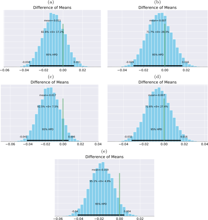

  

  Posterior distributions and 95% credible intervals of differences for log loss scores from different methods. (a) Time Series Method Alone vs NLP NSC Method Alone. (b) NLP MNB Method Alone vs Time Series Method Alone. (c) NLP MNB Method Alone vs NLP NSC Method Alone. (d) NLP MNB Combined with Time Series Features vs NLP MNB Method Alone. (e) NLP NSC Combined with Time Series Features vs NLP NSC Method Alone

• NLP MNB Method Alone vs Time Series Method Alone (Fig. 23(b)),

• NLP MNB Method Alone vs NLP NSC Method Alone (Fig. 23(c)),

• NLP MNB Combined with Time Series Features vs NLP MNB Method Alone (Fig. 23(d)),

• and NLP NSC Combined with Time Series Features vs NLP NSC Method Alone (Fig. 23(e)).

Although the p-values for the Wilcoxon Signed Rank Tests on the above pairs were all significantly smaller than 0.05, it is shown on the posterior distributions of the differences of means that zeros were all within the 95% credible intervals (Fig. 23). However, there is a 95.1% chance that the combination of language time series features with the NSC method improved the mean log loss (Fig. 23(e)).

The scores are also summarized in a critical difference diagram created using the scmamp R library [76], with a significance level of 0.05, as shown in Fig. 24. Die diagram shows that the differences between NLP MNB, NLP MNB combined with time series features, and NLP NSC combined with time series features are not statistically significant, while the NLP NSC method clearly improved from being combined with time series features.

Figure 24

Critical Difference Diagram for negative test log loss scores obtained from Time Series Method (TS NSC light preprocessing) and NLP Methods alone, and from the combined methods

7.4 Stylometric features of Hamilton’s and Madison’s papers

From the time series features selected in the Federalist Papers case study, we found that at the sentence level, token length features dominated the most statistically significant time series features. In the top ten most relevant features selected, two were token length sequence time series features and eight were token length distribution time series features. The top ten most relevant features are summarized in Appendix B.

7.4.1 Token length sequence: mean and non-linearity

The top two most significant features are

with a p-value of $9.181\cdot10^{-27}$, and

with a p-value of $1.581\cdot10^{-24}$. In this section, we will show that both features describe the differences in the mean token length between sentences, and the TLS__c3__lag_1 feature also captures some variances in non-linearity of the token length sequence time series.

The TLS__mean feature is easy to understand. It calculates the mean token length for every token length sequence. The histograms for the distributions of the feature from both Hamilton and Madison are shown in Fig. 25. Due to the imbalance in sample sizes between the two classes, both histograms are normalized.

Figure 25

Normalized distribution plot of mean token lengths for sentences Hamilton and Madison

The mean features of samples from Madison in average exceed the ones from Hamilton, suggesting that Madison’s sample sentences tend to have longer tokens than Hamilton’s sample sentences on average. The posterior distribution of the differences of means between the two distributions is well separated from zero (Fig. 26(a)), while the posterior distribution of the differences of standard deviations indicates a 94% chance that the standard deviation of Madison’s mean token lengths is larger than Hamilton’s mean token lengths (Fig. 26(b)).

Figure 26

Posterior distributions and 95% credible intervals of differences for the “mean” feature. Left is the difference of group means, and right is the difference of group standard deviations

The feature TLS__c3__lag_1 deploys a non-linearity measurement proposed in [77]:

$$ \frac{1}{n_{i}-2l} \sum_{j=1}^{n_{i}-2l}z_{i,j+2l} \cdot z_{i,j+l} \cdot z_{i,j}, $$

(22)

where $n_{i}$ is the number of tokens of the ith token length sequence, l is the lag parameter, which is 1 for the TLS__c3__lag_1 feature, and $z_{i,j}$ is the jth token length of sample i. With $l = 1$, the c3 measurement is effectively calculating the expected value of the product of three consecutive points in the token length sequence. The distributions of the feature extracted from samples from both classes show that the Madison class tends to have higher c3 measurements, as shown in Fig. 27. The distributions are both normalized to compensate for the imbalance of sample sizes between the two classes and are log-transformed.

Figure 27

Distribution plot of feature “c3__lag_1” of token length sequence time series from classes Hamilton and Madison (normalized by sample sizes and log-transformed)

Although the c3 function was proposed to measure the non-linearity of the time series, from the equation we can easily find that the measurement could be affected by the mean value of the time series. A higher mean would result in a higher c3 measurement. Therefore, to remove the effect of the differences in the mean token lengths between sentences, we normalized each token length sequence by its mean and extracted the c3 feature again. The resulting distributions are plotted in Fig. 28, where the differences between the two distributions are barely visible, suggesting that the majority of the variances in the c3 feature can be explained by the differences in the mean feature of both classes. However, analyzing the posterior distributions of the differences of means for the normalized c3 values, we found that the differences of means are still significant, where only 0.9% of the posterior distribution landed beyond zero, as shown in Fig. 29.

Figure 28

Distribution plot of the normalized-by-mean feature “c3__lag_1” of token length sequence time series from classes Hamilton and Madison (normalized by sample sizes and log-transformed)

Figure 29

Posterior distributions and 95% credible intervals of differences for the normalized-by-mean “c3__lag_1” feature. Left is the difference of group means, and right is the difference of group standard deviations

7.4.2 Token length distribution: intercept and slope of linear trend

In the top ten most statistically significant time series features, there are

at the 3rd position, with a p-value of $3.591\cdot10^{-24}$, and

at the 6th position, with a p-value of $6.720\cdot10^{-24}$. Both of these measure a specific attribution of a linear least-squares regression fitted on the values of the given token length distribution, versus the sequence from zero to the length of the sequence minus one.

A linear least-squares regression fitted on a token length distribution not only captures the differences of the mean token lengths of the sentences, but it is also dependent on the distribution as a whole and can describe how steep the distribution is. Because the token length distribution calculates frequencies of token lengths that are normalized to the number of tokens in the sentences, steepness can be described by both the intercept and the slope of the linear model, which are the TLD__linear_trend__attr_"intercept" and TLD__linear_trend__attr_"slope" features, respectively. From the plots in Fig. 30 and Fig. 31, it is clear that the intercepts calculated from length distributions of class Madison tend to be lower and the slopes tend to have higher values (less negative) than the corresponding values calculated from time series of class Hamilton. The differences in the average intercept and slope values of the fitted linear least-squares regression suggests that the token length distribution from the Madison class tend to be less “steep”, which further suggests that the lengths of the tokens in the sentences written by Madison tend to be less concentrated in lower values but more in higher values, compared to the ones from Hamilton’s writings. This finding is also supported by the fact that Madison’s writings tend to have a higher mean token length than Hamilton’s writings.

Figure 30

Distribution plot of the feature “linear_trend__attr_‘intercept’” of token length sequence time series from classes Hamilton and Madison (normalized by sample sizes)

Figure 31

Distribution plot of the feature “linear_trend__attr_‘slope’” of token length sequence time series from classes Hamilton and Madison (normalized by sample sizes)

8 Discussion

In this section, we first answer our research question by considering the results from our two case studies. We then discuss the limitations of our study and describe our repository which makes the implementation of our approach openly available.

8.1 Answer to our research question

RQ: Can time series analysis be combined with existing natural language processing methods to improve accuracy of text analysis for the authorship attribution problem?

In the Spooky Books Case Study, the results show that the systematic extraction of time series features from functional language sequences improves the predictions of a baseline NLP method for an exemplary authorship attribution problem (Fig. 8). The baseline NLP method was chosen to be a Multinomial-Naive-Bayes model, which outperformed three other established NLP models (Fig. 7). The presented feature engineering methodology generates novel types of stylometric features (Sect. 6.4), which show characteristic differences between authors (Figs. 13, 16, 19). These extracted stylometric features can be used to visualize the resemblance of writing styles between different authors for individual sentences (Fig. 4).

On the other hand, in the Federalist Papers case study, the combination of the time series features extracted from the functional language sequences showed only minor improvements of the overall performance when combined with a strong benchmark NLP method. These performance improvements were not statistically significant. However, when combined with an established NLP method, which is known for its excellent performance on the paper-wise authorship attribution problem, we observed a 95.1% chance that the suggested feature engineering approach improved the overall performance (Fig. 23), such that it become comparable to the group of best performing algorithms (Fig. 24).

Overall, on the case studies performed on two data sets presented in this work, the time series features extracted from the functional language sequences either provided extra information to effectively improve the baseline NLP methods, or achieved the same level of performance as the competing NLP methods.

8.2 Limitations

There exist a few limitations in our evaluation, to be specific, there are limitations on the data sets, and also limitations on the baseline NLP methods.

Firstly, our case studies focused specifically on authorship attribution problems with very short text samples and relatively large numbers of samples. In the Spooky Books data set, the text samples are individual sentences split from books of the same genre—spooky novels - written by three authors. In the Federalist Papers data set, the text samples are sentences from the famous Federalist Papers written by Hamilton and Madison—who were the potential writers of the twelve disputed Federalist Papers and share many similarities in their writings. To the best of our knowledge, authorship attribution tasks on sentence level text samples have not been discussed in the literature. The two case studies have shown the strength of the proposed language time series enhanced authorship attribution method on two data sets with very short text samples and share the same genre or topic. However, there remains further studies on how the proposed method will perform on other authorship attribution problems with longer texts, more candidate authors, cross-genre texts, other forms of documents such as messages or tweets, or even on other authorship analysis problems including authorship verification and authorship profiling.

Secondly, due to the lack of literature on authorship attribution methods working with very short text samples, there is no guarantee that the selected baseline NLP methods in the two case studies were the most suitable and state-of-art methods for the selected data sets. Instead, the selected NLP methods were the best or the most widely used ones we could find for the case studies. In the Spooky Books case study, we selected and experimented with five advanced NLP methods as baselines, from which one was rejected due to requirements on computational performance. In the Federalist Papers case study, we directly compared the proposed method with the NSC method (Sect. 7.2), which successfully classified the known authors for the Federalist Papers with zero classification error for the paper-wise authorship attribution problem. However, these results were obtained at an article level, which contains much more tokens per text sample than that at a sentence level. The best NLP method observed in the Spooky Books case study was also added to the comparison in the Federalist Papers case study, and the method outperformed the NSC method (Fig. 23). It is possible that there are more suitable or advanced methods that could have been used as baselines in this study that we have missed. However, we have shown that our proposed method is able to improve the predictions over these selected baselines.

The presented feature engineering approach has a large space to be further explored and improved. E.g., our results are not as competitive as the results, which were achieved by the winning teams of Kaggle’s Spooky Author Identification competition. However, as the information about the methods used by the winning teams are not publicly accessible; we are not able to systematically compare our approach with theirs. Another possible improvement could be achieved by combining our feature selection approach with other established feature selection approaches, which basically would form a second tier of feature selection.

Due to limited time, we have only studied five basic mapping methods for generating functional language sequence, which mainly extended the existing literature on language time series analysis. There also exists a wide range of other methods we have not implemented. As an example, part-of-speech (POS) tagging is a common transformation method used in text analysis and contains stylometric features of the texts. A text can be transformed into a continuous sequence of POS tags, which gives a wide berth for functional language sequences to be constructed using different mapping methods. Similarly, there are also existing text preprocessing and transformation methods that can be used in developing functional language sequence mapping methods.

Given these limitations, there remain many aspects of our approach to be further explored but due to limited time and scope for this study, we were not able to include these aspects into this single work. This opens up many avenues for future work including applying our methods to additional data sets, comparing our methods to other baselines, expanding our feature selection approach, and developing additional mapping methods.

8.3 Open implementation of our methods

To enable other researchers to use and experiment with different methods on different data sets and to explore more properties of this approach, we published our implementation of our approach in a GitHub repository⁵ under the MIT license. This will enable other researchers to replicate our results and potentially apply our approach to other authorship attribution problems.

9 Conclusion

We have introduced a consistent mathematical framework, which combines established methods for the generation of language time series with methods for the generation of functional language sequences. The framework also models the systematic feature engineering based on approaches from time series classification, which includes a statistical testing methodology for multi-classification problems. In total, 3970 novel stylometric features have been evaluated with respect to their ability to improve the authorship attribution problem of our case studies.

The main contribution of this paper is a novel feature extraction approach for natural language text that combines methods from Times Series Classification, Functional Data Analysis, and automated Time Series feature extraction with existing Natural Language Processing techniques. We call this approach Functional Language Analysis. This approach enables complete sentences to be considered when extracting features from natural text.

Applying our Functional Language Analysis approach to the sentence-wise authorship attribution problem has demonstrated that it is able to extract statistically significant features, which can improve existing techniques for analyzing natural text. Further, for authorship attribution, a novel visualization technique is introduced which allows differences and commonalities of stylometric features in natural text to be easily viewed. In summary, this research opens the door to an exciting new line of research which merges two distinct fields of machine learning.

Appendices

Appendix A: Most relevant features extracted from each mapping method for the Spooky Books Data Set

The following section summarizes ten of the most relevant time series features, which have been extracted from the functional language sequences discussed in Sect. 3.3. The reported p-value is the maximum of the three hypothesis tests (Algorithm 1) conducted for every feature in the course of the feature selection (Eq. (15)). Due to the univariate hypothesis testing and the similarities in generating the sequences, many of the reported features are colinear.

1.1 A.1 Exemplary features from token length sequences (TLS)

1.1.1 A.1.1 Aggregated linear trend

Maximal p -value :

$6.524\cdot10^{-21}$

Feature name :

Description :

The minimal intercept of linear regression models, which were fitted to chunks of 10 time series values.

1.1.2 A.1.2 Quantile

Maximal p -value :

$6.650\cdot10^{-21}$

Feature name :

Description :

The value at the 10th percentile.

1.1.3 A.1.3 Nonlinearity

Maximal p -value :

$3.340\cdot10^{-20}$

Feature name :

Description :

A measurement of nonlinearity [77] with a lag value of 1.

1.1.4 A.1.4 Aggregated linear trend

Maximal p -value :

$2.255\cdot10^{-19}$

Feature name :

Description :

The minimal standard error of linear regression models, which were fitted to chunks of 10 time series values.

1.1.5 A.1.5 Aggregated linear trend

Maximal p -value :

$6.393\cdot10^{-17}$

Feature name :

Description :

The minimal intercept of linear regression models, which were fitted to chunks of 5 time series values.

1.1.6 A.1.6 Median

Maximal p -value :

$3.447\cdot10^{-11}$

Feature name :

Description :

The median of the time series values.

1.1.7 A.1.7 Mean

Maximal p -value :

$1.369\cdot10^{-09}$

Feature name :

Description :

The mean of the time series values.

1.1.8 A.1.8 Change quantiles

Maximal p -value :

$1.548\cdot10^{-09}$

Feature name :

Description :

The variance of absolute differences between consecutive time series values, which are larger than the 80th percentile.

1.1.9 A.1.9 Change quantiles

Maximal p -value :

$1.570\cdot10^{-09}$

Feature name :

Description :

The variance of differences between consecutive time series values, which are larger than the 80th percentile.

1.1.10 A.1.10 Change quantiles

Maximal p -value :

$4.119\cdot10^{-09}$

Feature name :

Description :

The mean differences between consecutive time series values, which are smaller than the 60th percentile.

1.2 A.2 Exemplary features from token frequency sequences (TFS)

1.2.1 A.2.1 Change quantiles

Maximal p -value :

$2.502\cdot10^{-36}$

Feature name :

Description :

The mean absolute differences between consecutive time series values, which are smaller than the 60th percentile.

1.2.2 A.2.2 Quantile

Maximal p -value :

$1.734\cdot10^{-34}$

Feature name :

Description :

The value at the 30th percentile.

1.2.3 A.2.3 Median

Maximal p -value :

$3.440\cdot10^{-34}$

Feature name :

Description :

The median of all values in the time series.

1.2.4 A.2.4 Quantile

Maximal p -value :

$5.097\cdot10^{-31}$

Feature name :

Description :

The value at the 40th percentile.

1.2.5 A.2.5 Last maximum

Maximal p -value :

$2.519\cdot10^{-23}$

Feature name :

Description :

The relative last location of the maximum value of the time series.

1.2.6 A.2.6 Variance

Maximal p -value :

$1.066\cdot10^{-19}$

Feature name :

Description :

The variane of all values in the time series.

1.2.7 A.2.7 Standard deviation

Maximal p -value :

$1.066\cdot10^{-19}$

Feature name :

Description :

The standard deviation of all values in the time series.

1.2.8 A.2.8 Aggregated linear trend

Maximal p -value :

$1.706\cdot10^{-19}$

Feature name :

Description :

The variance of intercepts, which were obtained from linear regression models being fitted to chunks of 10 time series values.

1.2.9 A.2.9 Ratio beyond r sigma

Maximal p -value :

$6.935\cdot10^{-19}$

Feature name :

Description :

The ratio of values that are more than $1.5 \cdot \operatorname{std}(x)$ away from the mean of x where x is the target time series.

1.2.10 A.2.10 Quantile

Maximal p -value :

$1.010\cdot10^{-18}$

Feature name :

Description :

The value at the 20th percentile.

1.3 A.3 Exemplary features from token rank sequences (TRS)

1.3.1 A.3.1 Median

Maximal p -value :

$1.463\cdot10^{-34}$

Feature name :

Description :

The median of all values in the time series.

1.3.2 A.3.2 Quantile

Maximal p -value :

$2.376\cdot10^{-34}$

Feature name :

Description :

The value at the 60th percentile.

1.3.3 A.3.3 Wavelet coefficient

Maximal p -value :

$5.044\cdot10^{-33}$

Feature name :

Description :

The 0 coefficient for the Continuous wavelet transform for the Ricker wavelet with a width parameter of 20.

1.3.4 A.3.4 Wavelet coefficient

Maximal p -value :

$5.319\cdot10^{-29}$

Feature name :

Description :

The 1 coefficient for the Continuous wavelet transform for the Ricker wavelet with a width parameter of 20.

1.3.5 A.3.5 Change quantiles

Maximal p -value :

$2.878\cdot10^{-27}$

Feature name :

Description :

The variance of differences between consecutive TRS values, if the respective TRS values were larger than the 20th percentile and smaller than the 80th percentile.

1.3.6 A.3.6 Change quantiles

Maximal p -value :

$3.540\cdot10^{-27}$

Feature name :

Description :

The variance of absolute differences between consecutive TRS values, if the respective TRS values were larger than the 40th percentile and smaller than the 80th percentile.

1.3.7 A.3.7 Change quantiles

Maximal p -value :

$2.062\cdot10^{-26}$

Feature name :

Description :

The variance of the absolute consecutive changes inside a corridor between 0th and 60th percentile.

1.3.8 A.3.8 Change quantiles

Maximal p -value :

$2.709\cdot10^{-25}$

Feature name :

Description :

The variance of the absolute consecutive changes inside a corridor between 20th and 80th percentile.

1.3.9 A.3.9 Change quantiles

Maximal p -value :

$1.812\cdot10^{-24}$

Feature name :

Description :

The variance of the consecutive changes inside a corridor between 60th and 100th percentile.

1.3.10 A.3.10 Change quantiles

Maximal p -value :

$2.009\cdot10^{-24}$

Feature name :

Description :

The average of the absolute consecutive changes inside a corridor between 0th and 60th percentile.

1.4 A.4 Exemplary features from token length distributions (TLD)

1.4.1 A.4.1 Index of mass quantile

Maximal p -value :

$1.311\cdot10^{-19}$

Feature name :

Description :

The relative index where 10% of the mass of the time series lie behind.

1.4.2 A.4.2 Change quantiles

Maximal p -value :

$5.621\cdot10^{-15}$

Feature name :

Description :

The average of the consecutive changes inside a corridor between 40th and 100th percentile.

1.4.3 A.4.3 Change quantiles

Maximal p -value :

$5.020\cdot10^{-14}$

Feature name :

Description :

The average of the consecutive changes inside a corridor between 20th and 100th percentile.

1.4.4 A.4.4 Energy ratio by chunks

Maximal p -value :

$1.678\cdot10^{-13}$

Feature name :

Description :

The sum of squares of values in the first chunk out of 10, as a ratio with the value over the whole time series.

1.4.5 A.4.5 Change quantiles

Maximal p -value :

$2.644\cdot10^{-13}$

Feature name :

Description :

The average of the consecutive changes inside a corridor between 0th and 100th percentile.

1.4.6 A.4.6 Mean change

Maximal p -value :

$2.644\cdot10^{-13}$

Feature name :

Description :

The mean over the differences between subsequent time series values.

1.4.7 A.4.7 Wavelet coefficient

Maximal p -value :

$5.597\cdot10^{-12}$

Feature name :

Description :

The 8 coefficient for the Continuous wavelet transform for the Ricker wavelet with a width parameter of 20.

1.4.8 A.4.8 FFT coefficient

Maximal p -value :

$1.649\cdot10^{-11}$

Feature name :

Description :

The angle of the 2nd Fourier coefficient of the one-dimensional discrete Fourier Transform.

1.4.9 A.4.9 FFT coefficient

Maximal p -value :

$2.197\cdot10^{-11}$

Feature name :

Description :

The real part of the 2nd Fourier coefficient of the one-dimensional discrete Fourier Transform.

1.4.10 A.4.10 Wavelet coefficient

Maximal p -value :

$4.276\cdot10^{-10}$

Feature name :

Description :

The 10 coefficient for the Continuous wavelet transform for the Ricker wavelet with a width parameter of 20.

1.5 A.5 Exemplary features from token range distributions (TRD)

1.5.1 A.5.1 FFT coefficient

Maximal p -value :

$2.756\cdot10^{-25}$

Feature name :

Description :

The imaginary part of the 84th Fourier coefficient of the one-dimensional discrete Fourier Transform.

1.5.2 A.5.2 FFT coefficient

Maximal p -value :

$1.895\cdot10^{-24}$

Feature name :

Description :

The imaginary part of the 21st Fourier coefficient of the one-dimensional discrete Fourier Transform.

1.5.3 A.5.3 FFT coefficient

Maximal p -value :

$4.802\cdot10^{-22}$

Feature name :

Description :

The imaginary part of the 14th Fourier coefficient of the one-dimensional discrete Fourier Transform.

1.5.4 A.5.4 FFT coefficient

Maximal p -value :

$1.064\cdot10^{-18}$

Feature name :

Description :

The imaginary part of the 92nd Fourier coefficient of the one-dimensional discrete Fourier Transform.

1.5.5 A.5.5 Aggregated linear trend

Maximal p -value :

$5.872\cdot10^{-16}$

Feature name :

Description :

The maximal intercept of linear regression models, which were fitted to chunks of 10 time series values.

1.5.6 A.5.6 FFT coefficient

Maximal p -value :

$6.450\cdot10^{-16}$

Feature name :

Description :

The imaginary part of the 8th Fourier coefficient of the one-dimensional discrete Fourier Transform.

1.5.7 A.5.7 Number of peaks

Maximal p -value :

$1.638\cdot10^{-15}$

Feature name :

Description :

The number of peaks of at least support 3 in the time series.

1.5.8 A.5.8 FFT coefficient

Maximal p -value :

$2.277\cdot10^{-15}$

Feature name :

Description :

The real part of the 65th Fourier coefficient of the one-dimensional discrete Fourier Transform.

1.5.9 A.5.9 Ratio beyond r sigma

Maximal p -value :

$4.396\cdot10^{-15}$

Feature name :

Description :

The ratio of values that are more than $2.5 \cdot\operatorname{std}(x)$ away from the mean of the individual sequence.

1.5.10 A.5.10 Approximate entropy

Maximal p -value :

$4.775\cdot10^{-15}$

Feature name :

Description :

The approximate entropy calculated with a length 2 of compared run of data and a 0.9 filtering level.

Appendix B: Most relevant features extracted from the Federalist Papers Data Set

The following section summarizes the top ten most relevant time series features extracted from the Federalist Papers Data Set, using four functional language sequences mapping methods discussed in Sect. 3.3, including token length sequence, token frequency sequence, token rank sequence and token length distribution. The classification task was binary, hence the p-values of the hypothesis tests are equal for both classes and are reported in this section.

2.1 B.1 C3

Method :

Token length sequence

p -value :

$9.181\cdot10^{-27}$

Feature name :

Description :

A measurement of nonlinearity [77] with a lag value of 1.

2.2 B.2 Mean

Method :

Token length sequence

p -value :

$1.581\cdot10^{-24}$

Feature name :

Description :

The mean of all values in the time series.

2.3 B.3 Linear trend

Method :

Token length distribution

p -value :

$3.591\cdot10^{-24}$

Feature name :

Description :

The intercept of a linear least-squares regression fit on values of the time series versus the sequence from 0 to length of the time series minus one.

2.4 B.4 Wavelet coefficient

Method :

Token length distribution

p -value :

$5.211\cdot10^{-24}$

Feature name :

Description :

The 12 coefficient for the Continuous wavelet transform for the Ricker wavelet with a width parameter of 20.

2.5 B.5 Wavelet coefficient

Method :

Token length distribution

p -value :

$6.689\cdot10^{-24}$

Feature name :

Description :

The 0 coefficient for the Continuous wavelet transform for the Ricker wavelet with a width parameter of 10.

2.6 B.6 Linear trend

Method :

Token length distribution

p -value :

$6.720\cdot10^{-24}$

Feature name :

Description :

The slope of a linear least-squares regression fit on values of the time series versus the sequence from 0 to length of the time series minus one.

2.7 B.7 Wavelet coefficient

Method :

Token length distribution

p -value :

$2.196\cdot10^{-23}$

Feature name :

Description :

The 12 coefficient for the Continuous wavelet transform for the Ricker wavelet with a width parameter of 10.

2.8 B.8 Wavelet coefficient

Method :

Token length distribution

p -value :

$4.470\cdot10^{-23}$

Feature name :

Description :

The 2 coefficient for the Continuous wavelet transform for the Ricker wavelet with a width parameter of 5.

2.9 B.9 Wavelet coefficient

Method :

Token length distribution

p -value :

$1.860\cdot10^{-22}$

Feature name :

Description :

The 1 coefficient for the Continuous wavelet transform for the Ricker wavelet with a width parameter of 5.

2.10 B.10 Wavelet coefficient

Method :

Token length distribution

p -value :

$1.245\cdot10^{-21}$

Feature name :

Description :

The 11 coefficient for the Continuous wavelet transform for the Ricker wavelet with a width parameter of 10.

References

Rabiner LR, Juang B-H (1993) Fundamentals of speech recognition. Prentice Hall, Englewood Cliffs
Rocha A, Scheirer WJ, Forstall CW, Cavalcante T, Theophilo A, Shen B, Carvalho ARB, Stamatatos E (2017) Authorship attribution for social media forensics. IEEE Trans Inf Forensics Secur 12(1):5–33. https://doi.org/10.1109/TIFS.2016.2603960
Fan Z-P, Che Y-J, Chen Z-Y (2017) Product sales forecasting using online reviews and historical sales data: a method combining the Bass model and sentiment analysis. J Bus Res 74:90–100. https://doi.org/10.1016/j.jbusres.2017.01.010
Skuza M, Romanowski A (2015) Sentiment analysis of Twitter data within big data distributed environment for stock prediction. In: Ganzha M, Maciaszek L, Paprzycki M (eds) Proceedings of the federated conference on computer science and information systems. Annals of computer science and information systems, vol 5. Polish Information Processing Society, Warsaw; IEEE, Los Alamitos, pp 1349–1354. https://doi.org/10.15439/2015F230
Jensen PB, Jensen LJ, Brunak S (2012) Mining electronic health records: towards better research applications and clinical care. Nat Rev Genet 13:395–405. https://doi.org/10.1038/nrg3208
Nakada T, Fujii Y, Yoneoka Y, Kwee IL (2001) Planum temporale: where spoken and written language meet. Eur Neurol 46(3):121–125. https://doi.org/10.1159/000050784
Kupiec J (1992) Robust part-of-speech tagging using a hidden Markov model. Comput Speech Lang 6(3):225–242. https://doi.org/10.1016/0885-2308(92)90019-Z
Stamatatos E (2016) Universality of stylistic traits in texts. In: Esposti MD, Altmann EG, Pachet F (eds) Creativity and universality in language. Lecture notes in morphogenesis. Springer, Cham, pp 143–155. https://doi.org/10.1007/978-3-319-24403-7_9
Stamatatos E (2009) A survey of modern authorship attribution methods. J Am Soc Inf Sci Technol 60(3):538–556
Fulcher BD (2018) Feature-based time-series analysis. In: Dong G, Liu H (eds) Feature engineering for machine learning and data analytics. Taylor & Francis, Boca Raton, pp 87–116
Christ M, Kempa-Liehr AW, Feindt M (2016) Distributed and parallel time series feature extraction for industrial big data applications. arXiv:1610.07717v1
Christ M, Braun N, Neuffer J, Kempa-Liehr AW (2018) Time Series FeatuRe Extraction on basis of Scalable Hypothesis tests (tsfresh—a Python package). Neurocomputing 307:72–77
Kosmidis K, Kalampokis A, Argyrakis P (2006) Language time series analysis. Phys A, Stat Mech Appl 370(2):808–816. https://doi.org/10.1016/j.physa.2006.02.042
Wang J-L, Chiou J-M, Müller H-G (2016) Functional data analysis. Annu Rev Stat Appl 3:257–295. https://doi.org/10.1146/annurev-statistics-041715-033624
Tweedie FJ, Singh S, Holmes DI (1996) Neural network applications in stylometry: The Federalist Papers. Comput Humanit 30(1):1–10
Jockers ML, Witten DM (2010) A comparative study of machine learning methods for authorship attribution. Lit Linguist Comput 25(2):215–223. https://doi.org/10.1093/llc/fqq001
Kaggle (2018) Spooky author identification. https://www.kaggle.com/c/spooky-author-identification/data
Fang X, Zhan J (2015) Sentiment analysis using product review data. J Big Data 2(1):5. https://doi.org/10.1186/s40537-015-0015-2
Huang W, Nakamori Y, Wang S-Y (2005) Forecasting stock market movement direction with support vector machine. Comput Oper Res 32(10):2513–2522. https://doi.org/10.1016/j.cor.2004.03.016
Ignatov A (2018) Real-time human activity recognition from accelerometer data using convolutional neural networks. Appl Soft Comput 62:915–922. https://doi.org/10.1016/j.asoc.2017.09.027
Ramsay JO, Silverman BW (2005) Functional data analysis, 2nd edn. Springer series in statistics. Springer, Berlin. https://doi.org/10.1007/b98888
Bagnall A, Lines J, Bostrom A, Large J, Keogh E (2017) The great time series classification bake off: a review and experimental evaluation of recent algorithmic advances. Data Min Knowl Discov 31:606–660 https://doi.org/10.1007/s10618-016-0483-9
Montemurro MA, Pury PA (2002) Long-range fractal correlations in literary corpora. Fractals 10(4):451–461
Ausloos M (2012) Generalized Hurst exponent and multifractal function of original and translated texts mapped into frequency and length time series. Phys Rev E 86(3):031108
Kalimeri M, Constantoudis V, Papadimitriou C, Karamanos K, Diakonos FK, Papageorgiou H (2012) Entropy analysis of word-length series of natural language texts: effects of text language and genre. Int J Bifurc Chaos 22(9):1250223
Tanaka-Ishii K, Bunde A (2016) Long-range memory in literary texts: on the universal clustering of the rare words. PLoS ONE 11(11):e0164658
Mendenhall TC (1887) The characteristic curves of composition. Science 9(214):237–249
Chaski CE (2005) Who’s at the keyboard? Authorship attribution in digital evidence investigations. Int J Digit Evid 4(1):1–13
Stamatatos E, Fakotakis N, Kokkinakis G (2000) Automatic text categorization in terms of genre and author. Comput Linguist 26(4):471–495
Tambouratzis G, Markantonatou S, Hairetakis N, Vassiliou M, Carayannis G, Tambouratzis D (2004) Discriminating the registers and styles in the modern Greek language—part 2: extending the feature vector to optimize author discrimination. Lit Linguist Comput 19(2):221–242
Diederich J, Kindermann J, Leopold E, Paass G (2003) Authorship attribution with support vector machines. Appl Intell 19(1–2):109–123
Li J, Zheng R, Chen H (2006) From fingerprint to writeprint. Commun ACM 49(4):76–82
Sanderson C, Guenter S (2006) Short text authorship attribution via sequence kernels, Markov chains and author unmasking: an investigation. In: Proceedings of the 2006 conference on empirical methods in natural language processing. Association for Computational Linguistics, Stroudsburg, pp 482–491
Uzuner Ö, Katz B (2005) A comparative study of language models for book and author recognition. In: International conference on natural language processing. Springer, Berlin, pp 969–980
Khosmood F, Levinson R (2006) Toward unification of source attribution processes and techniques. In: 2006 international conference on machine learning and cybernetics, pp 4551–4556
Matthews RA, Merriam TV (1993) Neural computation in stylometry I: an application to the works of Shakespeare and Fletcher. Lit Linguist Comput 8(4):203–209
Luyckx K, Daelemans W (2005) Shallow text analysis and machine learning for authorship attribution. In: Computational linguistics in the Netherlands 2004: selected papers from the fifteenth CLIN meeting. LOT, Utrecht, pp 149–160
Stamatatos E (2006) Authorship attribution based on feature set subspacing ensembles. Int J Artif Intell Tools 15(5):823–838
Hirst G, Feiguina O (2007) Bigrams of syntactic labels for authorship discrimination of short texts. Lit Linguist Comput 22(4):405–417
Mosteller F, Wallace DL (1984) Applied Bayesian and classical inference. The case of The Federalist Papers, 2nd edn. Springer, New York. https://doi.org/10.1007/978-1-4612-5256-6
Ding SH, Fung BC, Iqbal F, Cheung WK (2017) Learning stylometric representations for authorship analysis. IEEE Trans Cybern 49:107–121
Kernot D, Bossomaier T, Bradbury R (2018) Using Shakespeare’s sotto voce to determine true identity from text. Front Psychol 9:289
Mehri A, Darooneh AH, Shariati A (2012) The complex networks approach for authorship attribution of books. Phys A, Stat Mech Appl 391(7):2429–2437
Akimushkin C, Amancio DR, Oliveira ON Jr (2018) On the role of words in the network structure of texts: application to authorship attribution. Phys A, Stat Mech Appl 495:49–58
Machicao J, Corrêa EA Jr, Miranda GH, Amancio DR, Bruno OM (2018) Authorship attribution based on life-like network automata. PLoS ONE 13(3):e0193703
Al Rozz Y, Menezes R (2018) Author attribution using network motifs. In: Cornelius S, Coronges K, Goncalves B, Sinatra R, Vespignani A (eds) Complex networks IX. Springer proceedings in complexity, pp 199–207
Kestemont M, Tschuggnall M, Stamatatos E, Daelemans W, Specht G, Stein B, Potthast M (2018) Overview of the author identification task at PAN-2018: cross-domain authorship attribution and style change detection. In: Working notes of CLEF 2018—conference and labs of the evaluation forum
Martinčić-Ipšić S, Margan D, Meštrović A (2016) Multilayer network of language: a unified framework for structural analysis of linguistic subsystems. Phys A, Stat Mech Appl 457:117–128
Amancio DR, Aluisio SM, Oliveira ON Jr, Costa LdF (2012) Complex networks analysis of language complexity. Europhys Lett 100(5):58002
Riedl M, Biemann C (2018) Using semantics for granularities of tokenization. Comput Linguist 44(3):483–524. https://doi.org/10.1162/coli_a_00325
Dhar V (2013) Data science and prediction. Commun ACM 56(12):64–73. https://doi.org/10.1145/2500499
Mann HB, Whitney DR (1947) On a test of whether one of two random variables is stochastically larger than the other. Ann Math Stat 18(1):50–60
Lehmann EL (1951) Consistency and unbiasedness of certain nonparametric tests. Ann Math Stat 22(2):165–179
Fay MP, Proschan MA (2010) Wilcoxon–Mann–Whitney or t-test? On assumptions for hypothesis tests and multiple interpretations of decision rules. Stat Surv 4:1–39. https://doi.org/10.1214/09-SS051
Benjamini Y, Hochberg Y (1995) Controlling the false discovery rate: a practical and powerful approach to multiple testing. J R Stat Soc, Ser B, Methodol 57:289–300
Rodriguez E, Aguilar-Cornejo M, Femat R, Alvarez-Ramirez J (2014) Scale and time dependence of serial correlations in word-length time series of written texts. Phys A, Stat Mech Appl 414:378–386
Guzmán-Vargas L, Obregón-Quintana B, Aguilar-Velázquez D, Hernández-Pérez R, Liebovitch LS (2015) Word-length correlations and memory in large texts: a visibility network analysis. Entropy 17(11):7798–7810
Constantoudis V, Kalimeri M, Diakonos F, Karamanos K, Papadimitriou C, Chatzigeorgiou M, Papageorgiou H (2016) Long-range correlations and burstiness in written texts: universal and language-specific aspects. Int J Mod Phys B 30(15):1541005
Pietraszewska N (2015) On the complexity of creole languages: the fractal approach. Acad J Mod Philol 4:73–80
Deng W, Wang D, Li W, Wang QA (2011) English and Chinese language frequency time series analysis. Chin Sci Bull 56(34):3717–3722
Hamilton A, Jay J, Madison J (1998) The Project Gutenberg EBook of The Federalist Papers. EBook, vol 1404. Project Gutenberg Literary Archive Foundation, Salt Lake City. http://www.gutenberg.org/ebooks/1404
Shelley MWG (2018) Frankenstein; or, the modern Prometheus. EBook, vol 84. Project Gutenberg Literary Archive Foundation, Salt Lake City. http://www.gutenberg.org/files/84/84-h/84-h.htm
Loper E, Klein E, Bird S (2015) Natural language processing with Python. University of Melbourne, Melbourne. http://www.nltk.org/book
Pedregosa F, Varoquaux G, Gramfort A, Michel V, Thirion B, Grisel O, Blondel M, Prettenhofer P, Weiss R, Dubourg V, Vanderplas J, Passos A, Cournapeau D, Brucher M, Perrot M, Duchesnay E (2011) Scikit-learn: machine learning in Python. J Mach Learn Res 12:2825–2830
Kumar P (2019) Copula functions and applications in engineering. In: Deep K, Jain M, Salhi S (eds) Logistics, supply chain and financial predictive analytics Springer, Singapore, pp 195–209. https://doi.org/10.1007/978-981-13-0872-7_15
McKinney W (2010) Data structures for statistical computing in Python. In: Proceedings of the 9th Python in science conference, pp 56–61.
Chen T, Guestrin C (2016) XGBoost: a scalable tree boosting system. In: Proceedings of the 22nd ACM SIGKDD international conference on knowledge discovery and data mining. ACM, New York, pp 785–794
Custódio JE, Paraboni I (2018) EACH-USP ensemble cross-domain authorship attribution. In: Working notes of CLEF 2018—conference and labs of the evaluation forum
Kruschke JK (2013) Bayesian estimation supersedes the t test. J Exp Psychol Gen 142(2):573–603
Wilcoxon F (1945) Individual comparisons by ranking methods. Biom Bull 1(6):80–83
Salvatier J, Wiecki TV, Fonnesbeck C (2016) Probabilistic programming in Python using PyMC3. PeerJ Comput Sci 2:e55
Wiecki T, Fonnesbeck C (2015) Bayesian estimation supersedes the t-test. https://docs.pymc.io/notebooks/BEST.html
Virtanen P, Gommers R, Oliphant TE, Haberland M, Reddy T, Cournapeau D, Burovski E, Peterson P, Weckesser W, Bright J, van der Walt SJ, Brett M, Wilson J, Millman KJ, Mayorov N, Nelson ARJ, Jones E, Kern R, Larson E, Carey CJ, Polat İ, Feng Y, Moore EW, VanderPlas J, Laxalde D, Perktold J, Cimrman R, Henriksen I, Quintero EA, Harris CR, Archibald AM, Ribeiro AH, Pedregosa F, van Mulbregt P, Contributors (2020) SciPy 1.0: Fundamental algorithms for scientific computing in Python. Nat Methods 17:261–272. https://doi.org/10.1038/s41592-019-0686-2
Tibshirani R, Hastie T, Narasimhan B, Chu G (2002) Diagnosis of multiple cancer types by shrunken centroids of gene expression. Proc Natl Acad Sci USA 99(10):6567–6572.
Tibshirani R, Hastie T, Narasimhan B, Chu G (2003) Class prediction by nearest shrunken centroids, with applications to DNA microarrays. Stat Sci 18(1):104–117
Calvo B, Santafe G (2015) scmamp: statistical comparison of multiple algorithms in multiple problems. R J (accepted for publication)
Schreiber T, Schmitz A (1997) Discrimination power of measures for nonlinearity in a time series. Phys Rev E 55(5):5443–5447
Acknowledgements
The authors wish to acknowledge the use of New Zealand eScience Infrastructure (NeSI) high performance computing facilities as part of this research. New Zealand’s national facilities are provided by NeSI and funded jointly by NeSI’s collaborator institutions and through the Ministry of Business, Innovation & Employment’s Research Infrastructure programme. https://www.nesi.org.nz. This research was also supported by use of the Nectar Research Cloud and by The University of Auckland. The Nectar Research Cloud is a Collaborative Australian research platform supported by the National Collaborative Research Infrastructure Strategy.
Availability of data and materials
Data are available from [17] and [61]. The source code is available at https://github.com/YichenTang97/LanTiSEAA/tree/paper_reference.
Funding
This research was supported by the Faculty of Engineering of the University of Auckland.
Author information
Authors and Affiliations
Contributions
All authors conceived the framework and the analysis and the presented case study. KB and AKL elaborated the theoretical models. YT and AKL implemented the framework and performed the analysis of the case studies. All authors analyzed and discussed the results and contributed to the manuscript. All authors read and approved the final manuscript.
Corresponding author
Ethics declarations
Competing interests
The authors declare that they have no competing interests.