The typical complexities of time-varying exposures, and by extension doses, generally require the creation of summary exposure measures. When addressing the question of the appropriate form of the summary measure of exposure, one is made aware of the strengths and limitations of whichever exposure classifications are available. An essential consideration in the choice of a summary measure of exposure is the time pattern of the effects of exposure. For some exposures and outcomes the effects may be almost instantaneous (for example, acute toxicity), whereas in other instances (for example, occupational cancer) it may take many years for the clinical effects of exposure to occur and be observed. These temporal dynamics can lead to serious exposure misclassification if ignored or misunderstood.

Taking account of biological variability when studying the effects of a chemical exposure is not a new idea. Important contributions to this field were made by Roach in the 1960s and 1970s.^1,2 Roach showed how the rate of clearance of a chemical from the body could interact with the environmental variability of the exposure to determine the toxic effects.^2,3 These ideas were further developed into a comprehensive biologically-based perspective on exposure sampling by Rappaport and colleagues.^4–6 Smith and colleagues also raised these issues in the 1980s, particularly focusing on the limitations of standard but overly simplified metrics like cumulative exposure.^7,8

In this article we present concepts and methods that may be useful in the modelling of exposure–risk relations in occupational epidemiology, and especially in the formulation and application of quantitative summary measures of exposure or dose.⁹ We also present several examples from the recent literature which illustrate these points.

FROM EXPOSURE TO DOSE: DEFINITIONS

In almost every epidemiological study, exposure is a complex, time-varying quantity that must be summarised before it can be used for exposure–response modelling. Thus, for worker i in a cohort exposed for a fixed time interval to a potentially hazardous agent, the exposure history of that worker from the beginning of exposure until the event of interest—the onset of some physiological dysfunction, disease diagnosis or death—at time T can be summarised in a vector as follows:

where x_it is the exposure level for worker i in time periods t = 1,2,3...n_i, and n_i is the number of time periods of exposure of the worker i prior to T. Most summary measures of exposure used in epidemiology are summarised from the vector

For example, cumulative exposure (CE) can be derived from the exposure vector:

Exposures must enter a target organ and reach critical concentrations before injury can occur. For a subject with an ongoing exposure, there is a profile of tissue concentrations (burdens) varying over time in a way that is analogous to an exposure profile:

where b_it is the tissue burden for worker i in time periods t = 1,2,3...n_i, and n_i is the number of time periods of exposure of the subject i prior to T. The dose (D), analogous to cumulative exposure, is therefore the time integral of the burden vector:

Burden and dose are sometimes directly measurable using biomarkers (for example, in vivo x ray fluorescence measurement of cadmium in the kidney cortex), but in most studies this is not feasible or economical.

SUMMARY MEASURES OF EXPOSURE

Cumulative exposure, the time integral of exposure intensity (equation 2), is a commonly used summary measure in occupational epidemiology. There are good reasons for this. First, taking the example of an inhaled dust with the lung as the target organ, cumulative exposure will be proportional to dose in the target organ if one assumes that ventilation rates are constant over time and similar among members of the cohort, and that the fraction of the inhaled particles deposited is also roughly constant over time and among subjects.⁷ Second, target organ dose is often assumed to be directly proportional to biological damage and disease risk. This appears to be a valid assumption for a wide variety of disease mechanisms, although we will discuss some exceptions later. Third, cumulative exposure has been shown to correlate strongly with disease risk in a wide variety of exposure–response associations.¹⁰

Other common summary measures of exposure include the average, duration of exposure, and “peak” exposure (table 1). Each of these will be appropriate for certain exposure–disease processes, but not for others. To understand this fit of exposure metric to disease process, it may be helpful to consider that the “black box” between exposure and disease involves two linked dynamic processes: the exposure–dose relation, and the dose–response relation, and that what is typically measured epidemiologically is the exposure–disease relation. Before selecting a summary measure of exposure for an epidemiological study, it is important to consider these two steps, and if possible, to have explicit hypotheses about the nature of these two relations as a means of minimising exposure misclassification.

To illustrate, consider a study of occupational exposure to power frequency electromagnetic fields and risk of brain cancer. Because of low cost microelectronics, it is relatively inexpensive to conduct a fairly extensive exposure assessment for such a study. A number of large scale studies have been conducted in which personal measurements were obtained for cases and controls, or on representative samples of workers in various jobs.^11,12 The ability to collect large numbers of measurements, including continuous profiles of intensity over periods of time, is not a common situation in occupational epidemiology, in which it is often the case that relatively few measurements are available, and each one entails substantial time and economic costs for collection and analysis. Availability of large quantities of exposure data highlights the challenge of selecting among the most appropriate exposure metric from options that might include cumulative exposure, duration, average intensity, peak and various time-specific measures of each of these. Choosing the most suitable metric is easiest when there is a strong hypothesis about the biological mechanism by which the agent (in this case electromagnetic fields) may act, although exploratory exposure/response analyses involving alternative metrics may be necessary in the absence of mechanistic knowledge.¹³

If cumulative exposure is assumed to be proportional to risk, then it follows that subjects with very different patterns of exposure over time may have the same risk, as long as the products of each subject’s average intensity and total duration of exposure are the same. This assumption holds well for cumulative damage processes—those in which each unit of dose induces tissue or cell injury, and hence increases risk, by a constant amount. For example, it is approximately true that each “pack-year” of smoking (a cumulative exposure measure: the number of packs of cigarettes smoked per day multiplied by the number of years of smoking) causes a fixed amount of loss in pulmonary function. Fibrotic diseases caused by environmental toxins—for example, the pneumoconioses—seem to follow this pattern. Most models used in cancer epidemiology make the assumption of proportionality of risk with cumulative exposure. Asbestos and lung cancer is one such example.

The choice of summary measure of exposure is essentially an exercise in choosing weights: how much weight to attribute to each component of the exposure profile, such that the summary measure will be proportional to risk. There are two general approaches to this choice of weights. First, one can choose weights based on an explicit biological model. Alternatively, one can employ an empirical weighting scheme, in which no explicit biological motivation exists for the chosen model form. Instead, the epidemiological data are used to find the “best” or “most likely” weights, based on statistical fit properties. In practice, a hybrid approach is often used in which model selection involves choosing the best fit from among a set of candidate models that have prior biological rationale.

An additional challenge that epidemiologists face when choosing among alternative measures of exposure or dose is that often measures that may have very different biological significance are, in the study data, highly correlated. In such cases, it is difficult or impossible to find evidence that one metric is clearly better than another. This problem has often been encountered when investigators attempt to study peak exposures—jobs or individuals with high peak exposures often have high mean or cumulative exposures as well.^14–16

DOSIMETRIC MODELLING

Not all disease processes are characterised by a direct proportionality between a simple summary measure (table 1) and risk.^17–19 When the degree of response of an individual to a given unit of dose is variable over time, then a more complex way to summarise the exposure history will be needed. In particular, if the proportionality parameter which describes the risk of disease per unit of dose (or exposure) is itself determined by the individual’s history of exposure (and by the history of response to that exposure), then the appropriate exposure–risk model will be non-linear or dynamic. Suppose for example that previous exposure to a toxic substance has inhibited normal clearance or repair processes in a target tissue; in this case later units of exposure would be predicted to be more injurious than earlier ones.^20,21 Alternatively, suppose that a particular workplace exposure triggers a mutation which modifies the toxicity of the agent. Such an acquired susceptibility exemplifies another non-linear pathological process.²² Asthma is representative of another type of process: the asthmatic exhibits an extreme sensitivity to an agent because of an immunological response mechanism not present in that individual before the development of asthma. If the asthma was caused by a toxic exposure, then the incremental response to a unit of exposure after asthma onset will be much greater than in the same individual before onset.²³ Finally, disease processes in which effective repair mechanisms are stimulated by injury would be expected to exhibit non-linear behaviour.

When disease risk is not thought to be proportional to dose, then cumulative exposure may not be an appropriate summary measure of exposure. In these situations, it may be preferable to develop an alternative exposure measure which better reflects what is known about the exposure–risk relation.^8,17 For example, the risk of a disease involving immune sensitisation may be better reflected by an index which quantifies the occurrence of short intense peaks of exposure than by average or cumulative exposure measures. There is evidence that beryllium sensitisation may have this behaviour.²⁴ Measures of exposure which are constructed using explicit hypotheses about the exposure–dose and/or dose–risk relations are called dose metrics, and the process of developing these measures is called dosimetric modelling.

Dose metrics can be used in epidemiological analyses in the same ways that summary measures of exposure are used. The dosimetric model describes for each subject his/her exposure profile, as modified by the hypothesised physiological processes leading up to the time of disease onset. It could also include factors which interact biologically with the exposure–response process (effect modifiers) such as might occur if smoking decreases the pulmonary clearance of a toxicant under study.

Dosimetric models nearly always involve some quantitative parameters such as a clearance rate for the agent, or the rate of repair of tissue damage, whose values must be specified before the model can be used to estimate a dose metric. One can think of these parameters simply as weights which, when applied to the exposure data, yield quantities more closely associated with outcome than the original exposure data themselves. But if these parameters can be viewed as having some physiological significance, then their quantitative estimation and interpretation are made easier. There are two approaches to parameter quantification: one can either estimate them based on previous epidemiological studies, experiments, studies with laboratory animals, etc, or one can estimate them directly from the data generated from the epidemiological study being conducted. If the latter approach is used, the epidemiological dataset must be fairly large, and the number of unknown parameters small and not too strongly correlated with each other. For example, eight or nine parameters could probably not be estimated reliably from a few hundred subjects.

A dosimetric model of lead in bone and neurobehavioural function

A recent example illustrating application of a dosimetric model in occupational epidemiology was an investigation by Links and colleagues.²⁵ They estimated a measure of the “effective dose” of lead in the brain for an epidemiological study of 535 former organolead workers. They first assumed that the area under the time–tissue burden curve (dose, as defined above in equation 4, but called “area under the curve”, or AUC by Links et al) would be proportional to measures of tissue damage, as reflected in performance in a battery of 16 neurobehavioural tests. They then estimated the AUC for each participant in the study and examined its fit to the results of the neurobehavioural tests in regression models. Using a one-compartment toxicokinetic model,^26,27 the investigators estimated individual doses based on a single tibial bone lead concentration measure and dates of employment for each participant

The dosimetric modelling had the following main steps. For each worker, a measure of bone lead concentration made years after the cessation of exposure was available. These measurements were made non-invasively by measuring lead in the tibia with x ray fluorescence. A blood lead measurement was also taken at the same time. The clearance half time of lead in bone was estimated to be 27 years, based on previous studies, and because exposure had ceased years before the bone lead measurements, it was possible to back-extrapolate from the current tibial lead concentration to a peak tibial lead concentration at the date of termination of exposure.

The relative performance of the four different metrics in predicting neurobehavioural function was investigated. The four metrics were: current blood lead, current tibial lead, peak tibial lead and tibial dose, or AUC. The workers were tested on the neurobehavioural test battery at two time points, four years apart, and the change in performance over four years was the outcome variable. The four different personal lead measures were separately regressed against each of the 16 different neurobehavioural tests, to evaluate the relative performance of each. The AUC appeared to be more strongly associated with the neurobehavioural test results than the other three measures (table 2). Comparing the current exposure metrics—current blood and tibial lead concentrations—to the metrics which reflect the history of exposure—peak tibial lead concentration and AUC—there was a tendency for stronger associations (larger negative regression coefficients) with the latter (table 2).

The comparative fits of the alternative metrics provide insights into the temporal dynamics of lead’s effects on neurological function. If a measure of recent or current exposure (blood lead concentration) were more strongly associated with the outcome measures, this would argue for an acute reversible damage process, and a short residence time of lead in the brain. This might suggest that the neurobehavioural effects were largely due to recent releases of lead from bones, as the clearance half time of lead in blood is about 30 days, and the cohort members had not been exposed for years. The association with AUC in contrast reflects the dynamics of uptake, clearance and progressive damage from the accumulation of irreversible effects as well as continuing decrements from ongoing releases of lead from bone. Personal estimates of exposure intensity for each participant during his working life would have been useful, but their absence did not prevent some important insights into the biological basis for the neurobehavioural deficits observed among these former lead workers.

A dosimetric model of ergonomic stressors and low back pain

Another good example of the application of a simple dosimetric model is provided by a study by Krajcarski and Wells^28,29 on risk of lower back pain in automobile assembly workers. The investigators gathered a large amount of information on ergonomic stressors and symptoms among a cohort of workers engaged in repetitive tasks characterised by a short work cycle on a production line.^30,31 A detailed analysis of each task performed in each job was conducted to estimate ergonomic exposures relevant to risk of lower back injury. These included compression and shear forces at several different points along the spine, as well as peak and static moments (N·m). Estimating these exposures was a very time- and labour-intensive process for the investigators, involving video taping each task, and then extracting from the video images the input data for a two-dimensional biomechanical model which then produced the estimated forces. For the substudy described here, the data were analysed for a sample of 34 cases of new onset lower back pain and 34 controls from the same plant. A single exposure, the L4/L5 extensor moment, was chosen because of previous studies suggesting that it may be an important predictor of back pain. These exposure data were used to produce two summary measures of exposure for each of the 68 participants: the integrated moment (N·m·s/shift) across a work shift (a measure of cumulative exposure), and the peak moment (the highest estimated L4/L5 extensor moment during the work shift).

Krajcarski and Wells also calculated a dose metric from these exposure data using a single compartment model. They hypothesised that the association between spine forces and back pain would be more accurately estimated if the time-varying patterns of force and rest periods over the work shift were properly integrated. The metric they estimated had arbitrary units, but was hypothesised to be proportional to the degree of injury in the lower back caused by the forces exerted on the spine during work. Their model produced a dose metric which was a weighted function of the exposure data, with a single unknown parameter. The value of this parameter, which can be thought of as a recovery half-time, could be chosen a priori on the basis of experimental studies on the injury and repair processes of the soft tissues of the lower back. For example, a variety of different physiological processes associated with muscle fatigue have recovery times of about 5000 seconds (1.4 h) including intramuscular pH changes and lactic acid removal. The automobile assembly work typical of this study population produced patterns of exposure—the L4/L5 extensor moment—characterised by short bursts of high force separated by periods of rest. In contrast, a dose metric assuming a recovery time of 5000 seconds and generated from a typical exposure profile over a work shift shows a steady accumulation of damage, with little or no repair over rest breaks. The investigators evaluated a wide range of different values of the recovery time parameter τ, rather than choosing one a priori. A logistic regression model was used to estimate the strength of the association between the dose metric and lower back pain. This exercise was then conducted twice; once for the integrated metric for the entire work shift and once for the highest attained value of the metric—analogous to the peak moment or exposure.

The fit of the dose metrics in the logistic regression models for back pain can be compared to similar models using the exposure measures, integrated and peak moment (table 3). When a short recovery time (2 seconds) was chosen, peak dose metric showed a stronger association (higher odds ratio) with risk than the peak exposure data. The dose metric with a long recovery time (5000 seconds) was only slightly more strongly associated with risk than the integrated moment data (that is, cumulative exposure), suggesting that its performance was not much different from cumulative exposure.

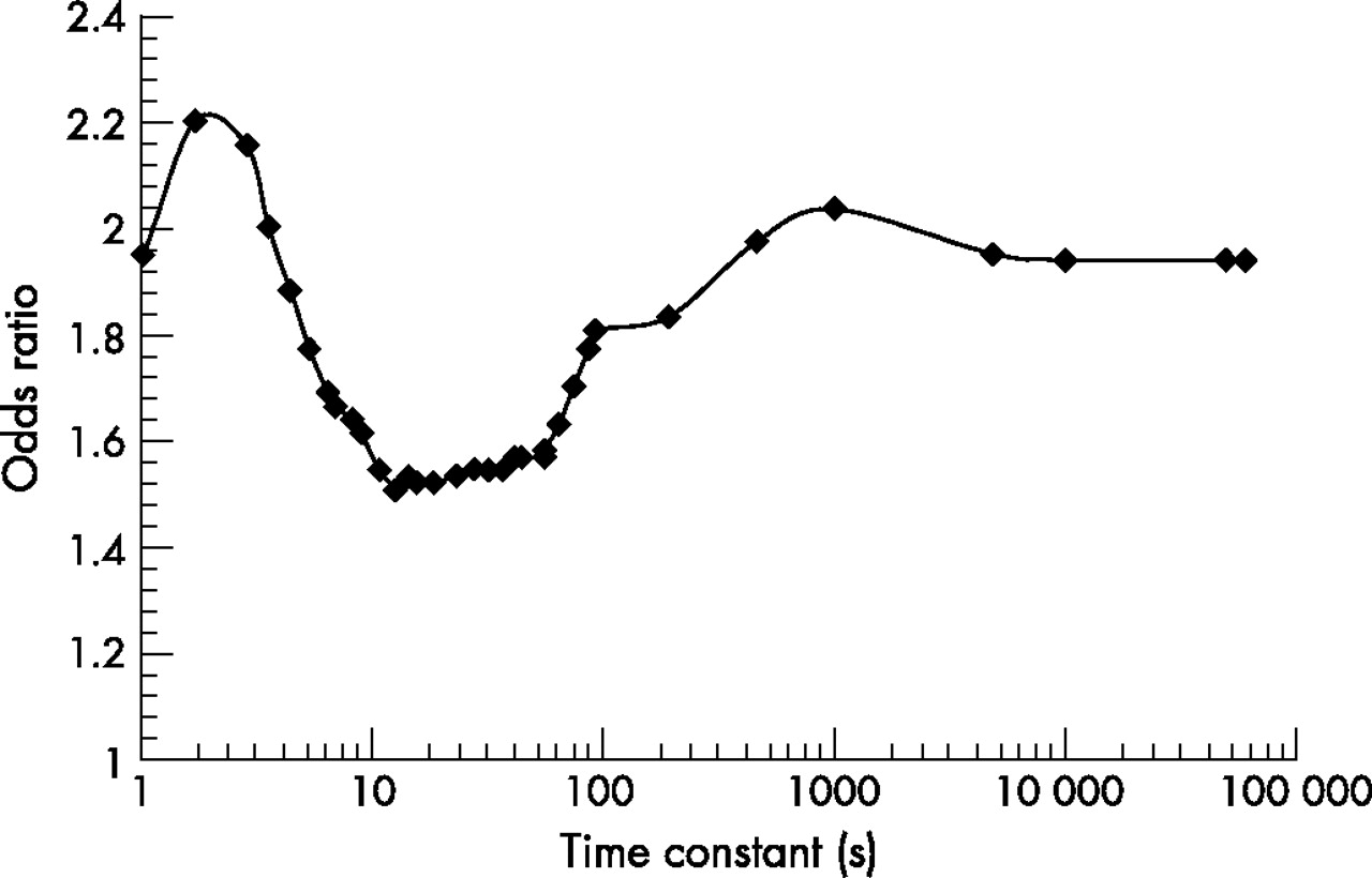
The model also allowed an investigation of alternative assumptions about the recovery time. This can be thought of as a kind of sensitivity analysis, and also as a way of using epidemiological data to provide information about a biological process, the recovery time following strain. For values of the recovery parameter τ, ranging from 1 to 100 000 seconds, the dose metric was calculated for each of the 68 participants, and then each resulting set of dosimetric data was fit to the case control data to calculate an odds ratio (fig 1). These odds ratios were then plotted against the varying values of τ to yield a continuous trend. The two peaks in this figure suggest that two very different physiologic processes are at work—one quite short (about 2 seconds) and the other on a much longer time scale (about 1000 seconds). Such information may be useful for improving understanding of pathophysiological mechanisms underlying repetitive strain injuries.

The preceding two examples illustrate models in which it was necessarily assumed that critical model parameters, such as clearance and physiological recovery times, were constant among all members of the population. It would be desirable to be able to relax this assumption, when data permit. The following example illustrates the use of data on individual risk modifiers to estimate dose metrics that will vary among cohort members with the same exposure experience.

A dosimetric model of dioxin exposure and lung cancer

A cohort study conducted by Fingerhut and colleagues found increased all-cause cancer as well as lung cancer mortality among workers at 12 US chemical plants where dioxin exposure occurred.³² Salvan and colleagues used serum TCDD (2, 3, 7, 8-tetradichlorodibenzo-p-dioxin) data collected at a single point in time on a subset of these workers, combined with occupational history data, to estimate a lifetime dioxin dose (part per trillion-years) for the members of this cohort.^33,34 It was hypothesised that body fat would be inversely proportional to bodily clearance of dioxin. The model had the form of a single compartment pharmacokinetic model assuming linear kinetics. Individual body mass index data were available for about 80% of the cohort, and were used to estimate per cent body fat and its rate of change over time among cohort members. The clearance parameter of the one compartment model was allowed to vary among individuals and within individuals over time, determined by time-dependent individual per cent body fat estimates. The investigators used the resulting individual serum TCDD dose estimates in a cohort mortality analysis to estimate the cancer rate ratios comparing those with doses based on only “background” dioxin exposure (assumed to be 7 parts per trillion-years) to those with doses up to 1000 times this level. The results suggest a strong association between dioxin dose and lung cancer, and because this analysis used serum TCDD doses and not simply the exposure data, the results may be more readily generalised to other populations for which serum doses were either measured directly, or estimated with a dosimetric model.

CHOOSING THE BEST EXPOSURE/DOSE METRIC

Epidemiological studies can be expensive and time-consuming, especially when a careful exposure assessment has been performed. When the time comes to analyse the data, it is hard to justify selecting just one measure of exposure or dose—in practice, several different measures are generally tested. How then, are we to choose among the various associations that result from this repeated analysis? What are the criteria for choosing the “best” measure of exposure?

First, the better indices will usually yield better statistical fits to the epidemiological data.³⁵ It is tempting to think that the better index will yield a stronger association with outcome (as in greater slope or higher relative risk), but this method has been shown to potentially lead to bias.³⁶ There is also the problem that different indices often have different scales, such that they cannot be directly compared. Goodness of fit will often be evaluated with a likelihood statistic, such as the −2-log likelihood, or the deviance. In linear models, an overall F statistic is preferable to the R² as a measure of fit, because the latter is quite sensitive to changes in extreme values. An additional problem is that if the exposure estimates derived from the various plausible models are strongly correlated with each other and/or are measured with significant misclassification, then an “inferior” model may show a better statistical fit than a “superior” model in a particular dataset. Thus, the decision as to which model is most appropriate to use should not be based solely on statistical performance.

In particular, there may be reasons to choose one exposure index or dose metric over another, even if it is not clearly superior in statistical performance. Ease of interpretation and comprehension may be additional considerations. Also, measures which are more easily generalisable across exposure settings are advantageous, if the objective is to make predictions about risk. A dose metric may be preferable to an exposure index if there are several routes of exposure, and one wants to estimate risk via all routes combined. Also, if one wants to be able to use the results to make predictions about risks resulting from quite varied exposures (different time patterns or routes), then a dose metric may be desirable.

A dosimetric model may provide an explicit method for considering interactions among different exposures. For example, Smith constructed a dosimetric model for silica and lung fibrosis which explicitly incorporated the effect of smoking on particle clearance from the airways.³⁷ This may be preferable to the standard approach of including smoking as an independent covariate in the epidemiological model.

CONCLUSIONS

Dosimetric modelling may be useful to improve the sensitivity of epidemiological models. However, it will never make up for deficiencies in the measurement of exposure; bad exposure data cannot be improved by estimating dose. Further, one must be careful that errors in exposure estimation are not hidden by feeding them into a dosimetric model, removing the risk analysis a further step from the raw exposure data. That said, there are several important motivations for dosimetric modelling. First, in some situations it may improve study validity and precision by weighting exposure data in a way that improves the fit of epidemiological models. This is especially likely to occur when studying non-linear exposure-risk relations, and may allow greater sensitivity in the detection of new, previously unidentified hazards. Epidemiologists can study exposures which confer fairly large risks without the need for dose modelling; even if the use of simple exposure measures introduces substantial misclassification, the risk may still be detectable. A second, related motivation is that dosimetric modelling may allow epidemiologists to investigate new mechanistic hypotheses formally in ways that are not possible with simple measures of exposure. Also, dosimetric models make it easier to extrapolate results, particularly when multiple routes of exposure are involved. Despite these potential advantages, dosimetric modelling should not be a substitute for conventional exposure–response analysis. It may be a logical next step, after the exposure data have been used to their fullest to quantify exposure–risk associations. At that point, dosimetric modelling may be useful for all of these reasons.

A serious deterrent to dosimetric modelling is the need for additional assumptions about the structure of the model, and the values of its parameters. It is important to remember, however, that if one chooses a simple summary measure of exposure, one is substituting implicit assumptions for explicit ones (about the proportionality between the exposure and dose, for example), and the same misclassification will result in either case if the assumptions are incorrect.

Dosimetric modelling has great potential for risk identification and dose–response characterisation. Further applications in occupational epidemiology should be encouraged where adequate exposure data are available.