


Abstract
One hundred and twenty-five new high-precision spectropolarimetric observations have been obtained with ESPaDOnS (Eschelle Spectro-Polarimetric Device for the Observation of Stars) at the Canada–France–Hawaii Telescope and Narval at Télescope Bernard Lyot to investigate the magnetic properties of the classical Be star ω Ori. No Stokes V signatures are detected in our polarimetric data. Measurements of the longitudinal magnetic field, with a median error bar of 30 G, and direct modelling of the mean least-squares deconvolved Stokes V profiles yield no evidence for a dipole magnetic field with polar surface strength greater than ∼80 G. We are therefore unable to confirm the presence of the magnetic field previously reported by Neiner et al. However, our spectroscopic data reveal the presence of periodic emission variability in H and He lines analogous to that reported by Neiner et al., considered as evidence of magnetically confined circumstellar plasma clouds. We revisit this hypothesis in light of the new magnetic analysis. Calculation of the magnetospheric Kepler radius RK and confinement parameter η* indicates that a surface dipole magnetic field with a polar strength larger than 63 G is sufficient to form of a centrifugally supported magnetosphere around ω Ori. Our data are not sufficiently sensitive to detect fields of this magnitude; we are therefore unable to confirm or falsify the magnetic cloud hypothesis. Based on our results, we examine three possible scenarios that could potentially explain the behaviour of ω Ori: (1) that no significant magnetic field is (or was) present in ω Ori, and that the observed phenomena have their origin in another mechanism or mechanisms than corotating clouds. We are, however, unable to identify one; (2) that ω Ori hosts an intermittent magnetic field produced by dynamo processes; however, no such process has been found so far to work in massive stars and especially to produce a dipolar field; and (3) that ω Ori hosts a stable, organized (fossil) magnetic field that is responsible for the observed phenomena, but with a strength that is below our current detection threshold. Of these three scenarios, we consider the second one (dynamo process) as highly unlikely, whereas the other two should be falsifiable with intense monitoring.
1 Introduction
Be stars are defined as non-supergiant B stars whose spectrum has, or has had at some time, one or more Balmer lines in emission (Collins 1987). More recently, the term ‘classical Be star’ has been introduced to exclude Herbig AeBe and Algol systems from the definition (e.g. Porter & Rivinius 2003).
Classical Be stars exhibit strongly variable winds evidenced by rapidly variable ultraviolet (UV) resonance lines of highly ionized species, as well as spectral and photometric variations on time-scales from hours to decades. Intermittently, these stars develop easily detectable, quasi-stationary circumstellar Keplerian discs, due to episodic ejections of mass called ‘outbursts’. Such discs are photoionized by radiation from the central star, and naturally produce strong recombination lines in emission, particularly lines of hydrogen and helium in the optical and infrared domains. The phases of emission are known as the ‘Be phenomenon’. The main changes in the emission line profiles reveal changes in the structure of the circumstellar envelope due to subsequent outbursts.
The ejections and consequently the existence of the flattened envelope are thought to be related to the typically high rotational velocities of Be stars. However, rotation by itself cannot explain the formation of the disc. Indeed, Be stars rotate on average at 88 per cent of the critical angular velocity in our Galaxy (Frémat et al. 2005), and significantly subcritical rotation speeds were found for early-type Be stars (Cranmer 2005). Huat et al. (2009) recently confirmed that outbursts are directly correlated to amplitude changes of the pulsation modes in Be stars and are therefore the probable provider of the additional angular momentum required to eject material from the surface of the star. However, Neiner et al. (in preparation) showed that the additional angular momentum probably arises from stochastically excited waves in the stellar convective regions rather than from a beating of κ-driven modes as suggested by Rivinius et al. (2001) for μ Cen. The presence of stochastic pulsation modes has indeed been recently confirmed in a hot Be star (Neiner et al. 2012b).
Historical searches for magnetic fields in Be stars have not led to the direct detection of magnetic fields (Barker et al. 1985; Silvester et al. 2009). In the last few years, claims of direct detections of magnetic fields in Be stars have been published (e.g. Yudin et al. 2012). However, these claims have been later shown to be spurious (e.g. Bagnulo et al. 2012). The general absence of fields in Be stars is supported by the MiMeS (Magnetism in Massive Stars) Survey (Grunhut et al. 2012), in which high-precision polarimetric observations of 43 Be stars yield no Zeeman detections. Consequently, as of today, there exists no firm direct detection of a magnetic field in any classical Be star.
ω Ori (HD 37490) is quite possibly the most compelling example of a classical Be star in which a magnetic field is suggested by indirect measurements. ω Ori is a well-studied rapidly rotating classical Be star with spectral type B2IIIe, Teff ∼ 20 000 K and log g ∼ 3.5. These parameters were determined from detailed spectral modelling by Neiner et al. (2002, 2003c, hereafter N03). In addition, Neiner et al. (2002) determined that the rotation axis inclination is i ∼ 35° but with a large uncertainty, while N03 determined the more precise value i = 42 ± 7°. Finally, Neiner et al. (2002) obtained a projected rotational velocity v sin i = 179 ± 4 km s−1 (while N03 found 172 km s−1 but with a less good uncertainty).
ω Ori is known to undergo multiperiodic short-term spectroscopic and photometric variations attributed to non-radial pulsations with P = 0.97 d and transient orbiting material (Neiner et al. 2002). In addition N03 found that UV resonance lines, sensitive to the stellar wind, as well as several optical quantities, in particular emission in hydrogen and helium lines, show variations with P ∼ 1.3 d, which was suggested to be the rotation period. In addition, their longitudinal magnetic field measurements (Bℓ) varied with a similar ∼1.3 d period. It was suggested by N03 that the Bℓ and wind variations were the result of the presence of a dipolar magnetic field with surface polar field strength Bd = 530 ± 230G and an obliquity angle between the magnetic axis and the rotational axis of β = 50 ± 26°. They proposed that the H and He emission variability resulted from corotating, magnetically confined clouds. However, although Bℓ values showed variability, no clear direct Stokes V signatures were observed with the instrumentation available at that time.
In this paper, we present an extensive spectropolarimetric monitoring of ω Ori obtained with the new generation of spectropolarimeters ESPaDOnS and Narval (Section 2), with the aim of confirming its magnetic field and better defining its properties. In Section 3, we discuss the observed long-term and short-term emission variability of ω Ori. We analyse the new spectropolarimetric data in Section 4, and re-analyse the data from N03 in Section 5. Finally, we discuss our results in Section 6.
2 Observations
High-resolution (R ∼ 68 000) circular polarization (Stokes V) spectra of ω Ori were obtained with the ESPaDOnS spectropolarimeter, mounted on the 3.6-m Canada–France–Hawaii Telescope (CFHT) in Hawaii, and the Narval spectropolarimeter, mounted on the 2-m Bernard Lyot Telescope (TBL) in France, as part of the commissioning ESPaDOnS runs (04BE80, 04BE37 and 04BD51), PI programmes (Neiner on Narval L062N05 and L072N08, and Landstreet on ESPaDOnS 07BC08) and of the MiMeS project (Wade on ESPaDOnS 08BP13). Six different epochs of spectropolarimetric data were obtained in 2004, 2007 January, 2007 November, 2008 January, 2008 October and 2009 January that resulted in 125 polarimetric observations. A log of the observations is provided in Table 1.
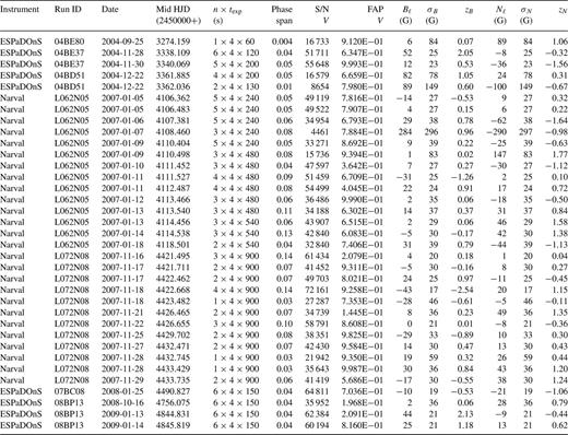
Magnetic measurements of ω Ori. Indicated are the instrument used, the run ID, the date of the observation, the heliocentric Julian date of mid exposure, the number of exposures and exposure time, the potential phase coverage assuming a period of 1.307 d, the mean S/N achieved in the LSD Stokes V profile, the false alarm probability (FAP) as measured from the observed Stokes V spectrum, the longitudinal field measurement obtained from Stokes V (Bℓ) and the diagnostic null (Nℓ) profiles, the uncertainty in these field measurements (σB and σN) and the significance of the measurements (zB = Bℓ/σB and zN = Nℓ/σN)
The ESPaDOnS and Narval twin instruments are optical echelle spectropolarimeters covering a wide wavelength range (3700 to 10 500 Å). A complete polarization observation consists of four individual subexposures between which the half-wave Fresnel rhombs are aligned in different orientations in order to remove first-order systematic errors in the polarization analysis. The extraction of the ESPaDOnS and Narval spectra, along with wavelength calibration, was accomplished using libre-esprit (Donati et al. 1997), a dedicated automatic reduction package installed at both CFHT and TBL. All spectra were normalized using a fifth-order polynomial (or lower) fit to each individual order. The final reduced products consist of an unpolarized Stokes I and a circularly polarized Stokes V spectrum. A diagnostic null N spectrum that is used to test for spurious signals in the data is also created by combining the individual subexposures in such a way that the polarization should cancel out. The mean signal-to-noise (S/N) of the data per 1.8 km s−1 pixel is ∼1250.
3 Spectral and Emission Variations
3.1 Long-term disc evolution and outbursts
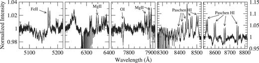
ω Ori is a Be star for which emission is known to significantly vary from one epoch to another, changing from B phases to Be phases (Hubert-Delplace & Hubert 1979). The star shows recurrent small outbursts every 11 months (Bergin et al. 1989; McDavid et al. 1996) in addition to the few major outbursts that have also been observed, e.g. in 1992, as indicated by the Hα maximum intensity enhancement, as shown in Fig. 1. During the observations presented here, another major outburst occurred at the end of 2004 and, for the first time, lines of several ions such as Fe ii were also observed in emission, as exhibited in Fig. 2. Another relatively strong outburst occurred in 2008 and enhanced emission can also be seen in our 2008 observations.
![Evolution of the maximum emission intensity for Hα. Data used in this plot also include the spectra presented by Neiner et al. (2002) and spectra available from the BeSS data base [BeSS (Be Star Spectra) is a data base collecting spectra of all known Be stars, available at http://basebe.obspm.fr (Neiner et al. 2011).] The epochs of ESPaDOnS and Narval observations are indicated with red diamonds. The time when emission is present in Fe ii lines is indicated. A thin solid line is provided for display purposes.](https://oup.silverchair-cdn.com/oup/backfile/Content_public/Journal/mnras/426/4/10.1111/j.1365-2966.2012.21833.x/2/m_426-4-2738-fig001.jpeg?Expires=1716411622&Signature=oZKRYIyuwaQElB-uFHAaUIdi8fwH~v6sPvT4Nbc~pEVpQIwoYr3PH0mOgutQusvts5rRhOFvuirNGphEHrUD9wWktUSVMO4n98iFvF29gSphQJcBKOz3S55ktT4anEx8Q~uQtZnaWISLFgbmfmk8ESBogUOOqoVic0uc~~rsw59QLGyOD5X~F9SuFjaHy4ZehYN1dX-mY0IT1x5-BzJz62XPMz1kjfuI7FK319p8xRDLULHmS4xAVU6wJALITm0WrQswctNl93uptT-jaj02H-zJARpQUPqb-PlKspqSAnkYrJmmh~m4QVrU8~Q62uPNjWXod1Hgytcu2sXZv7d~8g__&Key-Pair-Id=APKAIE5G5CRDK6RD3PGA)
Evolution of the maximum emission intensity for Hα. Data used in this plot also include the spectra presented by Neiner et al. (2002) and spectra available from the BeSS data base [BeSS (Be Star Spectra) is a data base collecting spectra of all known Be stars, available at http://basebe.obspm.fr (Neiner et al. 2011).] The epochs of ESPaDOnS and Narval observations are indicated with red diamonds. The time when emission is present in Fe ii lines is indicated. A thin solid line is provided for display purposes.
Example of lines that were observed in emission in the spectrum of ω Ori obtained on 2004 September 25 with ESPaDOnS during a major outburst. Examples of Fe ii, Mg ii, O i emission lines as well as hydrogen lines of the Paschen series are labelled.
3.2 Short-term spectral variations
3.2.1 Known frequencies
Short-term variations in line profiles of ω Ori have been detected (e.g. Neiner et al. 2002) and attributed to non-radial pulsations. The main pulsation frequency is ƒpuls = 1.03 c d−1 (Ppuls = 0.97 d) and corresponds to an l = 2 or 3 and |m| = 2 pulsation mode.
Transient frequencies have also been detected and attributed to orbiting material due to the recurrent ejections of material from the star.
The rotation frequency of ω Ori was estimated to be ƒrot = 0.73 d−1 (Prot = 1.37 d) by Neiner et al. (2002). N03 found variations in the equivalent widths of UV resonance lines sensitive to the wind with the frequency ƒwind = 0.777 d−1 (Pwind = 1.286 d) and, assuming that the wind is rotationally modulated, proposed this to be a more precise determination of the rotation frequency. In addition, N03 found that spectropolarimetric quantities, as measured from MuSiCoS (Multi-site Continuous Spectroscopy) spectra, also varied with a similar period PB = 1.29 d, and that emission quantities varied with twice the frequency ƒem = 0.765 d−1 (half of Pem = 1.307 d). Therefore, N03 concluded that the rotation period is Prot ∼ 1.3 d.
3.2.2 Variation of spectral quantities with rotation
The new data presented here have not been acquired with a sampling rate that allows for the precise investigation of short-term variations. It is however possible to measure spectral quantities and fold them with known periods to evaluate their presence in the data.
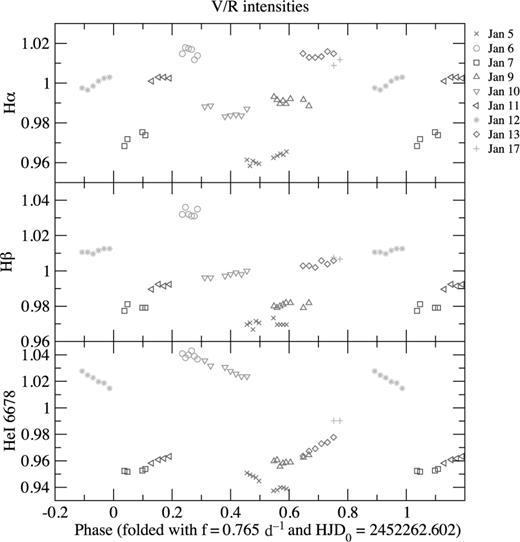
Fig. 3 shows the variation of the violet (V) over red (R) peak intensities for the Hα, Hβ and He i 6678 Å lines observed in 2007 January, folded with the period P = 1.37 d (ƒ = 0.765 c d−1) as proposed by N03 from their analysis of the same quantities. The He i 6678 Å data appear to coherently phase with this frequency, and we therefore infer that this frequency is present in the 2007 January data. We also find it in the 2007 November data. Coherent variations in Hα and Hβ are also clearly present when phased with this frequency, but with a different shape. The sawtooth shape of the variations visible for the He i 6678 Å line likely indicates that the material emitting in the He i line is closer to the star than the Hα emitting material and undergoes occultation by the star.
Variations of the V (violet) over R (red) peak intensities for various lines observed in 2007 January, folded with the rotation frequency ƒ = 0.765 d−1 as determined in N03. Colour/symbol coding is used for each night of observations.
The variations observed in 2007 indicate that the circumstellar emission is consistent with the results found by N03. Both data sets (in 2007 and in N03) correspond to epochs of low emission. However, we could not detect these variations in the 2004–2005 data, nor in the most recent 2008 data, when the emission was strong.
V/R emission variations in Be stars are attributed to overdensities in the circumstellar environment. The fact that these overdensities vary with the rotation period, and with two maxima per period, was interpreted by N03 as evidence for two corotating clouds located on opposite sides of the star.
4 Magnetic Field Analysis
4.1 Least-squares deconvolution analysis
Before analysing the spectropolarimetric observations, multiple spectra were combined to increase the S/N of our observations. The number of spectra combined per night was chosen not only to maximize the S/N, but also to limit the total phase spanned by the binned observations to ≲0.15 cycles and to reduce the smearing of any potential Zeeman signature. In imposing this criterion, we have assumed the P ∼ 1.3 d rotational period proposed by N03. The properties of the combined spectra are presented in Table 1. The exposure times listed in Table 1 indicate the total exposure time of the combined observations, but since some of the sequences of combined observations were not obtained consecutively, we also list the total phase spanned by each sequence of observations.
In order to improve our ability to detect weak Zeeman signatures, we applied the least-squares deconvolution (LSD) procedure of Donati et al. (1997) to the combined spectra. The line mask (which contains information about the line rest central wavelength, predicted line depth and measured Landé factor) was extracted from the Vienna Atomic Line Database (Piskunov et al. 1995) for a Teff = 20 000 K and log g = 3.5 atmosphere model, covering the full spectral range from 3700 to 10 500 Å. When measured Landé factors were unavailable they were computed from L-S coupling. This list resulted in 2672 helium and metal lines. However, this list also included lines that were blended with hydrogen lines (which are not included in the LSD procedure) and telluric bands as well as lines that are often observed to be in emission. The inclusion of these lines diminishes the agreement between the observed spectra and the LSD modelled unpolarized spectra (obtained from the convolution of the line mask and LSD I profile). We therefore proceeded to remove all lines blended with hydrogen or telluric regions and limited the line list to include only lines with intrinsic line depths greater than 10 per cent of the continuum (to reduce the contribution from weak lines that are invisible in our spectra). Lastly, we removed all lines that showed any emission in any of our post-2004 era spectra, resulting in 328 lines remaining in our adopted mask. As a last step, we also interactively adjusted the depth of each line in our mask to improve the quality of the fit between the observed spectra and the LSD modelled spectrum. This method has been tested on several magnetic stars: the results from these analyses suggest that the agreement between the LSD V model and the observed spectrum improves when the agreement with the LSD I model improves (Grunhut et al., in preparation). However, this makes the basic assumption that depths of the observed unpolarized spectral lines are inconsistent with the line mask due to incorrect data in the line mask (e.g. non-solar abundances, NLTE (Non-Local Thermodynamic Equilibrium) effects or incorrect atomic data), or is a result of continuum emission that would affect the polarized light in a similar fashion as the unpolarized light. This assumption may not be correct in Be stars as the line emission may affect the unpolarized light but not necessarily the circularly polarized light. In any event we conducted our analysis using several variations of this adopted mask, some of which did not include the modified line depths or removed lines. All LSD profiles were computed on a spectral grid with a velocity bin of 10.8 km s−1.
According to the detection criteria of Donati et al. (1997), none of our LSD profiles yield a significant detection of Stokes V signal (i.e. FAP <10−3). We therefore conclude that the new polarimetric data provide no direct evidence for the presence of a magnetic field in ω Ori.
4.2 Analysis of the longitudinal magnetic field
Following the procedure of N03, we proceeded to measure the longitudinal magnetic field (Bℓ). The Bℓ measurements and equivalent measurements Nℓ extracted from the diagnostic null were computed for each LSD profile in a manner similar to that described by Silvester et al. (2009), using an integration range from −197 to 197 km s−1 about the centre of gravity of the LSD I profile, consistent with the method used by N03. The Bℓ measurements range from −100 to 90 G, with a typical uncertainty of σ ≃ 30 G. All of the measurements are consistent with a null longitudinal magnetic field (i.e. |Bℓ| < 3σ B). LSD profiles extracted using variations of our adopted line mask yield longitudinal field measurements consistent within their error bars with those obtained using the adopted mask. The longitudinal field and null measurements from each of the combined polarimetric observations, the mean S/N of the LSD Stokes V profiles and the FAPs measured from the LSD profiles extracted using the adopted mask are listed in Table 1.
4.2.1 Period search
A period search was performed on the Bℓ measurements using the clean-ng algorithm (based on Högbom 1974; Roberts, Lehar & Dreher 1987, see also Gutiérrez-Soto et al. 2009). The cleaned periodogram contains about a dozen periods, the strongest of which is located at about 0.66 d. The only period near 1.3 d is located at 1.275 d; however, this is only the eighth most significant period in the periodogram, with a power corresponding to just 3.5 per cent that of the most significant period. Our strongest period 0.66 d, however, is about one-half 1.3 d. This half-period was also found by N03 as the dominating period in the emission quantities.
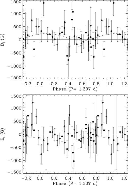
However, phasing the Bℓ measurements according to any of these periods yields no coherent variation (see e.g. Fig. 4), and fitting the resultant variations with sinusoids yields reduced χ2 values that are comparable to a straight-line fit to the data and similar to the reduced χ2 values achieved using many other periods in the range 0.1–5 d.
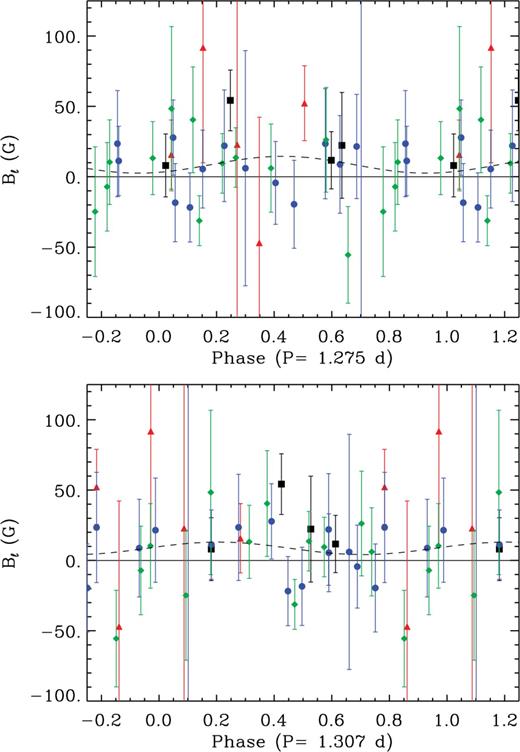
Bℓ measurements from different epochs of observation phased with our period of 1.275 d (top panel) and the period P = 1.307 d of N03 (bottom panel). Included are the measurements with ESPaDOnS from 2004 (red triangles), Narval from 2007 January (blue circles), Narval from 2007 November (green diamonds) and ESPaDOnS from 2007–2009 (black squares). Also shown are a best-fitting sinusoidal curve to the entire data set (dashed curve) and a line representing a null-field model (solid curve). The error bars represent the 1σ uncertainties. Note the similar lack of coherent phasing with either period.
Since we are unable to significantly confirm the period reported by N03 in our current data set, we adopted their period P = 1.307 d, as inferred from their analysis of the emission quantities, as the rotation period for the following analysis. In the bottom panel of Fig. 4 we show the Bℓ measurements phased with this period. The phased measurements appear qualitatively similar to those phased with our 1.275 d period, as illustrated in Fig. 4 (top panel), with no clear pattern to the variability and a comparable reduced χ2.
However, the imprecision of the adopted period (±0.1 d) introduces significant phase offsets between data sets separated by long periods of time, making it impossible to correctly phase all of our data obtained at different epochs. We therefore continued our analysis by only attempting to phase Bℓ measurements of individual data sets. We choose the two Narval data sets for which enough measurements are available to carry out sinusoidal fits to the data and therefore determine potential phase offsets. The sinusoidal fits to the data (included in Fig. 5) illustrate the potential phase offset between the two data sets (ϕ0 = −0.10 ± 0.18 for the 2007 January data set and ϕ0 = 0.70 ± 0.36 for the 2007 November data set) when using the HJD0 of N03 and ϕ0 as the phase of maximum positive Bℓ.
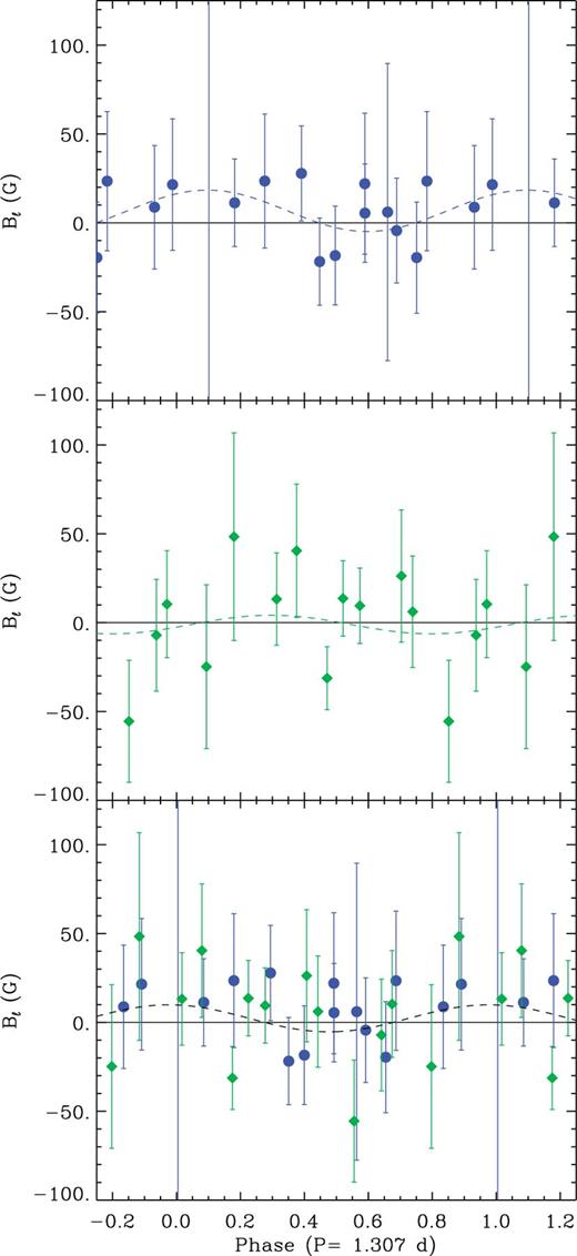
Bℓ measurements from the 2007 January (top) and 2007 November (middle) Narval data sets, phased with P = 1.307 d. Also included are sinusoidal fits to the individual data sets (dashed curve) and a line representing a null-field model (solid line). The bottom panel shows the same two data sets but phase-corrected such that phase 0.0 occurs at maximum positive Bℓ.
After correcting the two individual data sets to a common ϕ0 = 0, we computed a new best-fitting sinusoid to the combined data sets (as illustrated in the bottom panel of Fig. 5). The results of our best fit and of a null-field model indicate a reduced χ2 = 0.58 and 0.54, respectively, indicating that the two models are equivalent. In addition, analogous analysis using the diagnostic null Nℓ measurements provides similar results. We note that the value of the reduced χ2 are somewhat low, suggesting that σ uncertainties may be overestimated. This will be discussed below (Section 4.3.1).
4.2.2 Dipole field upper limit
To investigate the upper limits on the possible magnetic field of ω Ori, we assume that the field can be described by the dipole oblique rotator model (ORM), as was also done by N03. This model is characterized by four parameters: the phase of closest approach of the positive magnetic pole to the line of sight ϕ0, the inclination i of the stellar rotation axis to our line of sight, the obliquity angle β between the magnetic axis and the rotation axis and the dipole polar surface field strength Bd. We modelled the phased Narval longitudinal field measurements discussed in Section 4.2.1 by comparing the observations to longitudinal field curves computed for a grid of Bd and β values. We adopted i = 42 ± 7° and a limb darkening coefficient of 0.4, as employed by N03 in their analysis. The phase of closest approach ϕ0 was left as a free parameter and determined by least squares. The values of the reduced χ2 as a function of Bd and β that characterize this comparison are illustrated in Fig. 6.
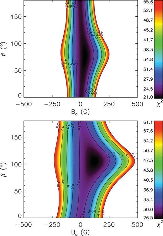
χ2 landscape as a function of the dipole field strength Bd and obliquity angle β for an inclination of i = 42° as measured from the Bℓ measurements using our adopted mask (top) and the mask of N03 (bottom). A colour version of this figure is available online.
Our results indicate that the inferred surface dipole field strength Bd is consistent with a null-field model (Bd = 40 ± 110 G, for 1σ limits) and β is unconstrained (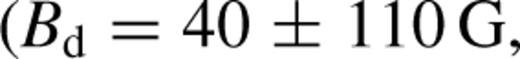 ) for i = 42 ± 7°. The 3σ contour places an upper limit of 180 G on the dipole strength Bd. This result is formally inconsistent with the field reported by N03 (
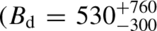 G). Analogous modelling of the Nℓ measurements results in a best fit
  G and
G and  . Therefore, the Bℓ and Nℓ measurements yield consistent results for Bd and Nd with compatible uncertainties.
To better understand the relationship between these results and those of N03, we calculated a second set of LSD profiles and Bℓ measurements using the line mask of N03 and re-performed the analysis described above. This mask differs from our adopted mask in that it contains fewer (80) lines, distributed over a more limited (4510–6580 Å) wavelength range (corresponding to the bandpass of the MuSiCoS instrument). The χ2 landscape using the N03 mask favours a model with a best fit  G and
G and  (see the bottom panel of Fig. 6). Although the value of Bd is higher than with our adopted mask, it is still consistent with a null-field model.
4.3 Analysis of the Stokes V profiles
4.3.1 Detectability of the magnetic signal
To further constrain the magnetic field characteristics, we proceeded to analyse the LSD Stokes V profiles extracted from the Narval spectra.
We first compared the observed LSD Stokes V profiles to synthetic profiles computed assuming the rotational period and the magnetic configuration reported by N03 (Bd = 530 G, β = 50°), as shown in Fig. 7. The model profiles are computed by performing a disc integration of local Stokes V profiles, assuming the weak field approximation (Landstreet 2009). The characteristics of the LSD I profiles were chosen to provide the best fit to the individual observed LSD I profiles, but do not take into account asymmetries in the observed line profiles. In particular, we adopted v sin i = 179 km s−1 and varied the line depth to best match the mean Stokes I LSD profile. The wavelength and Landé factor of the line corresponded to the scaling factors of the lines in the line mask. We adopted ϕ0 determined from the sinusoidal fits to the Bℓ measurements of the individual Narval runs to provide the most consistency with the N03 model.
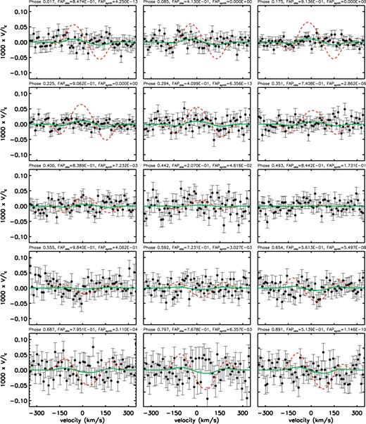
Comparison of a select number of the observed Narval Stokes V profiles (black circles) compared with the synthetic Stokes V profiles (dashed red and solid green lines) corresponding, respectively, to the parameters given in N03 at the indicated rotational phase and to the same parameters but Bd = 90 G. Included for each profile is the FAP, calculated for both the observed and synthetic profiles for the red curves. A FAP between 10−5 and 10−3 indicates a marginal detection and <10−5 indicates a definite detection. Note that the synthetic profiles following N03 (dashed red curves) would result in the detection of a magnetic signature at several phases, while no signal is ever detected in our observations. In contrast a field with Bd = 90 G (solid green curves) would not be detected.
As illustrated in Fig. 7, we find significant disagreements between the N03 model (red curves) and the Narval observations (black dots). We can quantify this by comparing the FAP as computed from the observations with the FAP computed from the N03 model profiles, to which we have added random Gaussian noise corresponding to the mean S/N of the real observations. These FAP values are indicated in Fig. 7. According to these results, our observations should have resulted in the detection of a significant signal in Stokes V for 60 per cent of our observations if a field with the parameters inferred by N03 were present.
To further quantify this point, we compared the cumulative distribution of FAPs as derived from our observations and synthetic models, as presented in Fig. 8. The cumulative distributions were derived from FAPs obtained from 100 different variations of the random noise for each model. In Fig. 8, we compare the Stokes V distribution (solid black) to distributions computed using different magnetic field strengths and the geometry proposed by N03. We find that a Bd = 90 G polar field strength (double dot–dashed magenta curve) presents the best fit to the Stokes V distribution. A two-sided Kolmogorov–Smirnov test indicates that the hypothesis that the null field and the observed Stokes V FAP curves are derived from the same distribution is not ruled out with 15.1 per cent probability, while the hypothesis that a 90 G field and the observed Stokes V FAP curves are derived from the same distribution is not ruled out with 84.1 per cent probability.
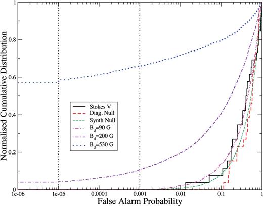
Cumulative distribution of FAPs. Distributions are derived from the FAP as measured from the diagnostic null profiles (thick dashed red), the Stokes V profiles (solid black), synthetic null N profiles (thin dashed green), synthetic Stokes V profiles with Bd = 90 G (double dot–dashed magenta), Bd = 200 G (dash–dotted violet) and Bd = 530 G (dotted blue, corresponding to the model of N03). Also included are the vertical lines corresponding to the threshold for a definite detection (FAP < 10−5) and a marginal detection (10−5 < FAP < 10−3).
Using a field of Bd = 90 G for the models shown in Fig. 7 (green curves) rather than Bd = 530 G as suggested by N03 (red curves), we indeed find that the signatures in Stokes V become indistinguishable from the noise.
4.3.2 Bayesian analysis
As a final approach we analysed all the new LSD profiles using the Bayesian statistical method of Petit & Wade (2012). One limitation to all of the analyses performed in Sections 4.2.2–4.3.1 is that they implicitly assumed a phasing of the measurements with the 1.307 d period of N03. The Petit & Wade (2012) approach has the implicit advantage that it makes no assumptions about the phasing of the data, allowing us to use all of our new spectropolarimetric measurements. In addition, this approach inherently addresses issues arising from the imprecise period, the uncertain inclination and the potentially overestimated Stokes V uncertainties in the modelled profiles. The method compares each individual observation to a large grid of synthetic ORM Stokes V profiles corresponding to a particular (Bd, β, i) configuration, as well as all possible rotational phases ϕ of the observation. The parameters of the modelled Stokes I profile were chosen to provide the best overall fit to the average LSD I profile of our full data set; in particular, we used v sin i = 185 km s−1 (which is close to the v sin i = 179 km s−1 used above and taken from Neiner et al. 2002). We assumed that only ϕ can change between different observations, and we searched for the goodness of fit of a given (Bd, i, β) magnetic configuration using the overall best posterior probability density as computed from all observed Stokes V profiles using Bayesian inference techniques.
As described by Petit & Wade (2012), the ‘odds ratio’ compares the relative overall likelihood of two models: in this case, the null-field model, and a magnetic model in which the field is described by an oblique dipole configuration. The computed odds ratios for all the individual observations are in favour of the null-field model, with a few exceptions where both the null-field model and magnetic dipole models are equally likely. This is not sufficient to justify the use of the ORM model. Furthermore, although some individual observations can be fitted slightly better with a dipole model, these deviations cannot be attributed to a single dipole geometry when all the observations are considered together. Finally, considering all of the observations together, the odds ratio is a factor of 2 in favour of the non-magnetic model. Therefore, the odds ratio analysis does not provide evidence for the presence of a dipole magnetic signal in these observations.
The posterior probability density derived from our analysis (shown in Fig. 9) can provide an estimate of the dipole field strength admissible by our data set. As explained by Petit & Wade (2012) and illustrated in Fig. 6, no meaningful constraints can be put on the geometry angles i and β in the case of a non-detection. We can however place strong constraints on the allowed dipole field strength Bd. Within the 68.3, 95.4 and 99.7 per cent credible regions, we compute allowed upper limits of 32 G, 80 G and 283 G, respectively, for Bd from the Stokes V profiles. According to Petit & Wade (2012), a field near the 95.4 per cent limit (80 G) should in general have been detected with our current data set; however, a weaker field could remain undetected. This is consistent with the detectability limit at 90 G obtained from the cumulative FAP distribution in Section 4.3.1. The limit obtained with the Bayesian method (80 G) is slightly different than the one obtained with the FAP analysis, because we use all of the high-resolution data rather than just the Narval data sets.
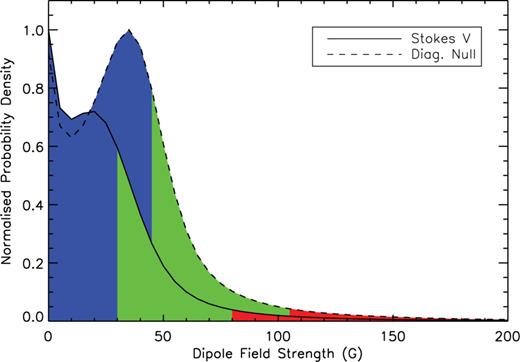
Marginalized probability density functions (PDFs) for the dipole field strength derived from our Bayesian analysis of the LSD profiles of all the high-resolution spectra. The PDFs have been normalized by their peak values in order to facilitate graphical representation. The parameter evaluation for the dipole model treats any difference with the model as additional Gaussian noise that is marginalized, leading to the most conservative estimate of the parameters. Three detection confidence regions (at 68.3, 95.4 and 99.7 per cent) are indicated in grey-scale (or colours in the online version).
The probability density distribution shown in Fig. 9 peaks at 0 G. However, the distribution is not monotonic: a second peak is observed at about 20 G. This peak is probably not related to the presence of a magnetic field, since the analogous probability distribution derived from the diagnostic null N profiles (also shown in Fig. 9) shows a similar structure at about 35 G. A close examination of individual and combined likelihoods and the marginalized posterior probability distribution shows that this feature is not produced by the fit to a single or small number of the LSD profiles, i.e. it is representative of the entire data set. For the moment, we are not able to identify its source, although we propose that it may be related to very weak spurious signatures in the V and N profiles caused by the star's line profile variability related to non-radial pulsations.
In the end, we conclude that our observations allow us to place a firm upper limit of 80 G on the polar field strength of any dipole magnetic field present in the photosphere of ω Ori. Larger polar field values are only admissible for aligned geometries with large i angle, which are unlikely.
5 Re-Analysis of the Musicos Data Set
Given that our new results do not recover the magnetic field proposed by N03, we decided to re-analyse the N03 MuSiCoS spectra. This was accomplished through the re-analysis of the original MuSiCoS LSD profiles calculated by N03, as well as computation of new LSD profiles that were calculated after re-reduction of the original MuSiCoS raw data with the newest version of esprit. In agreement with N03, we find that none of the MuSiCoS LSD Stokes V profiles results in a detection of significant signal. We then measured the longitudinal fields Bℓ and Nℓ from both sets of MuSiCoS LSD profiles in the manner described above. We find Bℓ and Nℓ values that are fully consistent with those of N03 but with slight differences, mainly due to the slightly different weighting of the lines in the LSD profiles and normalization. None of the MuSiCoS Bℓ measurements is significant at more than 3σ, and only one measurement is significant at greater than 2σ. See Fig. 10.
Phased Bℓ measurements of the MuSiCoS observations, with sinusoidal fits to each data set (dashed line) and a zero-field model (solid line). The top panel represents the Bℓ variations obtained with the mask of N03 (and is thus similar to Fig. 11 of N03), while the bottom panel represents the Nℓ measurements using this same mask.
We first attempted to confirm the periodicity of the Bℓ measurements discussed by N03. Using the clean-ng algorithm we were unable to detect any significant period near 1.3 d in the Bℓ measurements. However, a Lomb–Scargle periodogram of the Bℓ measurements does show signal about 1.307 d, and this period does not appear to be associated with the window function and is not present in the Nℓ measurements, supporting the results of N03. A sine fit with this period is shown in Fig. 10. On the other hand, this does not represent a global χ2 minimum, nor does it constitute the significant improvement in quality of fit (according to Gaussian statistics) that would characterize the formal detection of variability.
Finally, we derived the constraints on the ORM parameters using the same procedure as discussed above, phasing the measurements using the period of N03. Our re-analysis of the original MuSiCoS LSD profiles used by N03 results in a best-fitting model  G with
  (see Fig. 11). The results from the re-calculated MuSiCoS LSD profiles are consistent with these results, with a best fit
  G and
G and  . These results are consistent with the ones obtained by N03 (
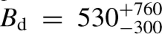 G and
G and 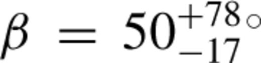 ), but also with a null-field hypothesis to within ∼1.2σ. The diagnostic null Nℓ results for the MuSiCoS data are fully consistent with a null field, as illustrated in the bottom panel of Fig. 11.
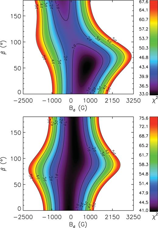
χ2 landscape as a function of the dipole field strength Bd and obliquity angle β for an inclination of i = 42° as measured from the Bℓ measurements of the MuSiCoS spectra (top) and the Nℓ measurements using the mask presented by N03. A colour version of this figure is available online.
6 Discussion
6.1 Magnetic confinement
Models of centrifugal magnetospheres (CM; Townsend & Owocki 2005) or dynamical magnetospheres (DM; ud-Doula, Owocki & Townsend 2008; Sundqvist et al. 2012) have been developed in the last decade to explain the rotational modulation of several observed quantities (such as Hα emission or X-ray emission) in magnetic massive stars (Petit et al. 2011). The details of the confinement depend on the interplay between radiative, magnetic and Coriolis forces. Most importantly, the magnetic confinement parameter, 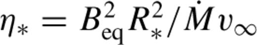 (ud-Doula & Owocki 2002), provides a relationship between these forces and the limits of this parameter dictate whether wind plasma can or cannot be magnetically confined above the stellar surface: if η* > 1 material is confined at the top of magnetic loops in the circumstellar environment, whereas if η* < 1 material is not confined. The location of the Alfvén radius RA with respect to the corotating Kepler radius RK provides the distinction between where the circumstellar plasma can be rotationally supported: if RA > RK, the plasma is centrifugally supported and the material is trapped above RK out to RA (i.e. there is a CM), whereas if RK > RA the transient suspension of trapped material establishes a DM below RA.
We computed η − *, R − A and R − K for ω Ori using the terminal wind velocity V − ∞ = 60O km −I, as inferred from the IUE) spectra of ω Ori, a typical mass-loss rate for Be stars  yr−lt)he, projected velocity vsin i = 179 km −1a nd the inclination i = 42° from Neiner et al. (2002) and Neiner et al. (2003a) respectively. We approximated the magnetic equatorial radius by the averaged stellar radius R − ⋆ = 5.9 R − ⊙ inferred from the rotation period,considering the probably high obliquityof the dipole and the stellar flattening of the star. With the upper limit of the magnetic fielddetermined from our Bayesian analysis B − d = 80LG, we find η − * = 7, R − A = 1.6 R − ⋆ and R − K = 1.4 R − ⋆ (note that these values neglect the uncertainties of the stellar parameters). Therefore, magnetic confinement of the circumstellar matter is possible: actually we only require 8 − d > 32 G for η − * > I, but in the case of a DM the emission measure would be very low and probably not detectable. A CM could exist if R − A > R − K i.e. for B − d) > 63 G. However, the confinement is not especially strong (for example, for σ”ori, η − * goes up to ∼106; for pulsating early B stars, such as βSNCep or ζ Cas, η − * ∼ 200) and the small difference between R − A and R − K implies a relatively small magnetosphere.
Fig. 12 shows a sketch of the possible centrifugally supported magnetosphere and circumstellar clouds, close to the star. The Keplerian disc is further out than the magnetosphere and, consequently, the magnetic field would have no significant impact on the Keplerian disc itself. Indeed the field energy B2 falls off as 1/r6, i.e. faster than the wind energy (typically 1/r4 far from the star) and, at the distance of the Keplerian disc (2R* just after a major outburst but 8R* during quiescent epochs), it is weak enough that it does not dynamically affect the disc.
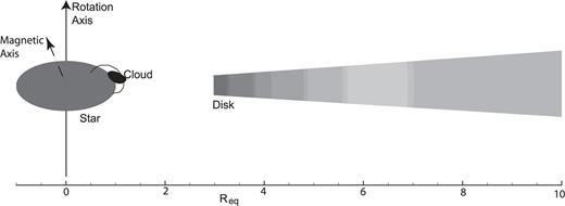
Sketch of ω Ori showing the Keplerian disc as well as one of the magnetically confined clouds close to the star (the other cloud is behind the star in this configuration). We used β = 76° in this sketch following Section 4.2; however, we caution that β is loosely constrained in our analysis, in particular N03 found β = 50°. As the star rotates, the magnetic axis precesses around the rotation axis and the two clouds pass in the line of sight of the observer.
6.2 Polarimetric and spectroscopic results
Observations of ω Ori suggest this star to be among a select few classical Be stars that show evidence of both a Keplerian disc and rotationally modulated circumstellar emission (see e.g. Porter & Rivinius 2003 for a review). ud-Doula & Owocki (2002) have already shown that the magnetically torqued discs produced from their simulations are inconsistent with observations of the discs of classical Be stars, and therefore it is not likely that the Be phenomenon is a result of large-scale magnetic confinement of the stellar wind. As evidenced by observations of the circumstellar emission (as well as the rotational modulation of wind sensitive lines in the UV, see N03) and our previous discussion that a weak surface field is capable of magnetically confining the wind plasma, it is therefore possible that ω Ori hosts both magnetically confined clouds close to the star and an extended Keplerian disc further out. In the next subsections, we examine each possible scenarios to explain the observations of ω Ori.
6.2.1 Scenario 1: ω Ori does not host a simple, large-scale magnetic field
The new spectropolarimetric data presented here are of higher resolution and higher S/N than those obtained with MuSiCoS by N03. However, the data still do not allow us to directly detect the presence of a Stokes V signature in the lines of ω Ori, even when using the LSD technique. The results presented in this study contradict the dipole magnetic field strength inferred by N03, and our likely upper limit of Bd ∼ 80 G implies that the N03 model overestimated the field strength by at least 150 G. Modelling of the Stokes V signatures, as expected from the N03 dipole field model, shows that excess signal in Stokes V should have been detected with ESPaDOnS and Narval with the S/N that we have obtained. Since these signatures are not detected, we conclude that a field with  G as proposed by N03 is not present at the surface of this star. It seems that weak fields have been systematically misestimated from the noisy MuSiCoS observations, as shown e.g. by the confirmation of the measurement of a magnetic field in V2052 Oph with Narval data with Bd ∼ 400 G (Neiner et al. 2012a) rather than the 250 G found with MuSiCoS (Neiner et al. 2003b), or that of ζ Cas with Bd = 56 G from Narval data (Briquet et al., in preparation) compared to the 335 G from MuSiCoS (Neiner et al. 2003a).
Nevertheless, a Bayesian analysis of the Stokes V profiles suggests that a dipole magnetic field with Bd < 283 G is possible, and Bd < 80 G is even more likely. Larger field strengths would require geometries with large i angles, which are unlikely according to the results of spectral modelling by Neiner et al. (2002). In addition, the S/N of our Stokes V measurements consistently suggests that it is likely that Bd < 90 G, i.e. that profiles with field strengths less than 90 G would not be detectable in the new data. Therefore, we cannot rule out the presence of a weak magnetic field in ω Ori.
A non-magnetic result for ω Ori is completely in line with the results of the MiMeS survey of other Be stars – no magnetic field has currently been directly detected for any star within a sample of 43 massive Be stars, compared to a 6.5 per cent incidence rate among other B-type stars (Grunhut et al. 2012). However, one cannot rule out very weak magnetic fields for this larger sample of Be stars either. We are only capable of placing upper limits on the admissible dipole field strength, which can only be decreased with higher S/N data obtained during quiescent Be phases. Indeed, measuring a magnetic field in Be stars is particularly challenging due to the presence of the Keplerian disc and the occurrence of outbursts, notwithstanding the rapid stellar rotation.
Increasing the exposure time of spectropolarimetric measurements much above our maximum exposure time of 4 × 900 s (1 h) is not an option to try to detect a magnetic signature in the Stokes V profiles of ω Ori, as its pulsation period is 0.97 d (∼23 h) and the line profile variations due to pulsations during the exposure would smear the polarimetric signature. In addition, cumulating many subsequent series of maximum 4 × 900 s is also not an option as the rotation period is ∼1.3 d and this would result in rotational phase smearing. The only viable observing strategy would be to observe ω Ori with 4 × 900 s exposures but with an intense coverage over a couple of weeks. The various measurements could then be folded in phase even with the poor precision of the rotation period, and thus measurements could be averaged in rotational phase bins to improve the S/N and improve our level of detectability. This technique cannot be applied to our current data set because it has been obtained over several years and the uncertainty on the rotation period makes it impossible to determine consistent phasing between various observing runs. Moreover, the new data set would have to be obtained during a well-chosen quiescent phase of stellar activity to maximize our ability to detect the field and emission variations.
Finally, N03 reported that several spectral quantities showed variations with the rotation period. Such variations are also present in our 2007 data. These variations could be qualitatively explained by the presence of two opposite clouds at the intersection of the magnetic and rotation equators. If ω Ori does not host a dipolar magnetic field, the variations observed in the emission peaks, when the emission is not too strong in the spectra, as well as in the UV wind lines, cannot be explained by magnetically confined circumstellar plasma. However, we find no other explanation for these periodic variations.
6.2.2 Scenario 2: ω Ori hosts an intermittent magnetic field
The rotational modulation reported by N03 and present in our 2007 data is not detected in the 2004–2005 data nor in the 2008 data, during which the emission resulting from stellar outbursts in the spectral lines is found to be stronger. If the variations are interpreted as magnetically confined clouds, it is probable that the matter is no longer confined during episodes of outbursts and consequently the emission variability is not detectable. However, the presence of emission variability in 2007 may indicate that new clouds may reappear during quiescent phases. Therefore, one could consider that the magnetic field of ω Ori is intermittent.
In this case a simple, large-scale, stable magnetic field, likely of fossil origin, would need to be rejected. One could then speculate that the field could be of dynamo origin. However, as of today, we do not have any valid theory to create an excited dynamo loop in a radiative envelope (Zahn, Brun & Mathis 2007), and a dynamo in the convective core would take too much time to become visible at the surface (Charbonneau & MacGregor 2001). In very rapidly rotating B-type stars, such as Be stars, a thin convective surface layer at the rotation equator can exist where a dynamo could possibly develop on dynamical time-scales. Cantiello et al. (2009) predicted that magnetic fields produced in the iron convection zone could appear at the surface of OB stars (see also Cantiello & Braithwaite 2011). In addition, during major Be outbursts, the surface layer is ejected by the star into its circumstellar environment. Therefore, if this layer were the place where the magnetic field develops, the magnetic field would disappear with the occurrence of outbursts. The convective layer however recreates rapidly after an outburst, and thus the dynamo-driven magnetic field should reappear and re-confine matter rapidly as well. In the observations presented here, potential evidence of newly formed clouds is visible about two years after the major 2004–2005 outburst. However, the field generated that way would be highly non-axisymmetric, i.e. not structured on a large scale. On one hand, it would thus be more difficult to detect (which would explain the non-detection of the field in our observations), but on the other hand it would not have the dipolar configuration needed to form two opposite circumstellar clouds at the equator. For this reason, this scenario seems rather unlikely.
6.2.3 Scenario 3: ω Ori hosts a weak, stable, large-scale magnetic field, and outbursts wipe off confined clouds
Regular observations, in spectropolarimetry and spectroscopy, of ω Ori during the last decade have allowed us to follow the occurrence of major outbursts and the associated evolution of the disc. During quiescent epochs, such as in the data from 2001 published by N03 and in our 2007 data, variations with the period P ∼ 1.3 d are observed and associated with the rotation period of ω Ori, also observed in the variations of UV wind lines. The only suggested explanation for these variations is the presence of corotating clouds due to a magnetic field that confines circumstellar plasma close to the star (N03). During active phases, such as 2004–2005 and 2008, evidence for these clouds is not detected, and the proposed rotation period (P ∼ 1.3 d) does not appear in spectral emission quantities. We suggest that new material ejected by the star into the Keplerian disc during the outbursts could be responsible for wiping off the clouds, which are only able to slowly rebuild once the outburst is over. The weak magnetic confinement parameter allows for the possibility of a weak magnetic dipole, and values of RA and RK imply that any potential magnetically confined clouds are rather weak, and must be relatively close to the star. These clouds would therefore be easily destroyed by powerful outbursts.
Note that the Be disc, however, is in a Keplerian orbit further away from the star. According to the Hα line profiles, the bulk of the disc is situated between 2 and 8 R* depending on epochs, i.e. depending on the latest disc feeding events or gradual dissipation of the disc, and therefore, in general, it would not be significantly affected by the possible presence of a magnetic field. At epochs of recent strong material ejections however, the disc can extend down to the stellar surface and during these specific moments, there might be interactions between the Keplerian disc and magnetic forces. In addition, the Keplerian disc is found in the rotational equatorial plane (and not in the equatorial magnetic plane). Only corotating clouds would be confined by the magnetic field close to the star, at the intersection of the rotation and magnetic equators. See Fig. 12.
The potential detection of the clouds in 2007, a few years after the major outburst of 2004, suggests that the time for the reappearance of the signature of the clouds in spectral quantities is less than 2 yr, which would correspond to the time needed by the magnetic field to re-confine material into clouds. This time-scale corresponds to the breakout time described by Townsend & Owocki (2005) and could be tested further with advanced MHD modelling.
7 Conclusions
Our new spectropolarimetric ESPaDOnS and Narval measurements show no direct evidence of a magnetic signature in ω Ori and reject the  G value for the surface dipole field strength proposed by N03 from MuSiCoS data. Analysis of our LSD Stokes V profiles places an upper limit on the allowed dipole field strength at about 80 G, i.e. the S/N of our current data also cannot exclude fields with Bd < 80 G. In addition, we found that Bd > 32 G would be sufficient for ω Ori to host a DM, and that Bd > 63 G would allow for a centrifugally supported magnetosphere between the Alfvén radius and the co-rotation Keplerian radius. In both cases, the magnetosphere would be close to the star. Therefore, our upper limit of Bd < 80 G still allows the star to host corotating clouds. Our analysis of the circumstellar emission suggests that in 2007, while the circumstellar activity was relatively low, we were able to detect modulation of emission quantities that could be interpreted as the presence of such corotating clouds, as also observed by N03 in their 2001 data. The presence of these clouds is usually considered as an indirect indicator of the presence of a magnetic field.
In addition, during the phases of intense activity, such as the major outburst observed in 2004–2005, in which emission was observed in several lines such as Fe ii and Paschen lines, the signatures for corotating clouds were not detected. If the emission variations are interpreted as a result of corotating clouds, then there is no evidence that these clouds are present during epochs of outbursts. This suggests that the clouds are wiped off by the outburst and take less than 2 yr to reappear in the spectral emission quantities. We stress that, while outburts apparently disrupt the magnetically confined clouds, the weak magnetic field has no significant impact on the Keplerian Be disc which is located further out, apart from being fed by the small amount of material which was confined in the clouds in addition to the more important quantity of material ejected during the outburst.
Alternatively, we could consider that the potential surface field of ω Ori is not stable over long periods of time and therefore not likely of fossil origin (contrary to what is commonly thought for other magnetic massive stars). However, a dynamo field created in the subsurface convective zone would not be dipolar and would thus not create two opposite clouds. Therefore, this scenario seems unlikely. It is however worth pointing out that Smith, Henry & Vishniac (2002) invoked a complex magnetic field in the Be star γ Cas. γ Cas analogues are a subclass of Be stars that show strong variable X-ray emission, for which rotational modulation is clearly detected (e.g. Smith et al. 2002). However, the magnetic field required to explain the observations of γ Cas is strong and no field could be detected to date with an upper limit significantly below the required field (Bouret & Cidale 2011).
Finally, ω Ori could be non magnetic and, in this case, we would have to find another cause of the periodic emission variability and UV wind variability. We are, however, unable to provide one with our current knowledge of this star or Be stars in general.
Acknowledgments
JHG, GAW and JDL acknowledge financial support from the Natural Sciences and Engineering Research Council of Canada. The work of JGS is supported by the Spanish Programa Nacional de Astronomía y Astrofísica under contract AYA2010-20982-C02-01. This work has made use of the BeSS data base, operated at LESIA, Observatoire de Meudon, France: http://basebe.obspm.fr. We thank the BeSS observers: C. Buil, V. Desnoux, A. Favaro, J. Garro Fló, K. Graham, B. Mauclaire, E. Pollmann, J. Ribeiro, J.-N. Terry, O. Thizy, and S. Ubaud. We thank B. Leroy for providing us with the clean-ng algorithm.
References
Author notes
Based on observations obtained at the Canada–France–Hawaii Telescope (CFHT) which is operated by the National Research Council of Canada, the Institut National des Sciences de l'Univers of the Centre National de la Recherche Scientifique of France and the University of Hawaii and observations obtained with the Narval spectropolarimeter at the Télescope Bernard Lyot (TBL), Observatoire du Pic du Midi, France.
