Detecting Sunyaev–Zel'dovich clusters with Planck– III. Properties of the expected SZ cluster sample

Abstract

1 INTRODUCTION

The Sunyaev–Zel'dovich (SZ) effects (Sunyaev & Zel'dovich 1972, 1980; Birkinshaw 1999; Rephaeli 1995) are promising tools for detecting clusters of galaxies out to high redshifts by their spectral imprint on the cosmic microwave background (CMB). This paper compiles the results of an extensive assessment of the observability of the SZ effect for the European Planck surveyor satellite based on numerical data, as described two preceeding papers (Schäfer et al. 2006a,b). In the simulation, we try to model as many aspects of a survey of the CMB sky with Planck as possibly relevant to the search for SZ clusters of galaxies and the extraction of the weak SZ signal. We discuss shortcomings of the simulation and of the filtering schemes, quantify the properties of the resulting SZ cluster sample and compare our results with previous studies, Pierpaoli et al. (2005).

This paper contains a recapitulation of basic SZ quantities (Section 2) and a brief outline of the simulation (Section 3). The key results are compiled (Section 4) with a subsequent discussion (Section 5). The cosmological model assumed throughout is the standard Lambda cold dark matter (ΛCDM) cosmology, with the parameter choices: Ω_M= 0.3, Ω_Λ= 0.7, H₀= 100 h km s⁻¹ Mpc⁻¹ with h= 0.7, Ω_B= 0.04, n_s= 1 and σ₈= 0.9.

2 THE SZ EFFECTS

The SZ effects are very sensitive tools to observe clusters of galaxies out to large redshifts in submillimetric data. Inverse Compton scattering of CMB photons off electrons of the ionized intra-cluster medium (ICM) produces a modulation of the CMB spectrum and gives rise to surface brightness fluctuations of the CMB. One distinguishes the thermal SZ effect, where the thermal energy content of the ICM is tapped from the kinetic SZ effect, where the CMB photons are coupled to the bulk motion of the ICM electrons, as opposed to the thermal motion of the electrons in the thermal SZ effect.

The relative change ΔT/T in thermodynamic CMB temperature at position θ as a function of dimensionless frequency x=hν/(k_BT_CMB) due to the thermal SZ effect is given by

1

with

2

where the amplitude y of the thermal SZ effect is the thermal Comptonization parameter y. y is defined as the line-of-sight integral of electron density times electron temperature. m_e, c, k_B and σ_T denote electron mass, speed of light, Boltzmann's constant and the Thompson cross-section, respectively. The kinetic SZ effect arises due to the motion of the cluster parallel to the line of sight relative to the cosmological frame of reference given by the CMB:

3

υ_r is the radial component of the cluster's velocity. The amplitude w of the kinetic SZ effect is called the kinetic Comptonization.

The SZ observables are the line-of-sight Comptonizations integrated over the cluster face. The quantities and are consequently called the integrated thermal and kinetic Comptonizations, respectively:

4

5

d_A(z) denotes the angular diameter distance to the cluster at redshift z. The fluxes of the thermal SZ effect and of the kinetic SZ effect as functions of observing frequency are given by equations (6) and (7), respectively. The flux density of the CMB has a value of S₀= 22.9 Jy arcmin⁻²:

6

7

Exemplarily, Table 1 summarizes the fluxes and and the corresponding changes in antenna temperature and for Comptonizations of ⁠.

Table 1

Characteristics of Planck's LFI-receivers (Column 1–3) and HFI bolometers (Column 4–9): centre frequency ν₀, frequency window Δν as defined in equations (9) and (10), angular resolution Δθ stated in FWHM, effective noise level σ_N, fluxes and generated by the respective Comptonization of and the corresponding changes in antenna temperature and ⁠.

Planck channel	1	2	3	4	5	6	7	8	9
Centre frequency ν0 (GHz)	30	44	70	100	143	217	353	545	857
Frequency window Δν (GHz)	3.0	4.4	7.0	16.7	23.8	36.2	58.8	90.7	142.8
Resolution Δθ (FWHM) (arcmin)	33.4	26.8	13.1	9.2	7.1	5.0	5.0	5.0	5.0
Noise level σN (mK)	1.01	0.49	0.29	5.67	4.89	6.05	6.80	3.08	4.49
Thermal SZ flux (Jy)	−12.2	−24.8	−53.6	−82.1	−88.8	−0.7	146.0	76.8	5.4
Kinetic SZ flux (Jy)	6.2	13.1	30.6	55.0	86.9	110.0	69.1	15.0	0.5
Antenna temperature (nK)	−440	−417	−356	−267	−141	−0.5 38	8.4	0.2
Antenna temperature (nK)	226	220	204	179	138	76 18	1.6	0.02

Planck channel	1	2	3	4	5	6	7	8	9
Centre frequency ν0 (GHz)	30	44	70	100	143	217	353	545	857
Frequency window Δν (GHz)	3.0	4.4	7.0	16.7	23.8	36.2	58.8	90.7	142.8
Resolution Δθ (FWHM) (arcmin)	33.4	26.8	13.1	9.2	7.1	5.0	5.0	5.0	5.0
Noise level σN (mK)	1.01	0.49	0.29	5.67	4.89	6.05	6.80	3.08	4.49
Thermal SZ flux (Jy)	−12.2	−24.8	−53.6	−82.1	−88.8	−0.7	146.0	76.8	5.4
Kinetic SZ flux (Jy)	6.2	13.1	30.6	55.0	86.9	110.0	69.1	15.0	0.5
Antenna temperature (nK)	−440	−417	−356	−267	−141	−0.5 38	8.4	0.2
Antenna temperature (nK)	226	220	204	179	138	76 18	1.6	0.02

Open in new tab

Table 1

Characteristics of Planck's LFI-receivers (Column 1–3) and HFI bolometers (Column 4–9): centre frequency ν₀, frequency window Δν as defined in equations (9) and (10), angular resolution Δθ stated in FWHM, effective noise level σ_N, fluxes and generated by the respective Comptonization of and the corresponding changes in antenna temperature and ⁠.

Planck channel	1	2	3	4	5	6	7	8	9
Centre frequency ν0 (GHz)	30	44	70	100	143	217	353	545	857
Frequency window Δν (GHz)	3.0	4.4	7.0	16.7	23.8	36.2	58.8	90.7	142.8
Resolution Δθ (FWHM) (arcmin)	33.4	26.8	13.1	9.2	7.1	5.0	5.0	5.0	5.0
Noise level σN (mK)	1.01	0.49	0.29	5.67	4.89	6.05	6.80	3.08	4.49
Thermal SZ flux (Jy)	−12.2	−24.8	−53.6	−82.1	−88.8	−0.7	146.0	76.8	5.4
Kinetic SZ flux (Jy)	6.2	13.1	30.6	55.0	86.9	110.0	69.1	15.0	0.5
Antenna temperature (nK)	−440	−417	−356	−267	−141	−0.5 38	8.4	0.2
Antenna temperature (nK)	226	220	204	179	138	76 18	1.6	0.02

Planck channel	1	2	3	4	5	6	7	8	9
Centre frequency ν0 (GHz)	30	44	70	100	143	217	353	545	857
Frequency window Δν (GHz)	3.0	4.4	7.0	16.7	23.8	36.2	58.8	90.7	142.8
Resolution Δθ (FWHM) (arcmin)	33.4	26.8	13.1	9.2	7.1	5.0	5.0	5.0	5.0
Noise level σN (mK)	1.01	0.49	0.29	5.67	4.89	6.05	6.80	3.08	4.49
Thermal SZ flux (Jy)	−12.2	−24.8	−53.6	−82.1	−88.8	−0.7	146.0	76.8	5.4
Kinetic SZ flux (Jy)	6.2	13.1	30.6	55.0	86.9	110.0	69.1	15.0	0.5
Antenna temperature (nK)	−440	−417	−356	−267	−141	−0.5 38	8.4	0.2
Antenna temperature (nK)	226	220	204	179	138	76 18	1.6	0.02

Open in new tab

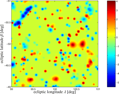
The sensitivity of Planck is good enough to perform an SZ survey of a significant part of the Hubble volume. Because the simulation of such a vast volume including hydrodynamics resolving scales as small as cluster substructure is beyond the capabilities of current computers, a hybrid approach has been pursued for the map construction. All-sky maps of the SZ sky were constructed by using the light-cone output of the Hubble-volume simulation (Colberg et al. 2000; Jenkins et al. 2001) as a cluster catalogue and template clusters from the small-scale gas-dynamical simulation (White et al. 2002). In this way, sky maps were constructed which contain all clusters above 5 × 10¹³ M_⊙/h out to redshift z= 1.48. The maps show the right two-point halo correlation function, incorporate the evolution of the mass function and the correct distribution of angular sizes. Furthermore, they exhibit cluster substructure and deviations from the ideal cluster scaling relations induced, for example, by the departure from spherical symmetry. The velocities used for computing the kinetic SZ effect correspond to the ambient density field. The map construction process and the properties of the resulting map are in detail described in Schäfer et al. (2006a). Details of the thermal and kinetic SZ maps can be seen in Figs 1 and 2, respectively.

Figure 1

Open in new tabDownload slide

Detail of the thermal Comptonization map: a 2 × 2-deg² wide cut-out centred on the ecliptic coordinates (λ, β) = (100°, − 50°) is shown. The smoothing imposed was a Gaussian kernel with Δθ= 2.0 arcmin [full width at half-maximum (FWHM)]. The shading indicates the value of the thermal Comptonization y, which is proportional to arsinh (10⁶y). The mesh size of the underlying Cartesian grid is ∼14 arcsec.

Figure 2

Open in new tabDownload slide

Detail of the kinetic Comptonization map: a 2 × 2-deg² wide cut-out is shown centred on the same position as Fig. 1, that is, at the ecliptic coordinates (λ, β) = (100°, −50°). The smoothing imposed was a Gaussian kernel with Δθ= 2.0 arcmin (FWHM). The kinetic Comptonization w is indicated by the shading, being proportional to arsinh (10⁶w).

3 SIMULATION OF SZ OBSERVATIONS WITH Planck

In this section, the simulation is outlined. First, the foreground emission components considered are summarized (Sections 3.1 and 3.2), and instrumental issues connected to submillimetric observations with Planck are discussed (Section 3.3). The data products resulting from the simulation at this point will be spherical harmonics expansion coefficients 〈S_ℓm〉_ν of the flux maps S_ν(θ) for all nine observing frequencies ν, where the spectra have been convolved with Planck's frequency response windows and the spatial resolution of each channel is properly accounted for. Next, the signal extraction methodology based on matched and scale-adaptive filtering is described (Section 3.4), followed by considering a toy model for the efficiency of the filter algorithm under additional noise contributions (3.5) and the application to simulated Planck data (Section 3.6). The morphology of peaks in the filtered maps as a function of signal profile model parameters is discussed (Section 3.7) and finally the algorithm for the extraction of peaks in the filtered maps and the identification with objects in the cluster catalogue is described (Section 3.8). A description of the software tools and the foreground modelling used for our simulation can be found in Reinecke et al. (2006).

3.1 Foreground components

We assume that the spectral properties of each emission component are isotropic, and that the amplitude of the emission is described by a suitably extrapolated template. It should be emphasized that this assumption is likely to be challenged, but the lack of observations makes it difficult to employ a more realistic scheme. Furthermore, it should be kept in mind that the extrapolation of the Galactic emission components by as much as three orders of magnitude in the case of synchrotron radiation is insecure. Details of the templates and the various emission laws are given in a precursor paper (Schäfer et al. 2006b).

• CMB: From the spectrum of C_ℓ-coefficients generated with cmbfast (Seljak & Zaldarriaga 1996) for the assumed ΛCDM cosmology, a set of a_ℓm-coefficients was derived by using the synalm code based on synfast by Hivon et al. (1998).

• Galactic synchrotron emission: The modelling of the Galactic synchrotron emission was based on an observation carried out by Haslam et al. (1981, 1982) at an observing frequency of ν= 408 MHz, which has been adopted for Planck usage by Giardino et al. (2002). The spectral law for extrapolating the synchrotron flux incorporates a spectral break at ν= 22 GHz, which has been reported by the Wilkinson Microwave Anisotropy Probe (WMAP) satellite.

• Galactic dust emission: The thermal emission from Galactic dust (Schlegel et al. 1998) used a two temperature model proposed by C. Baccigalupi, which yields a good approximation to the model introduced by D. J. Schlegel. The emission is modelled by a superposition of two Planck laws with temperatures T₁= 9.4 K and T₂= 16.2 K at a fixed ratio.

• Galactic free–free emission: Modelling of the Galactic free–free emission was based on an H_α-template provided by Finkbeiner (2003) and the spectral model proposed by Valls-Gabaud (1998), which employs an approximate conversion from the H_α intensity to the free–free intensity parametrized with the plasma temperature and describes the spectral dependence of the free–free brightness temperature with a ν⁻²-law.

• Emission from carbon monoxide in giant molecular clouds: Rotational transitions of carbon monoxide give rise to a series of lines at integer multiples of the frequency ν_CO= 115 GHz. Its strength is given by the template provided by Dame et al. (1996, 2001). The line strengths of higher harmonics of the transition were determined by assuming thermal equilibrium of the molecular rotational states with an ambient temperature of T_CO= 20 K.

• Emission from planetary bodies of the Solar System: We considered a model of the heat budget of the planetary surface with periodic heat loading from the Sun and internal sources of thermal energy, heat emission and conduction to the planet's atmosphere and the back-scattering on to the surface by the atmosphere. From the orbital elements of the planet as well as from the motion of the Lagrange point L₂ where Planck will be positioned we derived the distance to the planet and its position in order to compute a sky map. In total, we considered 1200 asteroids apart from the five (outer) planets, excluding Pluto which is too faint to be detected by Planck.

3.2 Omitted foreground components

The list of foreground emission components which possibly hamper the observation of SZ clusters is still not complete. Microwave point sources such as active galactic nuclei (AGNs) and star-forming galaxies were not included, likewise the modelling of zodiacal light originating from interplanetary dust in the Solar System was not attempted. Concise descriptions of Galactic foregrounds at CMB frequencies derived from WMAP data are given by (Bennett et al. 2003) and Patanchon et al. (2005).

The reason why we did not attempt to model noise originating from AGNs and infrared star-forming galaxies, despite unequivocally constituting an important noise source for Planck, is the great uncertainty of their spectral behaviour and clustering properties, their biasing, and in the case of AGNs, their duty cycles. For a detailed discussion we refer the reader to Schäfer et al. (2006b), and in Section 3.5, we provide a discussion of a toy model explaining how the filter efficiency is affected by the inclusion of additional noise sources.

3.3 Instrumental issues

The most important aspects related to the observations of the CMB sky by Planck are the properties of the optical system, the noise introduced by the receivers and the frequency response, which will be summarized in this section:

• Planck beam shapes: The beam shapes of Planck are approximated by azimuthally symmetric Gaussians with ⁠. The residuals from the idealized Gaussian shape are expected not to exceed the per cent level. Table 1 gives the angular resolution Δθ for each channel.

• Simulation of noise maps: Noise maps were generated by drawing Gaussian distributed random numbers from a distribution with zero mean and variance σ_N given by Table 1. These numbers correspond to the noise for a single observation of a pixel by a single detector. Consequently, this number is down-weighted by (assuming Poissonian statistics), where n_det denotes the number of redundant receivers per channel, because they provide independent surveys of the microwave sky. In a second step, exposure maps were derived by simulating scan paths with Planck mission characteristics. Using the number of observations n_obs per pixel, it is possible to scale down the noise amplitudes by and to obtain a realistic noise map for each channel.

• Frequency response and superposition of emission components: Adopting the approximation of isotropy of the emission component's spectral behaviour, the steps in constructing spherical harmonics expansion coefficients of the flux maps S(θ, ν) for all Planck channels consist of deriving the expansion coefficients a_ℓm of the template a(θ),

  

  8
  converting the template amplitudes a_ℓm to fluxes S_ℓm, extrapolate the fluxes with a known or assumed spectral emission law to Planck's observing frequencies, to finally convolve the spectrum with Planck's frequency response window for computing the spherical harmonics expansion coefficients of the average measured flux at nominal frequency ν₀ by using:

  

  9
  Here, S_ℓm(ν) describes the spectral dependence of the emission component considered, and the frequency response of Planck's receivers centred on the fiducial frequency ν₀. For all its channels, Planck's frequency response function is well approximated by a top-hat function:

  

  10

  The centre frequencies ν₀ and frequency windows Δν for Planck's receivers are summarized in Table 1. In the final step, the averaged fluxes for each emission component are added to yield the expansion coefficients of the flux map.

3.4 Construction of optimized filter kernels

The basis of our signal extraction method is the concept of matched and scale-adaptive filtering pioneered by Sanz et al. (2001) and Herranz et al. (2002), which we generalized to the case of spherical data sets and spherical harmonics Y_ℓm(θ) as the harmonic system replacing Fourier transforms and plane waves of the case of a flat geometry. The theory of matched and scale-adaptive filtering of multifrequency data sets is beautifully developed by the above mentioned authors in their formulation as the solution to a functional variation problem with increasing complexity. Filter kernels ψ(|θ|, R) constructed for finding objects of a certain scale R modify the sky map w(θ) by convolution and are required to minimize the variance σ²_w(R) of the filtered map w(θ, R) while fulfilling certain conditions:

• there should exist a scale R₀ for which the value of the filtered field 〈w(R₀)〉 at the position of a source is maximal,

• the filter should be unbiased, that is, 〈w(R₀)〉 at the position of a source should be proportional to the amplitude of the underlying signal and

• the variance σ²_w(R) should have a minimum at this scale R₀.

In short, the filtered field should yield maximized signal-to-noise ratio values for the peaks, while being linear in the signal and allowing the measurement of sizes of objects. We restrict ourselves to spherically symmetric source profiles superimposed on a fluctuating background which is a realization of a homogeneous and isotropic Gaussian random field characterized by its power spectrum. The filter resulting from the variation with the boundary conditions (i) and (ii) is called matched filter, and the filter obeying all three conditions is referred to as the scale-adaptive filter.

Solving this variational problem in its extension to multifrequency data and spherical maps yields spherical harmonics expansion coefficients ψ_ν(ℓ) for the filter kernels of each observational channel ν as a function of the assumed profile of the source, of the spectral variation of the source flux with frequency and of the auto- and cross-correlation power spectra ⁠. The relative normalization of the filter kernels in different channels encodes the optimized linear combination coefficients for co-adding the filtered maps. Apart from that, one obtains an analytical expression for the fluctuation amplitude of the filtered and co-added maps, such that any peak height can be expressed in units of the map's s.d., which directly allows to quantify whether a certain peak is likely to be a genuine signal or a mere background fluctuation.

Filter kernels following from the matched and scale-adaptive multifrequency filtering algorithm were subjected to a thorough analysis. They are tested on two different data sets, one containing just CMB fluctuations and (non-isotropic) instrumental noise, and a second data set, which comprises all foregrounds in addition. From the comparison of the two data sets one will be able to quantify by how much the number of detections drop due to the foreground components and how uniform the cluster distribution will be provided the removal of foregrounds can be done efficiently. Details of the cross-channel correlation properties of the foregrounds as well as of the noise and the derivation of filter kernels and their properties are discussed in a pre-cursing paper (Schäfer et al. 2006b).

It is worthwhile mentioning that the method can be equally well applied to the case, where the foreground emission components show position dependent spectral properties. In this case, however, one would need to derive the cross-power spectra from the expansion coefficients a_ℓm, which follow from a simulated sky map adding all emission components with the correct position dependent spectral weighting. The assumption of a constant spectral behaviour of a template allows a significant simplification of the simulation by adding expansion coefficients a_ℓm with an overall spectral dependence and to determine the cross-power spectra from those.

3.5 Influence of a point source population on the filter efficiencies

In order to quantify the effect of an additional noise contribution on the detectability of the SZ clusters and on the efficiency of the filtering algorithms, we consider a simplified toy model, discussed in more detail in Schäfer et al. (2006b). Specifically, a circularly symmetric source profile τ(θ) of Gaussian shape,

11

is superimposed on a fluctuating background, with the angular power spectrum C(ℓ) describing the fluctuation statistics. For illustrative purposes, the derivation is restricted to matched filtering of a single-frequency observation, and the computation is carried out on a plane tangential to the celestial sphere, where the small-angle approximation is valid.

The power spectrum of the noise now combines uncorrelated pixel noise, for which C(ℓ) ∝ℓ² with the contribution due to uncorrelated point sources, modelled by C(ℓ) ∝ℓ^α. The variable q adjusts the relative normalization of the noise models and the exponent α is left as a free parameter in order to include deviations from a pure Poissonian process:

12

Using the formulae in Schäfer et al. (2006b), the Fourier-transformed matched filter ψ(ℓ) is given by

13

The signal-to-noise ratios of a peak are given by

14

before filtering and by

15

after filtering. The gain ratio Q, quantifying the increase in the signal-to-noise ratio due to filtering relative to an unfiltered data set, is defined as

16

Fig. 3 summarizes the results. The gain ratio Q is depicted as a function of the relative normalization q, from q= 0.1 (negligible point source contribution) to q= 10 (dominating point source contribution) and of the power-law slope α. Q(q, α) is normalized to the value of Q for q= 0.1 and α= 1, that is, for a negligible contribution of the point sources to the noise power spectrum. Thus, the plot characterizes the decrease in gain Q in the signal-to-noise ratio if the noise power spectrum C(ℓ) contains an additional point source contribution relative to the case where C(ℓ) reflects only instrumental noise.

Figure 3

Open in new tabDownload slide

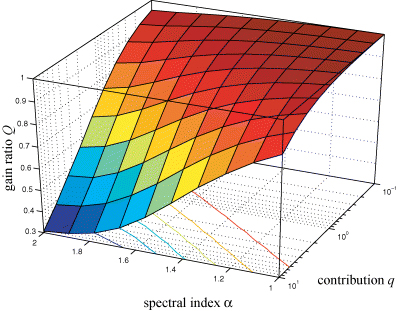
Gain factor Q≡D_u/D_s for a noise model combining instrumental noise and point sources, as a function of power-law index α and amplitude q of the point source angular power spectrum.

For a realistic value of α= 2 one observes a decrease in Q by 30 per cent in the case q= 1, that is, if the power spectra of the instrumental noise and that of the point sources are of equal magnitude, which seems to be substantial modification of the noise power spectrum. This trend getting weaker for flatter power-law indices α and is proportional to log (q) to a good approximation. In the above considerations, the core size θ_c was kept fixed at 10 arcmin.

3.6 Filter construction and synthesis of likelihood maps

Filter kernels optimized for detecting a family of King-profiles y(θ) ∝[1 + (θ/θ_c)²]^−λ were derived for a range of core radii θ_c and asymptotic slopes λ. Specifically, seven values of θ_c,

17

and five values of λ,

18

were considered, keeping the large range in core radii in mind. Using different values for λ is motivated by deviations from the generic baryonic profile and by asymmetric clusters. The sky maps were convolved with the filter kernels, co-added, normalized to unit variance, as described in the previous section and synthesized to yield likelihood maps. In the synthesis, all multipole coefficients up to ℓ= 4096 have been considered and the angular resolution of the resulting maps (N_side= 1024, pixel side length ≃3.4 arcmin) is high enough to resolve single likelihood peaks.

An important numerical issue of spherical harmonic transforms is the fact that the variance (measured in real space) of a map synthesized from the a_ℓm-coefficients is systematically smaller with increasing ℓ than the variance C(ℓ) required by the a_ℓm-coefficients on the scale Δθ≃π/ℓ. This is compensated by an empirical function, the so-called pixel window, which lifts the amplitudes a_ℓm towards increasing values of ℓ prior to the reconstruction (Hivon et al. 1998). This effectively results in higher signal-to-noise ratios of the detected clusters. In the numerical derivation of filter kernels very low multipoles below ℓ≤ 3 were excluded because of numerical instabilities in a matrix inversion and set artificially to zero. An important consequence of this will be discussed in Section 4.7.

3.7 Morphology of SZ clusters in filtered sky maps

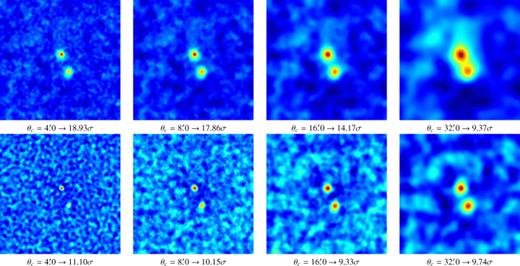
Fig. 4 gives an impression how the morphology of a peak in the likelihood map changes if filter kernels optimized for the detection of profiles with varying diameter and asymptotic behaviour are used. We picked an association of two clusters at a redshift of z≃ 0.1, which generates a signal strong enough to yield a significant detection irrespective of the choice of θ_c and λ.

Figure 4

Open in new tabDownload slide

An association of two clusters at z≃ 0.1, extracted with the matched multifilter (top row) and with the scale-adaptive multifilter (bottom row) from a map containing all Galactic components, CMB fluctuations and instrumental noise. The panel gives the likelihood maps and the statistical significances of the detection of the cluster at the image centre in units of σ, for varying values of θ_c with λ fixed at λ= 1.0. The side length of the panels is 4°.

The matched filter yields larger values for the detection significance, which is defined to be the signal-to-noise ratio of the central object, in comparison to the scale-adaptive filter for that particular pair of clusters. Secondly, if filters optimized for large objects, that is, large θ_c and small λ are used, the two peaks merge in the case of the matched filter, but stay separated in case of the scale-adaptive filter. Hence the scale-adaptive filter is more appropriate in the investigation of neighbouring objects. Additionally, the matched filter seems to be more sensitive to the choice of θ_c and λ. Within the range of these two parameters considered here, the significance of the cluster detection under consideration varies by a factor of 4 in the case of the matched filter, but changes only by 25 per cent in the case of the scale-adaptive filter.

3.8 Peak extraction and cluster identification

It is an important point to notice that cluster positions derived from Planck are not very accurate. In this analysis, the SZ clusters are extended themselves and possibly asymmetric, they are convolved with Planck's instrumental beams in the observation and reconstructed from filtered data, where an additional convolution with a kernel is carried out. Furthermore, the pixelization is relatively coarse (typically a few arcmin). All these effects add up to a position uncertainty of a few tens of arcminutes, depending on the filter kernel.

All peaks above 3σ were extracted from the synthesized likelihood maps and cross-checked with a cluster catalogue. A peak was taken to be a detection of a cluster if its position did not deviate more than 30.0 arcmin from the nominal cluster position. Peaks that did not have a counterpart with integrated Comptonization larger than a predefined threshold value were registered as false detections, likewise peaks were not considered that did not exceed the threshold value of 3σ in more than two contiguous pixels. In this way, a catalogue is obtained which is essentially free of false detections and where the fraction of unidentified peaks amounts to 5–7 per cent for a realistic threshold of (Haehnelt 1997; Bartelmann 2001). The cluster catalogues following from observations with specific (θ_c, λ)-pairs of parameters were merged to yield summary catalogues for both filter algorithms and both noise compositions. If more than one cluster is found in the aperture, the cluster with the largest value for the integrated Comptonization is assumed to generate the signal. In the merging process, we determine which choice of (θ_c, λ) yielded the most significant detection for a given object.

4 RESULTS

First of all, we investigate the noise properties of the likelihood maps (Section 4.1), followed by an analysis of the detection significances (Section 4.2) the different filter algorithms are able to yield. Then, the number of detected clusters as a function of model profile parameters is investigated (Section 4.3). The population of SZ clusters in the mass–redshift plane (Section 4.4), the distribution of the position accuracies (Section 4.6) and the spatial distribution of clusters (Section 4.7) are the main results of this work. Finally, the detectability of the kinematic SZ effect is addressed (Section 4.5).

4.1 Noise in the filtered and co-added maps

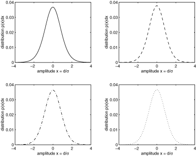
In this section, the statistical properties of the noise in the filtered maps are examined. The filter construction algorithm gives the variance σ of the filtered and co-added fields as a function of filter shapes and cross-channel power spectra by virtue of ⁠. Due to deviations from Gaussianity of many noise components considered (especially Galactic foregrounds), it is important to verify if the variance is still a sensible number. Fig. 5 gives the distribution of pixel amplitudes for a combination of noise components and filtering schemes.

Figure 5

Open in new tabDownload slide

Distribution of pixel amplitudes d of the filtered and co-added maps, normalized to the variance σ predicted in the filter kernel derivation, for a data set including CMB fluctuations and instrumental noise, filtered with the matched filter (upper left-hand panel, solid line), for a data set including Galactic foregrounds in addition (upper right-hand panel, dashed line), for a data set containing the CMB and instrumental noise, filtered with the scale-adaptive filter (lower left-hand panel, dash–dotted line) and finally a data set with CMB, instrumental noise and Galactic foregrounds, filtered with the scale-adaptive filter (lower right-hand panel, dotted line). The filters have been optimized for the detection of beam-shaped profiles.

Although the distribution of pixel amplitudes seems to follow a Gaussian distribution with zero mean and unit variance in all cases, there are slight deviations from this first impression. As summarized in Table 2, the mean of the distributions is compatible with zero in all cases, but the s.d. is less than unity. Furthermore, the kurtosis of all distributions is non-zero, hence they are more outlier-prone as the normal distribution (barykurtic), which leads to a misestimation of statistical significances of peaks based on the assumption of unit variance of the filtered map, which the filtered map should have due to the renormalization. This effect is strongest in the case of the matched filter. For the derivation of these numbers, only pixels with amplitudes smaller than |d| ≤ 4σ have been considered, such that the statistical quantities are dominated by the noise to be examined and not by the actual signal. The distributions are slightly skewed towards positive values, which is caused by weak signals below 4σ. The near-Gaussianity suggests that the residual noise in the filtered map is mostly caused by uncorrelated pixel noise and filters seem to be well capable of suppressing unwanted foregrounds.

Is it important to notice that the comparatively low threshold of 3σ imposed for extracting the peaks alone would yield a considerable number of false detections. This motivated the rather complicated algorithm outlined in Section 3.8. Supposing that the variance of the filtered maps is mainly caused by uncorrelated pixel noise which is smoothed to an angular scale of ≃20 arcmin by the instrumental beam and by the filters causes the filtered maps to be composed of 4π(180/π)²× 3²≃ 4 × 10⁵ unconnected patches. Of these patches, a fraction of naturally fluctuates above the threshold of 3σ. In this way a total number of ≃400 patches have significances above 3σ. The requirement that the counterpart of the peak in the cluster catalogue generates a Comptonization above a (conservative) value of ⁠, that is, that a cluster candidate is confirmed by spectroscopy, removes these false peaks from the data sample.

4.2 Detection significances and total number of detections

The distribution of detection significances is given in Fig. 6. One obtains about 10³ detections at the significance threshold which drops to a few highly significant detections exceeding 20σ. At small σ, the scale-adaptive filter yields more detections than the matched filter, which catches up at roughly 5σ.

Figure 6

Open in new tabDownload slide

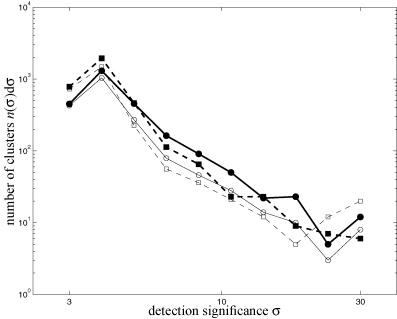
Distribution n(σ)dσ of the detection significances σ, for the matched filter (solid line, circles) in comparison to the scale-adaptive filter (dashed line, squares). The distributions are given for the clean data set including only the CMB, both SZ effects and instrumental noise (thick lines, closed symbols) and in comparison, the data set where all Galactic foreground components are included in addition (thin lines, open symbols).

The total number of detections for each filter algorithm, for each data set and for two values of the minimally required Comptonization for spectroscopic confirmation are compiled in Table 3. Due to its better yield of detections marginally above the threshold the scale-adaptive filter outperforms the matched filter by almost 30 per cent. The reason for the increased number of low-significance detections is the systematically higher value of the variance of the residual noise field in the case of the scale-adaptive filter. The number of detections decreases by ≃25 per cent if Galactic foregrounds are included, relative to the data set containing only CMB fluctuations and instrumental noise. In a realistic observation, one can expect a total number of ∼6 × 10³ clusters of galaxies, compared to ≃8 × 10³ clusters if only the CMB and instrumental noise were present. When comparing the total number of detections to analytic estimates (e.g. Aghanim et al. 1997; Bartelmann 2001; Kay et al. 2001), it is found that the number of clusters detected here is smaller, by a factor of <2.

Table 3

Total number of detections in both data sets and with both filters, and for two values for minimally required Comptonization.

Filter algorithm	Data set
Matched filter	CMB + noise	2402	5376
Matched filter	CMB + noise + Galaxy	1801	4199
Scale-adaptive filter	CMB + noise	3234	8020
Scale-adaptive filter	CMB + noise + Galaxy	2428	6270

Filter algorithm	Data set
Matched filter	CMB + noise	2402	5376
Matched filter	CMB + noise + Galaxy	1801	4199
Scale-adaptive filter	CMB + noise	3234	8020
Scale-adaptive filter	CMB + noise + Galaxy	2428	6270

Open in new tab

Table 3

Total number of detections in both data sets and with both filters, and for two values for minimally required Comptonization.

Filter algorithm	Data set
Matched filter	CMB + noise	2402	5376
Matched filter	CMB + noise + Galaxy	1801	4199
Scale-adaptive filter	CMB + noise	3234	8020
Scale-adaptive filter	CMB + noise + Galaxy	2428	6270

Filter algorithm	Data set
Matched filter	CMB + noise	2402	5376
Matched filter	CMB + noise + Galaxy	1801	4199
Scale-adaptive filter	CMB + noise	3234	8020
Scale-adaptive filter	CMB + noise + Galaxy	2428	6270

Open in new tab

One should keep in mind that the noise due to Planck's scanning paths is highly structured on the cluster scale and below. This has two important consequences. First, assuming a simple flux detection threshold in analytic estimates is not valid and secondly the assumption of isotropy which is essential to the filter construction is violated which affects the sensitivity of the filters, and decreases the number of detections.

The low value of σ₈≃ 0.75 measured by WMAP has a dramatic influence on the cluster number counts. At the high masses considered here, the number of objects is reduced by a factor of roughly 3, making the number of highly significant detections comparable to already existing cluster catalogues, for example, the REFLEX sample from the ROSAT all-sky survey (Böhringer et al. 2004). On the other hand, the value σ₈= 0.9 used in this work is still supported by weak cosmic shear measurements and is in fact favoured by common likelihood contours of CMB and weak lensing data (Spergel et al. 2006).

4.3 Cluster detectability as a function of filter parameters

The way the significance of a detection of a cluster changes when the core size θ_c and the asymptotic slope λ are varied is illustrated in Fig. 4 for the matched filter. In general, the matched filter yields significances that are almost twice as large in comparison to the scale-adaptive filter for the specific example considered and consequently finds more clusters above a certain detection threshold. Furthermore, the matched filter shows a stronger dependence of the significance on the filter parameters θ_c and λ. The significance for the detection of the same object varies by a factor of 4 in case of the matched filter but only by 25 per cent in the case of the scale-adaptive filter. This means that the derivation of cluster properties based on the filter parameter that yielded the most significant detection is likely to work for the matched filter, but not for the scale-adaptive filter. It should be emphasized, however, that the scale-adaptive filter keeps the likelihood distributions of the two objects from merging, in contrast to the matched filter. For that reason, the scale-adaptive filter may be better suited for the investigation of associations and pairs of SZ clusters.

Fig. 7 shows the number density of detectable clusters as a function of the King-profile's core size θ_c that entered the filter construction. Whereas the matched filter yields most detections at small values of θ_c, the scale-adaptive filter is better suited to detect extended objects. Most of the detections are registered at core sizes θ_c= 8 arcmin. Additionally, the scale-adaptive filter's capability of detecting extended objects suffers from the inclusion of Galactic foregrounds, which cause the total number of detections to drop by 20 per cent. In contrast, the matched filter is able to deliver a comparable performance for all values of θ_c if Galactic foregrounds are included.

Figure 7

Open in new tabDownload slide

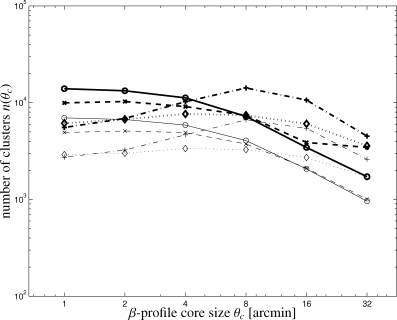
Number density n(θ_c) of clusters as a function of the filter parameter core size θ_c, for a data set including CMB fluctuations and instrumental noise, filtered with the matched filter (circles, solid line), for a data set including Galactic foregrounds in addition (crosses, dashed line), for a data set containing the CMB and instrumental noise, filtered with the scale-adaptive filter (plus signs, dash–dotted line) and finally a data set with CMB, instrumental noise and Galactic foregrounds, filtered with the scale-adaptive filter (diamonds, dotted line). The thick and thin lines denote detections and peaks above 10⁻³ and 3 × 10⁻⁴ arcmin², respectively.

The number density of clusters as a function of the King-profile's asymptotic slope λ which the filters are optimized for is given in Fig. 8. The number of detections following from scale-adaptive filtering is relatively insensitive to particular choices of λ, whereas the matched filter yields a higher number of detections in the case of compact objects, irrespective of the noise components included in the analysis. Fig. 9 illustrates how the number of detections changes as a function of both θ_c and λ. It should be emphasized that none of the graphs depicted in Figs 7–9 shows the total number of detections for a given choice of θ_c and λ and that graphs are not corrected for multiple detections of objects at more than (θ_c, λ)-pair.

Figure 8

Open in new tabDownload slide

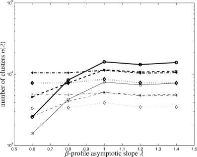
Number density n(λ) of clusters as a function of the filter parameter asymptotic slope λ, for a data set including CMB fluctuations and instrumental noise, filtered with the matched filter (circles, solid line), for a data set including Galactic foregrounds in addition (crosses, dashed line), for a data set containing the CMB and instrumental noise, filtered with the scale-adaptive filter (plus signs, dash–dotted line) and finally a data set with CMB, instrumental noise and Galactic foregrounds, filtered with the scale-adaptive filter (diamonds, dotted line). The thick and thin lines denote detections and peaks above 10⁻³ arcmin² and 3 × 10⁻⁴ arcmin², respectively.

Figure 9

Open in new tabDownload slide

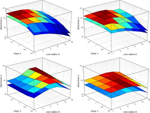
Number of detections n(θ_c, λ) as a function of both filter parameters core size θ_c and asymptotic slope λ, for the matched filter (top row) in comparison to the scale-adaptive filter (bottom row). The figure compares the number density following from a clean data set containing the CMB, the SZ effects and instrumental noise (left-hand column) with a data set containing all Galactic components in addition (right-hand column). n(θ_c, λ) is given for the minimal signal strength (upper plane) compared to (lower plane).

4.4 Cluster population in the M–z plane

Scatter plots describing the population of detectable clusters in the mass–redshift plane are shown in Fig 10 for the matched filter and in Fig. 11 for the scale-adaptive filter. The clusters populate the log(M)–z plane in a fairly well defined region. There are only few detections beyond redshifts of z= 0.8, but the shape of the detection criterion suggests the existence of a region of low-mass low-redshift clusters which should be detectable but which are not included in the map construction. It is difficult to predict the SZ properties of low-mass clusters because many complications in the sector of baryonic physics come into play such as preheating, deviation from scaling laws and incomplete ionization, which makes it difficult to predict the number of clusters missing in our analysis. Together with K. Dolag we prepared an auxiliary SZ map from a gas-dynamical constrained simulation of the local universe that would fill in the gap and provide clusters with masses M < 5 × 10¹³ M_⊙/h below redshifts of z < 0.1 (Dolag et al. 2005).

Figure 10

Open in new tabDownload slide

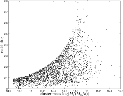
Population of clusters in the log (M) –z plane detected with the matched multifilter for the data set containing the CMB, instrumental noise and all Galactic foregrounds. The minimal signal strength was required to be ⁠.

Figure 11

Open in new tabDownload slide

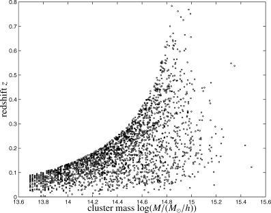
Population of clusters in the log(M)–z plane detected with the scale-adaptive multifilter. Here, the detections are given for a data set containing the CMB, instrumental noise and all Galactic foregrounds. All peaks exceed a minimal Comptonization of ⁠.

Fig. 12 gives the marginalized distribution in redshift z of the cluster sample. The shape of the redshift distribution is determined by the competition of two effects. With increasing redshift z the observed volume increases, but contrariwise, the number of massive clusters decreases as described by the Press–Schechter function and the SZ signal becomes smaller proportional to d⁻²_A (z). Most of the clusters are observed at redshifts of z≃ 0.2 and the detection limit is reached at redshifts of z≃ 0.8. This applies to both filter algorithms and data sets alike.

Figure 12

Open in new tabDownload slide

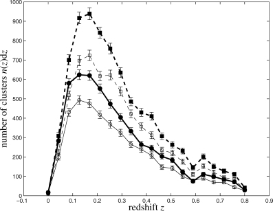
Distribution n(z) dz of the detected clusters in redshift z, for the matched filter (solid line, circles) in comparison to the scale-adaptive filter (dashed line, squares). The figure compares detections in a clean data set containing the CMB, both SZ effects and instrumental noise (thick lines, closed symbols) to a data set with all Galactic components in addition (thin lines, open symbols). Again was set to 3 × 10⁻⁴ arcmin².

Fig. 13 gives the marginalized distribution of the cluster's logarithmic mass m= log [M/(M_⊙/h)]. At high masses, both filtering schemes detect cluster reliably, but with decreasing mass, the filter algorithms start to show differences in their efficiency. The mass functions peak at a value of 2.5 × 10¹⁴ M_⊙/h, and decrease towards smaller values for the mass due to the decrease in SZ signal strength ⁠. Fig. 14 gives the distribution of the cluster's Compton- parameter. The distribution is close to a power law as expected from virial estimates (cf. Schäfer et al. 2006a), but at low Comptonizations, all distributions evolve more shallowly, which is due to the fact that clusters fail to generate a peak in the likelihood map exceeding the threshold value.

Figure 13

Open in new tabDownload slide

Distribution n(m) d m of the detected clusters in logarithmic mass m= log [M/(M_⊙/h)], for the matched filter (solid line, circles) in comparison to the scale-adaptive filter (dashed line, squares). Here, the distributions are given for a data set including only the CMB, both SZ effects and instrumental noise (thick lines, closed symbols) in comparison to a data set containing moreover all Galactic foreground emission components (thin lines, open symbols). The minimal Comptonization for spectroscopic confirmation was ⁠.

Figure 14

Open in new tabDownload slide

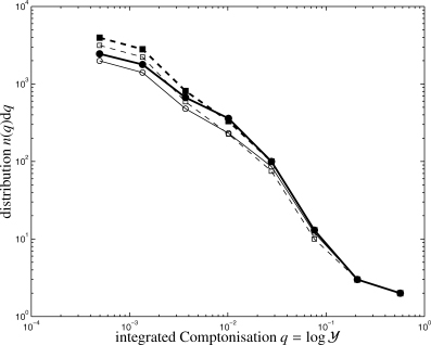
Distribution n(q)dq of the logarithmic integrated Comptonization, ⁠, for the matched filter (solid line, circles) in comparison to the scale-adaptive filter (dashed line, squares). Here, the distributions are given for a data set including only the CMB, both SZ effects and instrumental noise (thick lines, closed symbols) in comparison to a data set containing moreover all Galactic foreground emission components (thin lines, open symbols).

4.5 Linearity of the multifilters

Figs 15 and 16 show the linear response of the amplitude of the filtered co-added field to the underlying signal. They show a correlation between the integrated Comptonization of the SZ cluster and the amplitude of the filtered field, expressed in units of the rms fluctuations of the filtered field. The correlation increases with increasing significance, and the scatter decreases from one order of magnitude close to the detection threshold to 0.2 dex at high detection significances.

Figure 15

Open in new tabDownload slide

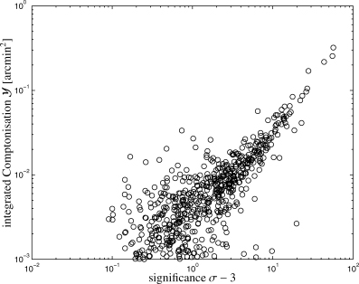
Dependence between the statistical significance and the Comptonization of the detections, for the matched multifilter, which has been optimized for finding objects with θ_c= 4.0 arcmin and asymptotic slope λ= 1.0, for the complete data set.

Figure 16

Open in new tabDownload slide

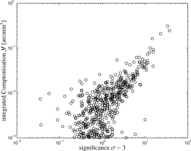
Dependence between the statistical significance and the Comptonization of the detections, for the scale-adaptive multifilter, which has been optimized for finding objects with θ_c= 8.0 arcmin and asymptotic slope λ= 1.0, for the complete data set.

Quite generally, the statistical significance of a detection and the Comptonization of the underlying cluster are related by a power law with a slope close to unity, which enables the direct estimation of the cluster parameters. The data are plotted for Comptonizations exceeding 10⁻³ arcmin², below which no clear trend with significance of the peak can be seen, and for a specific value of the filter parameters θ_c and λ, because the relations differ in normalization for varying choices of θ_c and λ. Thus, the requirement of linearity of the amplitude of the filtered field with the signal of the object to be detected, which was one of the axioms of filter construction, is verified.

4.6 Position accuracies

A histogram of the deviations between actual and reconstructed cluster position is given by Fig. 17. The position accuracy is given in terms of the squared angular distance Δ=θ²_arc because a uniform distribution would yield a flat histogram, as the bins are comprise equal solid angle elements. The distribution is sharply peaked towards Δ= 0 arcmin². A fraction of 50 per cent of all clusters are detected within 10 arcmin from the nominal source position, but there is a tail in the distribution towards larger angular separations. For most of the clusters, this position accuracy is good enough for direct follow-up studies at X-ray wavelengths, but not good enough for optical observations.

Figure 17

Open in new tabDownload slide

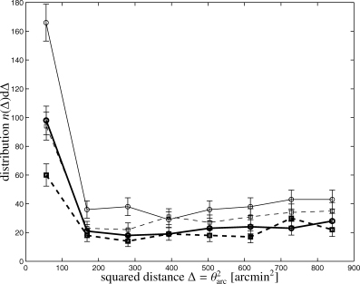
Distribution of the squared angular distance Δ=θ²_arc between actual and reconstructed source position on a great circle, for the matched filter (solid line, circles) in comparison to the scale-adaptive filter (dashed line, squares). The figure compares detections above 4σ (thin lines) with detections above 5σ for clusters detected with the parameter θ_c= 8.0 arcmin. The clusters were required to generate a Comptonization exceeding 3 × 10⁻⁴ arcmin².

As noticed in Herranz et al. (2002), it is not trivial to assign a peak in the filtered co-added map to an actual underlying cluster. The size of the error circle was chosen by the following consideration on the error budget. The Planck beams have a sensitivity-averaged extension of ≃10 arcmin, the filter kernels provide an additional smoothing depending on the choice of θ_c and λ with ≃20 arcmin being a typical value, and the pixelization of the likelihood-map synthesized from the filtered spherical harmonics expansion coefficients amounts to ≃4 arcmin. Cluster substructure and systematic displacements of the peak of the SZ decrement relative to the clusters barycentre and displacements of the barycentre relative to the most bound particle of the simulation are smaller than 1 arcmin and are therefore neglected.

Adding these values in quadrature yields a value of 24 arcmin, which was extended to 30 arcmin. When considering an error circle of that size, there is a significant chance of a random erroneous match between a fluctuation and a cluster in the source catalogue. With 10⁴ clusters generating a Comptonization exceeding 3 × 10⁻⁴ arcmin², the probability for random match is smaller than 20 per cent, which was considered to be an acceptable contamination. It should be kept in mind, that for Gaussian statistics, which is strongly supported by the results of Section 4.1, one expects only of the order of 400 random fluctuations above 3σ without any counterpart, which would ultimately generate ≃80 false matches with the source catalogue, which is a small number compared to the number of entries in the cluster catalogues.

4.7 Spatial distribution of Planck's SZ cluster sample

Fig. 18 shows the number density of clusters as a function of ecliptic latitude y≡ cos β. The figure states that the Planck cluster sample extracted with the specific filters is highly non-uniform for low significance thresholds, where most of the clusters are detected on a belt around the celestial sphere, but gets increasingly more uniform with higher threshold values for the significance. This is due to the incomplete removal of low-ℓ modes in the filtered maps, which bears interesting analogies to the peak-background split (White et al. 1987; Cole & Kaiser 1989) in biasing schemes for linking galaxy number densities to dark matter densities. Essentially, the likelihood maps are composed of a large number of small-scale fluctuations superimposed on a background exhibiting a large-scale modulation. In regions of increased amplitudes due to the long-wavelength mode one observes an enhanced abundance of peaks above a certain threshold and hence an enhanced abundance of detected objects.

Figure 18

Open in new tabDownload slide

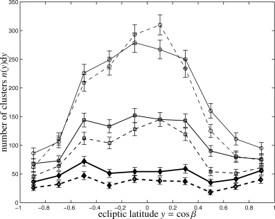
Number n(y)dy of clusters as a function of ecliptic latitude y= cos β, for the matched filter (solid line) in comparison to the scale-adaptive filter (dashed line). The figure compares the number of detected clusters as a function of ecliptic latitude for detection significances >4.2σ (circles, thin lines), >4.8σ (squares, medium lines) and >6.0σ (diamonds, thick lines).

As Fig. 19 indicates, the filtered and co-added maps do have large amplitudes for the hexadecupole which are certainly not in agreement with the near-Poissonian slope of C(ℓ) ∝ℓ² typical for a random distribution of small sources. The incomplete removal of low-ℓ modes shows that the assumptions about isotropy is violated on large scales and C(ℓ) ceases to be a fair description of the variance contained in the a_ℓm-coefficients. Clearly, this is a serious limitation to the spherical harmonic approach. In general, the low-ℓ fluctuations are more pronounced for extended objects, that is, large θ_c and small λ, and they are stronger in the case of the matched filter compared to the scale-adaptive filter.

Figure 19

Open in new tabDownload slide

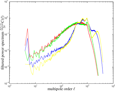
Power spectra C(ℓ) of the filtered and co-added maps, where the filter kernels are derived for the parameters (θ_c, λ) = (4.0 arcmin, 1.0), for the matched filter and data set containing the CMB realization and instrumental noise (red line), for the matched filter and the data set containing all foregrounds in addition (green line), for the scale-adaptive filter and the data set including CMB fluctuations and instrumental noise (blue line) and for the scale-adaptive filter and the data set that contains all foregrounds in addition (yellow line).

Similarly, detection significances near the detection threshold are inaccurate due to the long-wavelength modes. A way to remedy this would be to introduce local estimates of the mean and variance, for example, by considering the average and the s.d. of the amplitudes in an aperture with a few degrees in radius. One must keep in mind that in the filtered map, the signal is strong and likely to affect these two values. It should be emphasized, however, that the strongest signals exceeding values of ≃6σ are uniformly distributed over the celestial sphere.

4.8 Detectability of the kinetic SZ effect

In this section, we give the distribution of peculiar velocities in Planck's SZ cluster sample, which is an important guide for kinetic SZ follow-ups. As Fig. 20 indicates, the distribution of peculiar velocities are well approximated by a Gaussian with zero mean and s.d. σ_vel≃ 300 km s⁻¹. For a dedicated search for the kinetic SZ effect in Planck's SZ cluster sample, velocities are drawn from this distribution, hence cluster bulk motions up to 300 km s⁻¹ can be expected in 68 per cent of all cases and velocities in excess of 1000 km s⁻¹ only for 11–16 objects, depending on the filtering scheme.

Figure 20

Open in new tabDownload slide

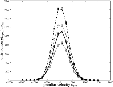
Number n(υ_pec)dυ_pec of clusters, for the matched filter (solid line, circles) in comparison to the scale-adaptive filter (dashed line, squares). Again, the detections in a data set containing the CMB, both SZ effects and instrumental noise (thick lines, closed symbols) are compared to a data set containing all Galactic foregrounds in addition (thin lines, open symbols).

5 SUMMARY AND DISCUSSION

This paper presents the results of a detailed simulation which assesses Planck's capability of detecting SZ clusters. We combine all-sky maps of the SZ effects with templates of Galactic foreground emission components (synchrotron, dust, free–free emission and emission from carbon monoxide molecules), infrared emission from planets and asteroids of the Solar System and noise maps resulting from simulated scan paths, while neglecting the contribution from AGNs due to poorly known spectral properties and biasing properties. The weak SZ signal is amplified and isolated by using matched and scale-adaptive multifrequency filtering.

The properties of the likelihood maps and of the cluster catalogues following from applying matched and scale-adaptive filtering to the simulated flux maps are characterized in detail. According to our simulation, Planck can detect a number of ≃6000 clusters of galaxies in a realistic observation with Galactic foregrounds (compared to over 8000 clusters if only the CMB and instrumental noise were present), which does not confirm the high numbers claimed by analytic estimates.

• The noise properties of the filtered and co-added maps were examined in detail. It was found that the noise is very close to Gaussian after filtering, despite the fact that the initial flux maps had considerable anisotropic non-Gaussian features and despite the fact that the noise is highly structured and anisotropic on the cluster scale. Quantitatively, the variance of the filtered maps is smaller compared to the prediction based on the cross- and auto-correlation functions of the maps convolved with the filter. This discrepancy, which amounts to ≃10 per cent is due to numerics, but has the effect that significances of peaks are slightly underestimated. The cluster detectability as a function of filter parameters showed that the matched filter performs better on compact objects, where its delivered significance depends strongly on the choice of λ. The scale-adaptive filter works well on extended objects and is relatively insensitive to λ.

• The physical properties of the detected SZ cluster sample made in terms of mass M, redshift z and integrated Comptonization ⁠. The cluster population in the mass–redshift plane is fairly well defined, and the marginalization over the mass resulted in most of the clusters being detected at redshifts of z≃ 0.2, where the distribution starts decreasing to values of z≃ 0.8, where no clusters are detected. The distribution of detected SZ clusters in mass M confirmed that the high-mass end of the Press–Schechter function is well sampled, that most of the clusters detected have masses ≃2.5 × 10¹⁴ M_⊙/h and that clusters of lower mass are increasingly difficult to detect.

• The position accuracy is better than 10 arcmin in half of the cases, which is sufficient for X-ray follow-up studies, but the distribution exhibits a tail towards high discrepancies between the cluster position and the position of the peak in the likelihood map.

• The investigation of the spatial distribution, especially in ecliptic latitude showed that the distribution of clusters gets increasingly uniform with increasing detection threshold. This is due to the fact that the filtered and co-added maps exhibit long-wavelength variations due to insufficient filtering at low multipoles.

The simulation as presented here has a number of shortcomings that may affect SZ predictions.

• It was assumed for reasons of computational feasibility that all Galactic foregrounds had isotropic spectral properties. While this is an excellent approximation for the CMB, Galactic components can be expected to exhibit spatially varying spectral properties. For example, the spectral index of the Galactic synchrotron emission is likely to change with the properties of the population of relativistic electrons and the magnetic field and the spectrum of thermal dust changes with the dust temperature. The filter construction as it is would be applicable to those cases as well despite the fact that at fixed angular scale π/ℓ, the cross-power spectrum between frequencies ν_i and ν_j ceases to be a good description of the cross-variance contained in the a_ℓm(ν_i)-coefficients.

• Another related point worth mentioning is the approximate derivation of the covariance matrix from the a_ℓm(ν_i)-coefficients with the relation for the computation of matched and scale-adaptive filter kernels. This formula yields an unbiased estimate of the power spectrum only in the case of Gaussian random fields, which is certainly not the case if the Galaxy is included in the analysis. It would be more appropriate to derive the value of that maximizes the likelihood of describing the data, as described in Bond et al. (1998), and to use this power spectrum for the derivation of filter kernels.

• We did not include ICM physics beyond adiabaticity. Cooling processes in the centres of clusters give rise to cool cores, which can be shown to boost the line-of-sight Comptonization y by a factor of ∼2–3 (for a simple single-phase ICM model, as derived in Schäfer et al. 2005). The volume fraction occupied by such a cool core is very small compared to the entire cluster and hence the total integrated Comptonization does not change significantly. For a low-resolution observatory like Planck, the primary observable is ⁠, and for that reason, SZ observations carried out with Planck should not be affected by cool cores. A further complication is the existence of non-thermal particle populations in the ICM, but their contribution to the integrated Comptonization, which is Planck's prime observable, is very small (Enßlin & Kaiser 2000; Pfrommer et al. 2006).

• The population of detections in the M–z plane suggests that low-mass clusters at redshifts z < 0.1 should be detectable for Planck. This particular region of the M–z plane is not covered by the SZ map construction due to the mass threshold of the Hubble volume simulation of 5 × 10¹³ M_⊙/h, but Planck would certainly add detections in this particular region of the M–z plane, making Planck an interesting instrument for studying the SZ imprint of local groups. The SZ maps of the local universe provided by Hansen et al. (2005) fill in this gap of low-mass, low-redshift systems and have been combined with the SZ maps covering the Hubble volume described in this work.

• Extragalactic point sources were excluded from the analysis due to poorly known spectra and clustering properties. In the simplest case of homogeneously distributed sources, there is a Poisson fluctuation in the number of point sources inside the beam area, which causes an additional noise component with power spectrum C(ℓ) ∝ℓ² similar to uncorrelated pixel noise. If these sources have similar spectral properties, they could be efficiently suppressed by the linear combination of observations at different frequencies.

• We did not attempt to simulate effects arising in the map making process and complications due to the 1/f-noise. So far it has not been investigated how well small structures can be reconstructed from time-ordered data streams. The map-making algorithms are chiefly optimized to yield good reconstructions of the CMB fluctuations by recursively minimizing the noise, but to our knowledge the reconstruction of compact objects like SZ clusters or minor planets has not been simulated for these algorithms. Keeping in mind that clusters appear as objects with a few arcmin in size, and working pixels of diameter 3.4 arcmin (N_side= 2048) shows that the amplitudes in individual pixels needs to be reconstructed correctly. In a recent paper, Ashdown et al. (2006) have compared the performance of a number of map-making algorithms and found that, although the CMB fluctuations are reconstructed nearly perfectly, the maps show imperfections on the pixel scale such as holes and cracks, depending on the number of redundant receivers.

• Gaps in the data are a serious issue for the filtering schemes. Blank patches in the observed sky cause the power spectra at different multipole order ℓ to be coupled due to convolution with the sky window function. This is due to the fact that the Y_ℓm(θ, φ)-basis ceases to be an orthonormal system if the integration cannot be carried out over the entire surface of the celestial sphere. Because the linear combination coefficients are determined separately for each multipole moment ℓ from the inverse of the covariance matrix ⁠, correlations between the covariance matrices at differing ℓ are likely to yield an insufficient reduction of foregrounds.

• Galactic templates, especially the carbon monoxide map and the free–free map, are restricted to relatively low values in ℓ and do not extend to high multipoles covered by Planck. For that reason, foreground subtraction at high values of ℓ is likely to be more complicated in real data. Furthermore, one should keep in mind that the frequencies above 100 GHz are a yet uncharted territory and although the existence of an unknown Galactic emission component seems unlikely, the extrapolation of fluxes by two to three orders of magnitude in frequency may fail.

The capability of Planck to detect SZ clusters has been the subject of many recent works, pursuing analytical (Aghanim et al. 1997; Bartelmann 2001; Delabrouille et al. 2002; Moscardini et al. 2002) as well as semi-analytical (Sanz et al. 2000; Kay et al. 2001; Diego et al. 2002; Herranz et al. 2002; Hobson & McLachlan 2003; Geisbüsch et al. 2005) and numerical approaches (White 2003). All works use the same fiducial ΛCDM cosmology as we did, differences in simga₈ from the fiducial value of 0.9 are pointed out if applicable.

• Aghanim et al. (1997) use analytical β-profiles, an M-T relation from n-body data and the Press–Schechter function for generating square SZ maps with side length ∼ 12°. To this map they superimposed CMB fluctuations, Galactic foregrounds and instrumental noise. From these data they recovered the SZ signal by multifrequency Wiener-filtering outlined by Bouchet et al. (1999). They predict a total number of 7000 clusters with integrated Comptonizations and 10⁴ objects at ⁠. These numbers slightly exceed our results.

• The paper by Bartelmann (2001) and the related work by Moscardini et al. (2002) take a purely analytical approach with spherically symmetric β-profiles for describing the SZ morphology and rely on the Press–Schechter function and an M–T relation from numerical data for predicting the SZ signal of clusters. They incorporate the effect of the finite instrumental resolution and require the integrated Comptonization to exceed the value of 3 × 10⁻⁴ arcmin². The total number of detectable clusters is stated to be 10⁴, which again slightly exceeds our findings, but the distribution of cluster masses M and the distribution of detectable clusters in redshift z is very similar to the results presented in this paper. The redshift distribution peaks at a very similar value, but extends to larger redshifts beyond z≃ 0.8. Moscardini et al. (2002) focus on the angular clustering and use a rather high value for σ₈ of 0.99, which overestimates the cluster counts relative to the standard ΛCDM cosmology used in comparable investigations.

• The papers written by Sanz et al. (2001) and Herranz et al. (2002), who developed the concept of matched and scale-adaptive multifiltering based on an extremal principle for flat topologies and Fourier-decomposition as the harmonic system, concentrate mainly on filter construction. They employ analytic SZ profiles and describe the instrumental noise as uncorrelated Gaussian pixel noise, but consider the entire spectrum of Galactic foregrounds. (Herranz et al. 2002) advocate a number of ≃10⁴ clusters to be detectable by Planck, which they estimate by extrapolating the average number of detections in simulated 12° wide patches to the entire celestial sphere, while restricting themselves to higher Galactic latitudes of |b| ≳ 19° (f_sky= 2/3). Similarly, Diego et al. (2002) applies a Bayesian non-parametric method to the same data and finds a total number of 9 × 10³ clusters at Galactic latitudes of |b| ≳ 12° (f_sky= 0.8). Thus, both analyses are quite comparable with our approach concerning their estimated number of detections, while yielding cluster catalogues that contain slightly more entries.

• In the study by Kay et al. (2001) the SZ population was modelled using the Hubble-volume simulation as a cluster catalogue. The main aim is the difference of SZ catalogues delivered by Planck in the ΛCDM cosmology compared to the τCDM model. The expected SZ signal was derived based on an M–T relation and they include an instrumental description including finite resolution and frequency response. By requiring a cluster to generate an integrated Comptonization exceeding the value of 3 × 10⁻⁴ arcmin² in an area defined by the virial radius, they find a total number of 5 × 10⁴ clusters of which a fraction of 1 per cent is spatially resolved. The limiting redshift is stated to be z≃ 1.5, while the distribution in redshift peaks at a comparatively large value of z≃ 0.3–0.4. In comparison, their cluster catalogue exceeds ours significantly, (1.5 × 10⁴ clusters versus ≃10⁴ clusters in this work), which is likely due to the fact that they neither consider instrumental noise nor foregrounds, but concentrate rather on the fluctuating SZ background alone as the main source of noise.

• The Bayesian approach by Hobson & McLachlan (2003) focuses mainly on the problem of peak finding and shows that the method they investigate can be readily applied to Planck data. They consider a very simplified SZ observation with Planck characteristics at a single frequency, use analytic profiles, neglect all Galactic foregrounds and include only the fluctuating CMB and instrumental noise as noise sources. Consequently, they do not give astrophysical properties of the SZ clusters their method is able to find, but it should be emphasized that the quantification of a peak height in terms of a Bayesian likelihood is far preferable to our quantification in terms of a statistical significance.

• In contrast, the filter scheme employed in the paper by Geisbüsch et al. (2005) is the powerful harmonic-space maximum entropy method introduced by Stolyarov et al. (2002), which is primarily optimized for component separation rather than the detection of individual objects. The SZ signal they put into the simulation is determined from scaling relations and uses spherically symmetric analytic profiles. Including an accurate description of Planck's instrumentation and Galactic foregrounds, they find a total number of up to 1.1 × 10⁴–1.6 × 10⁴ clusters depending the M–T relation for the choice σ₈= 0.9, while these numbers decrease by ≃35 per cent for a 20° wide Galactic cut. Their distribution in redshift z is quite similar in shape compared to ours – neither of us finds high-redshift clusters beyond z= 1, but their distribution falls off slower with increasing redshift z. A grand result is their extraction of the SZ power spectrum, which our analysis due to its focus on the detection of individual peaks is not able to deliver. It should be kept in mind, however, that the component separation method, despite its prowess, assumes prior approximate knowledge of the emission component's power spectra, which are only partially available at HFI frequencies above ν= 100 GHz.

• White (2003) puts emphasis on using a hydrodynamical simulation of structure formation, albeit on a small scale, but including non-collapsed objects. He includes neither CMB fluctuations nor Galactic foregrounds, but chooses a high threshold value for a simple flux criterion for detection. The signal amplification strategy is smoothing with a Gaussian kernel and linear combination of maps. From the number of detections on a small patch of the sky he coarsely estimates the extrapolated number of 10³–10⁴ clusters without giving details on their astrophysical characteristics, but concentrates rather on the observability in follow-up studies. Extending this investigation, Schulz & White (2003) have considered a range of future CMB experiments including Planck and modelled SZ observations on the basis of a large n-body simulation with a semi-analytic recipe for the gas distribution inside dark matter structures. They restrict themselves to high Galactic latitudes and include CMB fluctuations as well as (Gaussian) instrumental noise. Signal extraction is performed by applying a matched filter algorithm. They quantify catalogue completeness and emphasize complications in peak finding.

In conclusion, the simulation presented in this paper demonstrates the abilities of Planck with respect to detecting SZ clusters of galaxies even in the presence of anisotropic non-Gaussian noise components with complicated spectral dependences. Despite the fact that the high number of detections claimed by analytical estimates needs to be adjusted, it was shown that our results support the expectations on Planck's cluster sample and that the numerical tools for analysing the cross- and auto-correlation properties of all Planck channels and for filtering the data work reliably up to the high multipoles of ℓ= 4096 considered here. The Planck catalogue of SZ clusters of galaxies will surpass X-ray catalogues (e.g. the REFLEX catalogue compiled by Böhringer et al. 2004, on the basis the ROSAT all-sky survey) in numbers as it reaches deeper in redshift and is able to detect low-mass systems. It will contribute to the determination of cosmological parameters related to structure formation and dark energy, and shed light on baryonic physics inside clusters of galaxies.

The help of Martin Reinecke in enhancing the Planck simulation tools, in adding custom changes and his support in interfacing our software with the Planck simulation tools is greatly appreciated. We would like to thank Christoph Pfrommer for discussions. We also thank the anonymous referee, whose comments led to a significant improvement of this paper.

REFERENCES