


Abstract
High-dispersion near-infrared spectra have been taken of seven highly evolved, variable, intermediate-mass (4–6 M⊙) asymptotic giant branch (AGB) stars in the Large Magellanic Cloud and Small Magellanic Cloud in order to look for C, N and O variations that are expected to arise from third dredge-up and hot-bottom burning. The pulsation of the objects has been modelled, yielding stellar masses, and spectral synthesis calculations have been performed in order to derive abundances from the observed spectra. For two stars, abundances of C, N, O, Na, Al, Ti, Sc and Fe were derived and compared with the abundances predicted by detailed AGB models. Both stars show very large N enhancements and C deficiencies. These results provide the first observational confirmation of the long-predicted production of primary nitrogen by the combination of third dredge-up and hot-bottom burning in intermediate-mass AGB stars. It was not possible to derive abundances for the remaining five stars: three were too cool to model, while another two had strong shocks in their atmospheres which caused strong emission to fill the line cores and made abundance determination impossible. The latter occurrence allows us to predict the pulsation phase interval during which observations should be made if successful abundance analysis is to be possible.
1 INTRODUCTION
Asymptotic giant branch (AGB) stars are predicted to be major contributors to the enrichment of the interstellar medium in carbon, nitrogen and s-process elements (e.g. Iben & Truran 1978; Dray et al. 2003). The 12C and s-process elements are brought to the surface of AGB stars during the third dredge-up (Iben & Renzini 1983) and they are then ejected into the interstellar medium by the extensive stellar winds that occur during the AGB phase of evolution. The 14N production is mainly from the envelopes of the more massive AGB stars where the hot-bottom burning process (Scalo, Despain & Ulrich 1975) can cycle the entire envelope through the outer parts of the hydrogen-burning shell, converting 12C to 14N. In the case where the 12C in the envelope has a component that comes from third dredge-up, the 14N resulting from the dredged-up 12C is of primary origin. There is strong evidence that some of the 14N in the universe is of primary origin (van Zee et al. 1998), with the primary source dominating for metal abundances less than one-third solar. Hot-bottom burning in intermediate-mass (M≳ 3 M⊙) AGB stars is a possible source for this primary nitrogen. Detailed stellar evolution and nucleosynthesis calculations suggest that the hot-bottom burning in AGB stars may also involve the Ne–Na and Mg–Al chains, leading to changes in the surface abundances of Al and Mg as well as nitrogen (Karakas & Lattanzio 2003; Lattanzio & Wood 2004). Unfortunately, all the evolution and nucleosynthesis calculations are very uncertain due to the problem of treating convection, especially the critical process of convective overshoot. Observational constraints from intermediate-mass AGB stars are required to constrain the convection parameters such as mixing length and overshoot distance, which are critical to the nucleosynthesis results. This study was initiated to provide such constraints.
Considerable numbers of intermediate-mass AGB stars are known in the Magellanic Clouds (Wood, Bessell & Fox 1983), and these stars can be used to provide the observational tests required for the evolution and nucleosynthesis calculations. Some work has been done in this area by Smith et al. (2002) who examined the C, N and O abundances in a sample of luminous AGB stars in the Large Magellanic Cloud (LMC). They found that 14N was enhanced in a way consistent with first dredge-up only, without the need for hot-bottom burning. However, the stars studied by Smith et al. (2002) were not known variable stars, meaning that they were not near the end of their AGB evolution where the effects of dredge-up and hot-bottom burning should be most pronounced. In addition, the lack of pulsation means that there was no way to estimate the mass of the stars involved.
In this study, we have aimed to get surface abundances for a small sample of intermediate-mass, pulsating AGB stars. These stars are near the end of their AGB evolution and are about to enter their final superwind stage where most of the materials currently in their envelopes will be ejected back into the interstellar medium (in fact, two of the stars are IRAS sources already exhibiting strong superwinds). Since they are pulsating, we can also estimate their current masses from pulsation theory. On the other hand, because of their low effective temperatures and their pulsation, the model atmospheres required for the interpretation of their spectra are complicated and difficult, and must involve the dynamics of the atmosphere.
In Section 2, we describe the sample of stars and the photometry and spectra obtained for them. In Section 3, we describe the pulsation models, in Section 4 the model atmospheres are described and the derived abundances are given. The results are discussed in the final section.
2 OBSERVATIONS
2.1 Near-infrared photometry
The sample of objects observed in this study is given in Table 1. All these stars are oxygen-rich, pulsating, luminous AGB stars. All the stars have been monitored in J and K with the ANU 2.3-m telescope at Siding Spring Observatory, using either a single-channel photometer (prior to 1994 March) or the infrared array CASPIR (McGregor et al. 1994). The mean bolometric luminosity Mbol of each star was derived from the JK photometry and monitoring, using the bolometric corrections from Houdashelt et al. (2000a); Houdashelt, Bell & Sweigart (2000b) with [Fe/H]=−0.3 and −0.6 for the LMC and Small Magellanic Cloud (SMC), respectively. Distance moduli of 18.54 and 18.93 and reddenings E(B−V) of 0.08 and 0.12 were assumed for the LMC and SMC, respectively (Keller & Wood 2006).
The intermediate-mass AGB star sample.
| Star | Mbol | Pa | ΔK | Magellanic Clouds | Dateb |
| NGC 1866 #4 | −6.00 | 158 | 0.10 | LMC | 030210 |
| HV 2576 | −6.61 | 530 | 0.25 | LMC | 030209 |
| HV 11303 | −5.59 | 534 | 0.70 | SMC | 030728 |
| HV 12149 | −6.84 | 742 | 0.70 | SMC | 020920 |
| GM 103 | −6.80 | 1070 | 1.30 | SMC | 030728 |
| IRAS 04516−6902 | −6.80 | 1090 | 1.30 | LMC | 030211 |
| IRAS 04509−6922 | −7.33 | 1290 | 1.50 | LMC | 021202 |
aPulsation period in days. bDate of Gemini observation in the form yymmdd. For GM 103 and HV 11303 the observations were spread over 6 d and the given date is the mean value.
The least evolved of the stars in Table 1, with lowest luminosity, smallest amplitude and shortest pulsation period, is the most luminous red giant in the LMC cluster NGC 1866. At the other extreme are two IRAS sources with very long pulsation periods and large amplitudes. The luminosities and periods of the stars in the sample mean that their current masses lie in the range 3–8 M⊙ (Wood et al. 1983).
2.2 The high-resolution near-infrared spectra
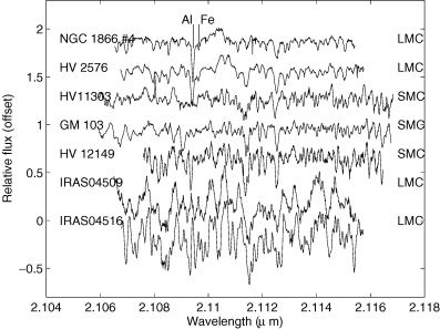
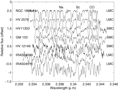
Spectra were taken of these stars using the Phoenix spectrograph (Hinkle et al. 2003) on the Gemini South telescope. The observations were done in service mode, and the observation dates are listed in Table 1. For each star, observations were made in three separate bands, as shown in Figs 1–3. First, an observation centred near 1.554 μm was made so that the OH lines could be measured for the derivation of an oxygen abundance; lines of CN also occur in this piece of spectrum. Secondly, an observation near 2.340 μm was made to measure 12CO (and possible 13CO) lines and hence the 12C abundance; given the C abundance, the CN lines near 1.554 μm then yield a 14N abundance. The Na abundance was also obtained from this spectral region. Thirdly, an observation at 2.112 μm was made to include lines of Al (and possible Mg). Lines of Fe, Sc and Ti also occur in the spectra, giving an estimate of the metal abundance.
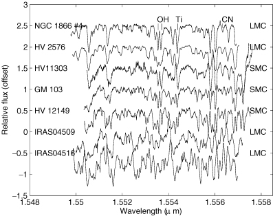
The spectra of all objects in the region near 1.554 μm. The most important lines used for abundance determination are marked.
3 PULSATION MODELS
Pulsation models and model atmospheres were made for four stars in Table 2: NGC 1866 #4, HV 2576, HV 11303 and GM 103. The spectra of the remaining stars in Table 1 (HV 12149, IRAS 04516−6902 and IRAS 04509−6922) were considered too difficult to model at this stage because of the extreme appearance of the spectra, with no clear continuum remaining (see Figs 1–3). This is presumably a result of the very large amplitude and very low effective temperatures of these stars. The J and K photometry for the four stars for which modelling was attempted is given in Table 3. Typical photometric errors are less than 0.03 mag. The J and K magnitudes have been converted to those on the AAO system of Allen & Cragg (1983) using the conversions in McGregor (1994).
The modelled stars.
| Star | L/L⊙ | Teff | M/M⊙ | ℓ/Hp | αaν |
| NGC 1866 #4 | 20 000 | 3490 | 4.0 | 2.57 | 0.05 |
| HV 2576 | 35 000 | 3350 | 6.0 | 2.21 | 0.51 |
| HV 11303 | 34 000 | 3490 | 4.6 | 2.21 | 0.58 |
| GM 103 | 41 840 | 3040 | 6.0 | 1.40 | 1.30 |
| Star | L/L⊙ | Teff | M/M⊙ | ℓ/Hp | αaν |
| NGC 1866 #4 | 20 000 | 3490 | 4.0 | 2.57 | 0.05 |
| HV 2576 | 35 000 | 3350 | 6.0 | 2.21 | 0.51 |
| HV 11303 | 34 000 | 3490 | 4.6 | 2.21 | 0.58 |
| GM 103 | 41 840 | 3040 | 6.0 | 1.40 | 1.30 |
aTurbulent viscosity parameter.
JK photometry.
| JD24a | J−K | K | JD24 | J−K | K |
| NGC 1866 #4 | HV 11303 (continued) | ||||
| 50731 | 1.23 | 9.71 | 52804 | 1.29 | 10.02 |
| 50772 | 1.27 | 9.69 | 52924 | 1.26 | 9.97 |
| 50885 | 1.24 | 9.68 | 53516 | 1.20 | 9.71 |
| 51157 | 1.30 | 9.67 | 53574 | 1.20 | 9.38 |
| 52564 | 1.29 | 9.71 | |||
| 52714 | 1.33 | 9.64 | GM 103 | ||
| 52803 | 1.25 | 9.69 | 45980 | 1.66 | 9.55 |
| 52924 | 1.28 | 9.69 | 46341 | 1.49 | 8.65 |
| 46645 | 1.54 | 8.57 | |||
| HV 2576b | 48142 | 1.63 | 9.31 | ||
| 52563 | 1.39 | 9.00 | 48168 | 1.70 | 9.23 |
| 52715 | 1.43 | 9.13 | 48640 | 1.64 | 8.36 |
| 52804 | 1.29 | 8.97 | 48851 | 1.62 | 8.78 |
| 52924 | 1.36 | 8.87 | 48934 | 1.63 | 9.13 |
| 48992 | 1.67 | 9.33 | |||
| HV 11303b,c | 49259 | 1.89 | 9.80 | ||
| 49259 | 1.19 | 9.81 | 49317 | 1.87 | 9.82 |
| 49291 | − | 9.61 | 49374 | 1.68 | 9.45 |
| 49317 | 1.17 | 9.47 | 52564 | 1.65 | 9.33 |
| 49374 | 1.19 | 9.32 | 52714 | 1.59 | 8.74 |
| 52564 | 1.21 | 9.27 | 52803 | 1.61 | 8.61 |
| 52715 | 1.39 | 9.56 | 52924 | 1.64 | 8.40 |
aJD24 is Julian Date – 2400 000. bExtra photometry is given in Wood et al. (1983). cExtra photometry is given in Catchpole & Feast (1981).
For each observed star, given estimates of the mean luminosity L and the effective temperature Teff from the J and K photometry, the stellar radius was computed from the definition L= 4πσR2T4eff. Then, given the radius and the known pulsation period, the current stellar mass was computed from the P–M–R relation of stellar pulsation. These values of mass and luminosity were then used in the non-linear pulsation calculations for the star.
The non-linear pulsation code described in Keller & Wood (2006), and references therein, was used in this study. The turbulent viscosity parameter αν was adjusted to give the observed K light-curve amplitude. The K and V magnitudes were computed using L and Teff from the pulsation models together with the bolometric corrections from Houdashelt et al. (2000a,b).
For three of the four modelled stars, MACHO light curves are available: the V magnitude was computed from the MACHO magnitude using the transforms in Bessell & Germany (1999). For the fourth star, HV 11303, an Eros2 light curve was kindly provided by Patrick Tisserand (private communication), who also provided a conversion from the two Eros2 bands to the V band. The combined V and K light curves give a V−K colour curve. The effective temperatures of the models were adjusted (by altering the ratio of mixing length to pressure scaleheight ℓ/Hp to reproduce the observed V−K colour when available, or the J−K in the one remaining case of HV 11303 (the Eros2 light curve was obtained after the modelling was completed). The final model parameters are given in Table 2. In all cases, a helium abundance Y= 0.30 was assumed, while a metal abundance Z= 0.01 was assumed for the LMC stars and Z= 0.004 was assumed for the SMC stars.
In order to construct a model atmosphere taking account of the dynamical processes in the outer layers, procedures similar to those described in Bessell, Scholz & Wood (1996), Hofmann, Scholz & Wood (1998), Scholz & Wood (2000) and Ireland et al. (2004a); Ireland, Scholz & Wood (2004b) were used, with updates to the molecular opacity from Ireland & Scholz (2006). Briefly, a pulsation model at the same pulsation phase as the phase of the Gemini observation was extracted from each pulsation series. The radial profiles of gas pressure and velocity for this model were transferred to a non-grey, spherical atmosphere code, and the temperature structure was iterated to a new state, now consistent with the atmosphere code. Once the temperature, gas pressure, density and velocity structure were all consistent in the atmosphere code, the model atmosphere structure was transferred to a separate spectrum synthesis code which was used to compute line profiles (see Section 4).
In the atmosphere code, half- and quarter-solar metal abundances from Grevesse, Noels & Sauval (1996) were adopted for LMC and SMC stars, respectively. Radiative and local thermodynamic equilibrium was adopted and, in particular, the shock-heated region behind the shock front was assumed to have negligible width and to have no effects on the temperature stratification.
The pulsation series and the extracted dynamical model used as input to the atmosphere code are now described for each star.
3.1 NGC 1866 #4
NGC 1866 #4 is the most luminous red giant in the LMC cluster NGC 1866 (the designation #4 is that given by Frogel, Mould & Blanco (1990): note that Maceroni et al. 2002 have mislabelled #4 as #2 in their paper). The MACHO light curve of this star shows a period of 158 d. Modelling the cluster Hertzsprung–Russell diagram, Brocato et al. (2003) derive masses for the He-burning giants of 3.8 –4.15 M⊙. Our derived mass for NGC 1866 #4 is 4 M⊙. With this mass and the computed mean luminosity and Teff, this star must be pulsating in the first overtone mode, a result also consistent with the small amplitude.
Fig. 4 shows the observed and computed K, V and Mbol light curves. The period and amplitude of the pulsation and the V−K colour are reproduced well. The Gemini observation was made at a phase of ∼0.1 after visual maximum. The structure of the pulsation model at this time is shown in Fig. 5. The pulsation amplitude of this star is quite small so there are no shock waves present in the atmosphere. The temperature solution from the model atmosphere program produces a cooling of the outer layers and a warming at moderate optical depths compared to the modified Eddington approximation used in the pulsation models.
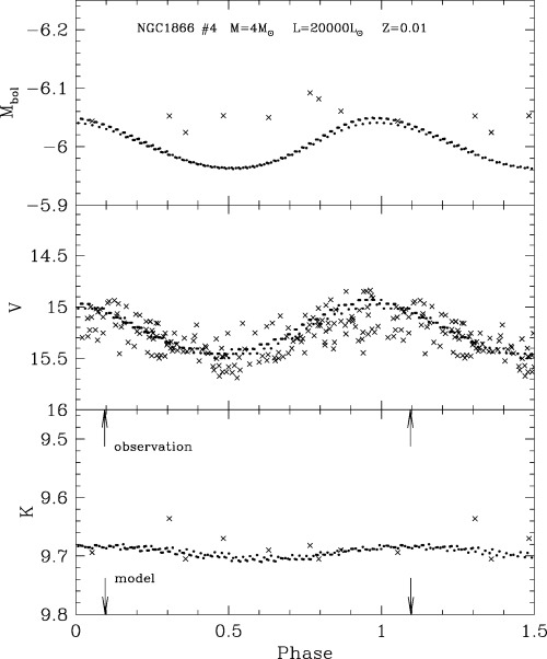
The K, V and Mbol light curves of NGC 1866 #4. The solid points are model values (several cycles are overplotted), while the crosses are observations or Mbol values computed from the J and K photometry in Table 3. The V values are computed from the MACHO MB and MR photometry using the transforms of Bessell & Germany (1999). The arrows show the phase of the Gemini observations and the phase of the pulsation model extracted for model atmosphere computation.
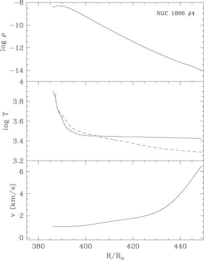
The density ρ, temperature T and velocity v plotted against radius R in a pulsation model of NGC 1866 #4 at the same phase as the phase of Gemini observation of the star. The dashed temperature profile is that obtained from the non-grey model atmosphere code.
3.2 HV 2576
HV 2576 is an LMC star which is more luminous than NGC 1866 #4. It has a much longer period, a larger amplitude and it pulsates in the fundamental mode. The derived mass for HV 2576 is 6 M⊙.
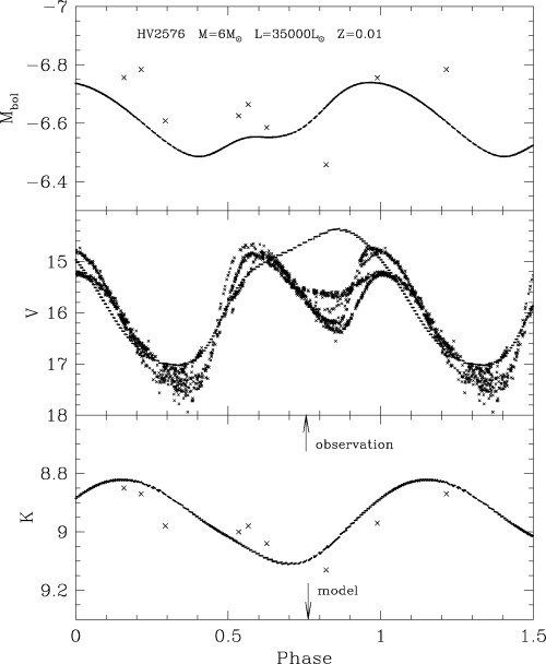
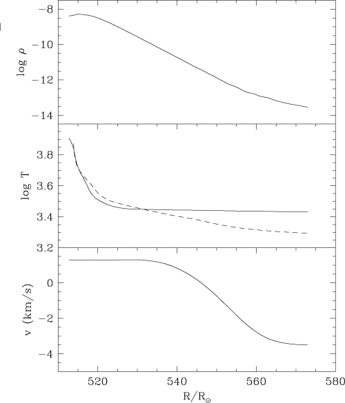
Fig. 6 shows the observed and computed K, V and Mbol light curves. Like many of the intermediate-mass, large-amplitude AGB pulsators in the Magellanic Clouds, this star shows a double-humped optical light curve. The pulsation models do not accurately reproduce the double hump but they do show some evidence for it. The K light curve does not show evidence for a prominent hump, but the points are too sparse in the light curve to be definitive. Overall, the period and amplitude of the pulsation and the large V−K colour (V−K∼ 7) are reproduced well. The Gemini observation was made near minimum light of the K light curve, or between the double-humped maximum of the optical light curve. The structure of the pulsation model at this time is shown in Fig. 7. The velocity gradient through the atmosphere at the time of observation was small and there was no shock wave present in the atmosphere. As with NGC 1866 #4, the temperature solution from the model atmosphere program produces a cooling of the outer layers and a warming at moderate optical depths compared to the modified Eddington approximation used in the pulsation models.
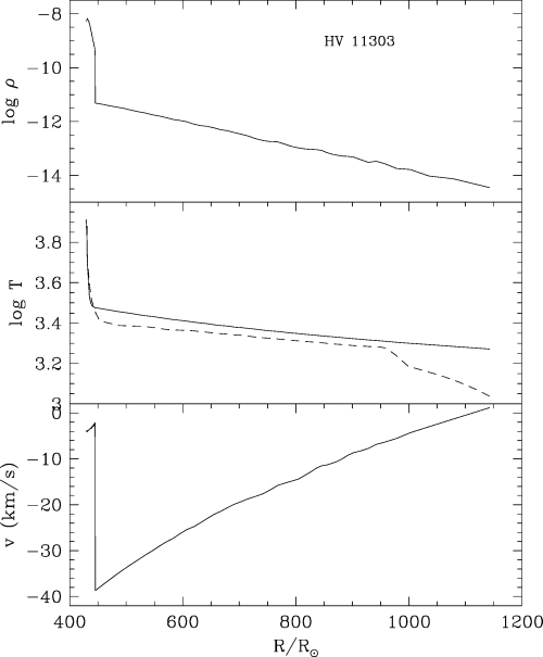
3.3 HV 11303
HV 11303 is an SMC star which is almost a twin of HV 2576 in the LMC in terms of its pulsation period and luminosity. However, it has a much larger pulsation amplitude. It pulsates in the fundamental mode and the derived mass is 4.6 M⊙. This mass is smaller than that of HV 2576, which may explain the larger pulsation amplitude.
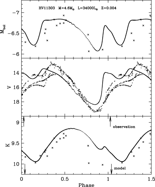
Fig. 8 shows the observed and computed K, V and Mbol light curves. The pulsation models reproduce the observed K light curve reasonably well. The Gemini observation was made near minimum light of the K light curve. The structure of the pulsation model at this time is shown in Fig. 9. Note that there is an uncertainty of about 0.1 in the phasing of the models relative to the K light curve. With the adopted phasing, a strong shock was just emerging into the atmosphere at the time of Gemini observation. In addition, there was a large velocity gradient through the atmosphere above the shock. The temperature solution from the model atmosphere program shows a large temperature drop in the outer layers. This behaviour is typical for extended atmospheres in a certain parameter range where strong water absorption abruptly dominates in the high layers (Scholz 1985). The warmer, grey pulsation model used as input to the atmosphere code does not have water-forming low temperatures.
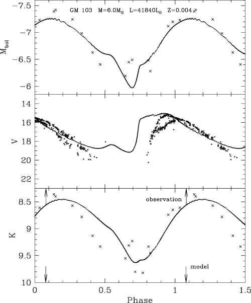
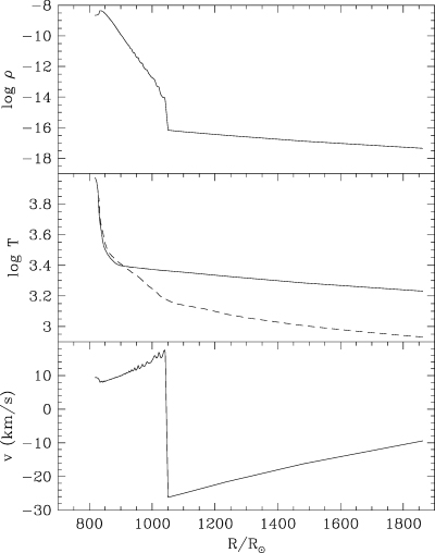
3.4 GM 103
GM 103 (Groenewegen et al. 1995) is also an SMC star but of greater luminosity, amplitude and period than HV 11303. It pulsates in the fundamental mode and the derived mass is 6 M⊙.
Fig. 10 shows the observed and computed K, V and Mbol light curves. The pulsation models reproduce the K light curve and the large V−K colour (V−K∼ 8) reasonably well. However, the V light curve of the pulsation models seems to rise towards maximum earlier than the observed light curve. The Gemini observation was made near maximum visible light, or about phase 0.1 before maximum of the K light curve. The structure of the pulsation model at this time is shown in Fig. 11. This star has a strong shock situated in the middle part of the atmosphere at the time of Gemini observation, with moderate velocity gradients above and below the shock. The temperature solution for GM 103 from the model atmosphere program shows a larger deviation from the pulsation solution than in any other star. This is due to the strong density drop at the shock, with the model atmosphere's water-dominated temperature dropping rapidly near what is the effective edge of the star at the shock front.
4 SPECTRAL SYNTHESIS AND ABUNDANCE DERIVATION
4.1 Line synthesis calculations
The spherical model atmospheres described in Section 3 were put into a compatible spectrum synthesis program (using spherical geometry) to generate line spectra. The spectrum synthesis program was that used by Scholz (1992), Bessell et al. (1996) and Scholz & Wood (2000), except that partial pressures of a larger number of molecules were calculated using a computer program supplied by K. Ohnaka (private communication). This program uses an equation of state based on molecular constants of Tsuji (1973), updated for CN using data from Costes, Naulin & Dorthe (1990) and for TiO from Tsuji (1978). Lines are assumed to be formed in local thermodynamic equilibrium. As shock heating behind the shock front is neglected in these models, emission components of synthetic line profiles may only occur as a consequence of large atmospheric extension (P-Cygni-like emission; see Scholz 1992).
The overall spectrum in each of the three filter regions was computed using a reasonably comprehensive set of atomic and diatomic molecular lines, although only specific lines were used in the actual abundance derivations. For atomic lines, wavelengths, excitation potentials and log gf values were taken from the Vienna Atomic Line Database (VALD; Kupka et al. 1999), with parameters of lines selected for abundance determination being checked against those of Smith et al. (2002). Molecular line data proved more problematic as no single source exists. CO lines were taken from Goorvitch (1994) and CN lines from Aoki & Tsuji (1997) and the SCAN data base (Jorgensen & Larsson 1990). CH lines were also obtained from the SCAN data base (Jorgensen, Larsson & Iwamae 1996). In each of these cases, lines were cross-checked against those from Smith et al. (2002). The OH lines proved most problematic. An incomplete selection of lines was assembled from Smith et al. (2002) and Meléndez, Barbay & Spite (2001): several additional lines listed in the source Abrams et al. (1994) could not be included due to a lack of gf values.
4.2 The derivation of abundances
Starting abundances were adopted by approximating LMC and SMC metal abundances as half- and quarter-solar, respectively, with solar defined from Asplund et al. (2005) (see Table 5). The CO and OH lines computed with these abundances were examined to establish the microturbulent velocity.
Derived abundances.
| Star | A(Fe) | A(12C) | A(14N) | A(16O) | A(Na) | A(Sc) | A(Ti) | A(Al) |
| LMC | ||||||||
| HV 2576 | 7.20 ± 0.10 | 7.01 ± 0.20 | 8.50 ± 0.05 | 8.28 ± 0.08 | 5.35 ± 0.10 | 2.90 ± 0.10 | 3.60 ± 0.05 | 5.50 ± 0.05 |
| NGC 1866 #4 | 7.05 ± 0.15 | 7.36 ± 0.16 | 8.55 ± 0.15 | 8.80 ± 0.17 | 5.75 ± 0.15 | 3.40 ± 0.15 | 4.70 ± 0.15 | 5.75 ± 0.10 |
| Smith et al. (2002) | 6.37–7.16 | 6.53–7.86 | 7.14–8.24 | 7.82–8.33 | 4.69–5.84 | 2.01–2.91 | 3.84–4.61 | – |
| Half-solar | 7.15 | 8.09 | 7.48 | 8.36 | 5.87 | 2.75 | 4.60 | 5.87 |
Notes: A(X) = log [n(X)/n(H)]+ 12. Half-solar abundances are half the solar abundances in Asplund et al. (2005). The errors are estimates of the line-fitting error alone – see Section 4.2.
As these relatively massive stars are expected to have altered CNO abundances as a result of nucleosynthetic processing, a series of CNO values based on the AGB evolution calculations of Karakas (2003) and Karakas & Lattanzio (2003) was adopted, and the resultant spectra were then calculated. The CNO combination giving the best overall fit to the observed spectra was used as the primary starting point for subsequent refinement of the individual CNO abundances. Once the best CNO abundances had been found, the metallic abundances were refined to give a best fit. Lines used for final abundance derivations are listed in Table 4, and a selection of the fitted lines are shown in Figs 12–25.
Spectral line data.
| λ (Å) | χ (eV) | log (gf) | Source |
| Fe i | |||
| 21 095.446 | 6.20 | −0.69 | VALD |
| Na i | |||
| 23 378.945 | 3.75 | −0.420 | Smith et al. (2002) |
| Sc i | |||
| 23 404.756 | 1.44 | −1.278 | Smith et al. (2002) |
| Ti i | |||
| 15 543.720 | 1.88 | −1.481 | Smith et al. (2002) |
| Al I | |||
| 21 093.029 | 4.09 | −0.31 | VALD |
| OH | |||
| 15 535.489 | 0.51 | −5.23 | Smith et al. (2002) |
| 15 536.707 | 0.51 | −5.23 | Meléndez et al. (2001) |
| 15 560.271 | 0.30 | −5.31 | Smith et al. (2002) |
| 15 565.815 | 0.90 | −5.00 | Meléndez et al. (2001) |
| CO | |||
| 23 396.260 | 0.37 | −5.17 | Smith et al. (2002) |
| 23 398.224 | 1.73 | −4.44 | Smith et al. (2002) |
| 23 406.345 | 0.00 | −6.57 | Smith et al. (2002) |
| 23 408.509 | 0.36 | −5.19 | Smith et al. (2002) |
| 23 424.328 | 1.80 | −4.427 | Smith et al. (2002) |
| 23 426.322 | 0.00 | −6.565 | Smith et al. (2002) |
| CN | |||
| 15 563.367 | 1.15 | −1.141 | Smith et al. (2002) |
![Fitted OH lines for HV 2576. In this and subsequent figures, fits are shown for the three abundance values shown in the figure [where A(X) = log [n(X)/n(H)]+ 12]. The dashed lines correspond to changes of ±0.15 dex from the adopted abundance (solid line).](https://oup.silverchair-cdn.com/oup/backfile/Content_public/Journal/mnras/378/3/10.1111_j.1365-2966.2007.11845.x/1/m_mnras0378-1089-f12.jpeg?Expires=1716957729&Signature=HGYfjZjKYc1P4kj~05PRGutOL8KOT5GmkI1wXgBo2HVlwNctYZu5wlANfOMp2g8Pz2pKilglxztL5YGsI6UjFcdvJSzmH5cbxGbp62NmZ52vAlnWi09M2vtR9v7UUpi4vhhOcLuCjbDUyIfzM~M3QUTbEsB~Rm3yvU-Eg3FNZsPZ5G6bomsEU1JXxGuvxV6NIOyvE-N0LjqZRJrqHE4Blha6szaPngEu7c5YHXVIF~opxP61T0YZyA2Ugw2YV8LzWoFHV5RilZpQzzA2JBb-GtiviWUoKKjELv1hi6U9l-zKb8bO33f1HfgQP8NcJRejv2UbUcN1WtDuUtALxaop1Q__&Key-Pair-Id=APKAIE5G5CRDK6RD3PGA)
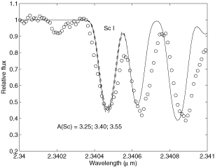
Fitted OH lines for HV 2576. In this and subsequent figures, fits are shown for the three abundance values shown in the figure [where A(X) = log [n(X)/n(H)]+ 12]. The dashed lines correspond to changes of ±0.15 dex from the adopted abundance (solid line).
Fitted OH lines for NGC 1866 #4.
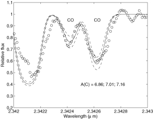
Fitted CO lines for HV 2576.

Fitted CO lines for NGC 1866 #4.
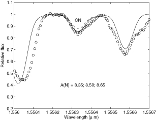
Fitted CN line for HV 2576.
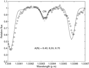
Fitted CN line for NGC 1866 #4.
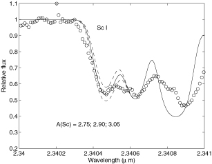
Fitted Sc i line for HV 2576.
Fitted Sc i line for NGC 1866 #4.
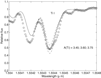
Fitted Ti i line for HV 2576.
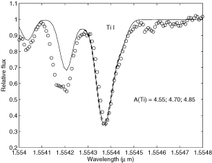
Fitted Ti i line for NGC 1866 #4.
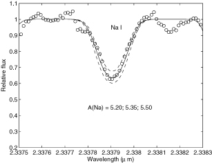
Fitted Na i line for HV 2576.
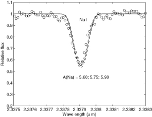
Fitted Na i line for NGC 1866 #4.
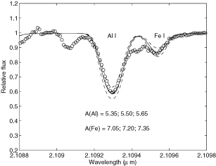
Fitted Fe i and Al lines for HV 2576.
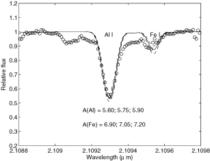
Fitted Fe i and Al lines for NGC 1866 #4.
The abundances derived from different lines of the same species show some scatter, with the adopted lines generally found to yield reasonably consistent values. Figs 14 and 15 show examples of the fit errors for the CO lines. It is clear that no CO line is fitted exactly by the final adopted abundance (that of the mean of the best fits to six lines), but both lines are fitted reasonably well, with one too strong and one too weak. Figs 12 and 13, where Fe i lines are present on either side of the OH lines, show further examples of fit errors. The adopted Fe abundance is based on a fit to the 2.1095-μm line in Figs 24 and 25. However, in HV 2576 (Fig. 12), this abundance is too high for the 1.553 424 μm Fe line to the blue and too low for the 1.553 757-μm line to the red (or, more likely, the models are missing an unidentified line at this wavelength). For NGC 1866 #4 (Fig. 13), the 1.553 424-μm line fits well, while once again the 1.553 757-μm line is too weak (or an unidentified line is missing in the model).
There were also cases where observed and computed line velocities do not match to better than a few km s−1, as can be seen in Figs 14–17. The velocity mismatch could be due to a number of potential causes, including inexact adopted line wavelengths, inexact wavelength calibration, or the model velocities as a function of depth not being correct.
The microturbulent velocity required for line broadening varied from star to star. The adopted value for NGC 1866 #4 (3 km s−1) is close to the value used by Smith et al. (2002). However, a larger value of 7 km s−1 was required for HV 2576. This value was derived by fitting to the CO lines. Slightly different values would be obtained by fitting different lines. This is probably a reflection of different amounts of turbulence at different levels in the atmosphere: the CO lines tend to be broader than the metallic lines and they are, on average, formed further out in cooler layers.
Our final derived abundances are shown in Table 5. For the elements Fe, Na, Al, Sc, Ti and N, the error estimates in the table are those arising from the fit to the line only, as only one line was available. They are eye-estimates based on the fits 0.15 dex above and below the adopted optimum fit abundance. The C and O values are based on averages of the fits to six and four lines, respectively, with the stated errors being based on the s.d. The lines used are given in Table 4. Systematic errors, such as errors in the pulsation model and its phase, will undoubtedly add significantly to the fit error, but such additional errors are hard to estimate.
4.3 HV 11303 and GM 103
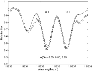
As noted in Section 3, the SMC stars HV 11303 and GM 103 both had strong shock fronts in their atmospheres at the time of observation with Gemini South. This has made abundance derivation with our atmosphere code impossible. Fig. 26 shows a sample of the spectrum for each star, along with an attempt at synthesisizing the spectrum using the pulsation models from Section 3.
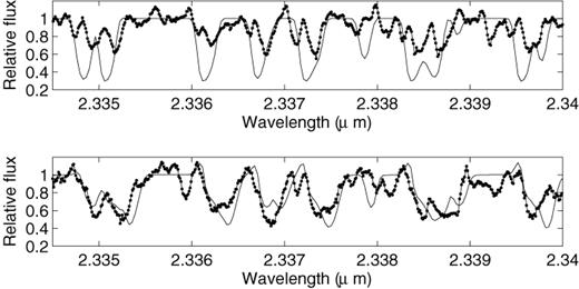
Top: A section of the 2.34-μm spectrum of GM 103 (points), overlayed with a synthesized spectrum (continuous line). Bottom: The same piece of spectrum for HV 11303.
In the case of GM 103, the synthesized absorption lines are much stronger than the observed lines. A comparison of the observed and synthesisized spectra shows clearly that the observed line cores are filled in by strong emission in every case. An alternative explanation could be that each line is split into a pre- and post-shock absorption component, with no emission in the middle. However, the weakness of the observed absorption lines compared to the model lines suggests that there is indeed a strong emission component. In HV 11303, the lines are much broader than in GM 103, with evidence for an emission component as well as absorption components corresponding to the pre- and post-shock velocities.
As noted in Section 3, the spectral synthesis code ignores the immediate post-shock, high-temperature region so that there is no post-shock emission component in our synthesized spectra. When a strong shock is present in the atmosphere, this model deficiency prevents abundance determination from lines which have a post-shock emission contribution.
These results show that observations useful for abundance analysis must be obtained at phases of the pulsation cycle when no strong shock wave is present in the atmosphere. In these relatively massive stars, the shock wave enters the lower part of the stellar atmosphere near minimum of the K light curve, or phase ∼0.2–0.3 past minimum visual light. It has passed through the line-forming part of the atmosphere half a pulsation cycle later, corresponding to ∼0.1–0.2 in phase past K maximum or after phase ∼0.4 of the visual light curve.
5 DISCUSSION
The abundances obtained here for NGC 1866 #4 and HV 2576 are shown with other comparable observations in Fig. 27. The Fe abundance is close to half-solar, consistent with the values obtained by Smith et al. (2002), Hill et al. (2000) and other studies of young objects in the LMC. The other metal abundances are similarly near half-solar, except for Ti in HV 2576 where our derived value seems anomalously low.
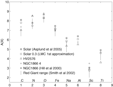
Final abundances.
The CNO abundances are the most interesting part of this study, since in a highly evolved, intermediate-mass AGB star they will be altered by the first, second and third dredge-ups and by hot-bottom burning.
Evidence for hot-bottom burning has been found in intermediate-mass AGB stars in the Magellanic Clouds by Plez, Smith & Lambert (1993) and Smith et al. (1995). Plez et al. (1993) examined spectra of seven luminous AGB stars in the SMC and found them to be Li-rich, C-poor and with low 12C/13C ratios, consistent with hot-bottom burning. Smith et al. (1995) examined a large number of SMC and LMC stars and found many luminous AGB stars, including HV 2576, showed strong Li lines that could be attributed to hot-bottom burning. In fact, HV 2576 had the largest estimated Li abundance of all the stars examined. Maceroni et al. (2002) examined Li lines in the giant stars in NGC 1866 and found that NGC 1866 #4 (which they mislabelled as #2) had enhanced Li compared to other stars in the cluster, indicating that hot-bottom burning is operating in this star also.
There is evidence that the third dredge-up has been operating in HV 2576, as well as hot-bottom burning. Wood et al. (1983) give a spectral type M5.5/S1 for HV 2576, indicating the presence of excess ZrO in the spectrum, which is a result of the dredge-up of s-process elements during thermal pulses. Smith et al. (1995) noted that HV 2576 had one of the strongest ZrO bands in their large sample of stars, indicating that a large amount of third dredge-up has occurred in this star.
The combination of third dredge-up and hot-bottom burning is predicted to be a significant source of primary nitrogen in the Universe. The 12C dredged up at a thermal pulse is converted into 14N during the next interpulse period when hot-bottom burning operates during the quiescent H-shell burning phase. Lattanzio & Wood (2004) and Karakas (2003) (see their figs 2.37 and 5.6, respectively) show the effects of third dredge-up and hot-bottom burning in intermediate-mass, luminous and subsolar metallicity AGB stars such as those we are dealing with here. Initially on the AGB, just at the onset of thermal pulses, hot-bottom burning by the CN cycle reduces the 12C abundance to ∼1/15 of its initial main-sequence value, and increases the 14N abundance to ∼5–6 times its initial value. The ratio 12C/14N at this time is ∼1/15. During subsequent evolution, the dredge-up of 12C by third dredge-up at thermal pulses, followed by hot-bottom burning, causes a steady rise over many pulsation cycles in both the C and N abundance, with the C/N ratio remaining almost constant at ∼1/15. During this relatively long evolutionary process, there is a small decrease in the O abundance, but this effect would be too small for us to reliably detect.
Looking at Fig. 27 and Table 5, we see that the C abundance in both NGC 1866 #4 and HV 2576 is about 0.1 times half-solar. At the same time, the N abundance is ∼10 times the half-solar value. Both these numbers are consistent with the strong operation of hot-bottom burning in the envelopes of these stars. Furthermore, the very large N abundances can only be explained by hot-bottom processing of dredged-up 12C into 14N, that is, a large fraction of the nitrogen in the envelopes of these stars must be of primary origin. This is the first direct demonstration that this long-predicted source of primary nitrogen does exist.
The O abundance in HV 2576 is essentially unchanged from the half-solar value, as predicted by models. There is some evidence for an increase in the O abundance in NGC 1866 #4. If confirmed, this would lend support to convective theories such as that of Herwig et al. (1997) which lead to overshoot at convective boundaries, enrichment of the intershell region in both 12C and 16O at each helium shell flash, and subsequent dredge-up of both 12C and 16O in third dredge-up events.
A strong disagreement between the observations and evolutionary models without convective overshoot relates to the total stellar mass required for the efficient operation of hot-bottom burning. The mass of NGC 1866 #4 must be no more than ∼4 M⊙ because of cluster membership. This star shows evidence for efficient hot-bottom burning, while models without convective overshoot do not predict efficient hot-bottom burning at masses this low. This suggests that overshoot (inwards) of convective material at convective boundaries is required to significantly extend the convective envelope into nuclear-burning regions. The models of Ventura, D'Antona & Mazzitelli (2002) use a convective theory that does produce overshoot, and their 4 M⊙, half-solar metal abundance AGB models do have the efficient hot-bottom burning observed in NGC 1866 #4. At 6 M⊙, both the observations of HV 2576 and models with or without convective overshoot show efficient hot-bottom burning.
The elements Li, Na and Al can also be compared with evolutionary models. Smith et al. (1995) give A(Li) = 3.8 for HV 2576 while Maceroni et al. (2002) give A(Li) = 1.5 (note that these authors used static model atmospheres, and observations at random phases where shocks may have been present in the stellar atmosphere). Models of AGB stars with efficient hot-bottom burning generally show an initial large increase in the surface Li abundance, after which it slowly decreases to low values [A(Li) ≲ 1.0] while the CN cycle converts C into N – see Karakas (2003) and Ventura et al. (2002). The high Li value derived for HV 2576, together with the observed high 14N and low 12C abundances, is consistent with model predictions for a 6 M⊙ star about one-quarter of the way through its TPAGB phase and undergoing efficient hot-bottom burning – see fig. C27 of Karakas (2003).
The Na and Al abundances found in this study are marginally below the expected half-solar values and within the expected range of observed variation. Models of AGB stars (Karakas 2003) with efficient hot-bottom burning show a small increase in Al abundance and small changes in the total Mg abundance but these are too small to detect here. The 25Mg/24Mg ratio can increase greatly in such stars, but we are unable to detect isotopic changes.
6 SUMMARY
High-dispersion, near-infrared spectra have been used to derive abundances of luminous, intermediate-mass AGB stars in the Magellanic Clouds. The C and N abundances derived here provide the first observational demonstration that third dredge-up at thermal pulses followed by hot-bottom burning can produce significant amounts of primary nitrogen in intermediate-mass AGB stars. The observed spectra and modelling show that only spectra taken during the part of the pulsation cycle near minimum visual light, equivalent to the latter part of the decline of the K light curve, are useful for abundance analysis.
The results in this paper come from exploratory observations and calculations and, in the end, only two stars were suitable for abundance analysis. It is clear that follow-up work with a larger sample of objects is required to confirm the results found here, and to seek C and N abundances as a function of stellar mass, luminosity and metal abundance.
We would like to thank Amanda Karakas for useful discussions about AGB nucleosynthesis models, Patrick Tisserand for supplying the Eros2 light curve for HV 11303, and Keiichi Ohnaka for supplying his programs for partial pressure calculations. JAM is grateful for the discovery grant from the Australian Research Council (DP0343832) which supported her during the course of this work: PRW and JCL also received partial support from this grant. MS received support from a grant of the Deutsche Forschungsgemeinschaft. This paper is based in part on observations obtained at the Gemini Observatory, which is operated by the Association of Universities for Research in Astronomy, Inc., under a cooperative agreement with the NSF on behalf of the Gemini partnership: the National Science Foundation (United States), the Particle Physics and Astronomy Research Council (United Kingdom), the National Research Council (Canada), CONICYT (Chile), the Australian Research Council (Australia), CNPq (Brazil) and CONICRT (Argentina). The observations were obtained with the Phoenix infrared spectrograph, which was developed and is operated by the National Optical Astronomy Observatory. The spectra were obtained as part of Gemini programmes GS-2002A-Q-49, GS-2002B-Q-22 and GS-2003A-Q-25. We thank the observers at Gemini South for taking these spectra in service mode.
REFERENCES
