


Abstract
The antisymmetrized quasi-cluster model (AQCM) was proposed to describe |$\alpha$|-cluster and |$jj$|-coupling shell models on the same footing. In this model, the cluster–shell transition is characterized by two parameters, |$R$| representing the distance between |$\alpha$| clusters and |$\varLambda$| describing the breaking of |$\alpha$| clusters, and the contribution of the spin–orbit interaction, very important in the |$jj$|-coupling shell model, can be taken into account starting with the |$\alpha$|-cluster model wave function. Not only the closure configurations of the major shells but also the subclosure configurations of the |$jj$|-coupling shell model can be described starting with the |$\alpha$|-cluster model wave functions; however, the particle–hole excitations of single particles have not been fully established yet. In this study we show that the framework of AQCM can be extended even to the states with the character of single-particle excitations. For |$^{12}\mathrm{C}$|, two-particle–two-hole (2p2h) excitations from the subclosure configuration of |$0p_{3/2}$| corresponding to a BCS-like pairing are described, and these shell model states are coupled with the three |$\alpha$|-cluster model wave functions. The correlation energy from the optimal configuration can be estimated not only in the cluster part but also in the shell model part. We try to pave the way to establish a generalized description of the nuclear structure.
1. Introduction
One of the important goals of nuclear structure physics is the description of both shell and cluster aspects on the same footing. Real nuclear systems have characteristics of both aspects, and the mixing or competition between these two is an important subject for the physics of quantum many-body systems [1-3]. Our strategy is to establish a framework, which starts with the cluster model side, in contrast with standard approaches, and includes shell correlations.
As it is well known, when we take zero limit for the relative distances between clusters, the model space coincides with that of the lowest shell model configuration. This is called the SU(3) limit [4,5], and for |$N=Z$| nuclei with magic numbers of a 3D harmonic oscillator (|$N=Z=2,8,20,\ldots$|), the cluster model wave functions agree with the doubly closed shell configurations. Here both spin–orbit favored (|$j$|-upper) and unfavored (|$j$|-lower) single-particle orbits are filled and we can forget about the spin–orbit contribution. However, the spin–orbit effect exists in other cases, and in most of the conventional cluster models, this effect cannot be taken into account; the spin–orbit contribution cancels because of the assumption of the |$\alpha$| cluster that four nucleons have the same form of the spatial wave function.
To overcome this difficulty with the cluster model, we proposed an antisymmetrized quasi-cluster model (AQCM) [2,3,6–11], which enables us to describe the |$jj$|-coupling shell model states with the spin–orbit contribution starting with the cluster model wave function. In AQCM, the transition from the cluster- to the shell-model structure can be described by two parameters; |$R$| representing the distance between |$\alpha$| clusters, and |$\varLambda$|, which characterizes the transition of |$\alpha$| cluster(s) to quasi-cluster(s) and quantifies the role of the spin–orbit interaction. In Ref. [2], the AQCM wave function was shown to correspond to the |$(0s_{1/2})^4 (0p_{3/2})^8$| closed shell configuration of |$^{12}\mathrm{C}$|, and the strong contribution of the spin–orbit interaction was taken into account. The optimal ground state of |$^{12}\mathrm{C}$| was shown to have an intermediate character between the three |$\alpha$| clusters and shell model states. In a similar way, the subclosure configuration of |$0d_{5/2}$| was described in |$^{28}\mathrm{Si}$|, and characteristic magic numbers of the |$jj$|-coupling shell model, |$28$| and |$50$|, were successfully described in |$^{56}\mathrm{Ni}$| and |$^{100}\mathrm{Sn}$| [10].
However, the particle–hole excitations of single particles are not yet fully established from a cluster model point of view. The purpose of the present study is to show that the framework of AQCM can be extended even to the states with the character of single-particle excitations. The first example is |$^{12}\mathrm{C}$|. In this paper, we prepare two different models and perform a variational calculation. One is the cluster model; we prepare three |$\alpha$|-cluster states, which give almost converged energy for the ground state and the second |$0^+$| state, but this is only within the isosceles triangular configurations. The other one is the |$jj$|-coupling shell model, which is prepared by using AQCM. In addition, we can prepare the states corresponding to the 2p2h excitation of the |$jj$|-coupling shell model using AQCM. The |$jj$|-coupling shell model is in principle a complete set, and we have to limit the model space. Here we focus on the time reversal excitation of two particles, which corresponds to the BCS-like parings of proton–proton, neutron–neutron, and proton–neutron. We discuss the competition between normal pairing and proton–neutron pairing effects.
So far the features of |$^{12}\mathrm{C}$| have been investigated using many different models; various cluster models [12-14], shell models including modern ab initio ones [15,16], and so on. The |$0_2^+$| state, which is known as the Hoyle state, is nicely described by the three |$\alpha$|-cluster models; however, they cannot describe detailed properties related to the |$\alpha$|-cluster breaking effect, especially in the ground state rotational band. On the other hand, in principle the shell model provides a complete set, but the cluster states are in practice difficult to describe within finite model space. Takigawa et al. have introduced a hybrid model to mix the |$\alpha$|-cluster model and |$p$| shell SU(3) basis states [17]. Our concept is based on this idea; however, we transform the cluster model wave functions directly into those of the |$jj$|-coupling shell model and try to pave the way to establish a generalized description of the nuclear structure. Also, antisymmetrized molecular dynamics (AMD) and fermionic molecular dynamics (FMD) have been successfully introduced to describe both characters of shell and cluster models [18-22]. In these models, the central positions of all the nucleons are optimized under some constraints. On the other hand, in our approach, we introduce much fewer and more controllable parameters, which allow the description of excited configurations.
Concerning the universal description of the nuclear structure, the philosophy of the present study has some similarity to that of Wildermuth and Tang [23]. There, harmonic oscillator shell model states (SU(3) states) are generated from the |$\alpha$|-cluster model. There are some technical similarities between this work and our AQCM; an imaginary part is introduced to express the boost of the nucleons, and a stretched configuration of the spherical harmonics is used to simplify the discussion. However, we do not only study harmonic oscillator shell model states; we further describe |$jj$|-coupling shell model states starting with the |$\alpha$|-cluster model, and the breaking effect of the clusters can be discussed.
In AQCM, we transform a Brink-type |$\alpha$|-cluster model wave function [24] into the |$jj$|-coupling shell model wave function by giving an imaginary part for the Gaussian center parameters. This procedure has some similarity to the idea of Fock–Bargmann space developed by Filippov et al. [25]. In Ref. [25], they discussed |$^6\mathrm{He}$|, introduced hyperspherical harmonics basis states for the description of two valence neutrons outside of the |$\alpha$| core, and extracted the matrix elements of the Hamiltonian from the expectation value obtained by using a Gaussian wave packet. We also use Gaussian wave packets; however, in our study, we directly transform the wave function into the |$jj$|-coupling shell model and the breaking effect of the |$\alpha$|-cluster part can be discussed.
In |$^{12}$|C, the presence of |$D_{3h}$| symmetry, which reflects the equilateral triangular symmetry of three |$\alpha$| clusters, was recently confirmed [26]. When a system has this symmetry, both |$K^\pi = 0^+$| and |$3^-$| rotational bands are possible, and recently these bands were experimentally confirmed. All the observed states in the low-lying region of |$^{12}$|C are well described by the algebraic cluster model [27–29]. In addition, tetrahedral symmetry of four |$\alpha$| clusters is discussed in |$^{16}$|O based on this model [30]. Although the model space and the symmetry of the wave function are slightly different, our approach is expected to be a complementary one to the algebraic cluster model.
This paper is organized as follows. We describe our formulation in this work including the review of AQCM in Sect. 2. The results and discussion are given in Sect. 3. Finally, we present the conclusion and outlook in Sect. 4.
2. Formulation
2.1. AQCM wave function
As in many conventional models, the single-particle wave function of AQCM (|$\phi_i$|) consists of spatial (|$\psi_i$|), spin (|$\chi_i$|), and isospin (|$\tau_i$|) parts:
The spatial part of the single-particle wave function has a Gaussian shape [24],
2.2. Description of subclosure configuration |$(^{12}\mathrm{C}$| case|$)$|
2.3. Extension of AQCM
Here we explain our new model, which is the extension of AQCM.
2.3.1. Total wave function
For the basis states, we prepare both the shell and cluster model ones. For the shell model part, we use AQCM, and in addition to the subclosure configuration of |$0p_{3/2}$|, we introduce five different two-particle–two-hole (2p2h) configurations. For the cluster model space, we introduce thirty different three-|$\alpha$| configurations. In total, we superpose |$6+30=36$| basis states and diagonalize the Hamiltonian. For the width parameter |$\nu$||$(=1/2b^2)$| in Eq. (2), we take |$b=1.4\,\mathrm{fm}$|.
For the shell model basis states, as shown in the previous subsection, we can transform the |$\alpha$|-cluster model wave function to the |$0p_{3/2}$| subclosure configuration of the |$jj$|-coupling shell model using AQCM. This is |$(0s_{1/2})^2(0p_{3/2})^4$| for the proton and neutron parts, and here we call it the zero-particle–zero-hole (0p0h) state. To generate this state, we take a small enough |$R$| value of |$R=0.1\,\mathrm{fm}$| in Eqs. (4) and (5). In addition, we introduce five 2p2h configurations. Four of them correspond to the normal BCS-like pairing effect of protons or neutrons; |$(0s_{1/2})^2(0p_{3/2})^2(0p_{1/2})^2$| and |$(0s_{1/2})^2(0p_{3/2})^2(0d_{5/2})^2$| are introduced for the proton part or neutron part. We further take into account the proton–neutron pairing effect. For this purpose, we prepare a basis state, where one proton and one neutron are excited from |$0p_{3/2}$| to |$0p_{1/2}$|; |$(0s_{1/2})^2(0p_{3/2})^3(0p_{1/2})^1$| for both proton and neutron parts. This is also 2p2h, but each isospin (proton or neutron) part is one-particle–one-hole (1p1h). In total we introduce six configurations for the |$0^+$| states of |$^{12}\mathrm{C}$|; 0p0h for both proton and neutron parts (|$pn$|–0p0h), 2p2h excitation to |$0p_{1/2}$| for the proton part (|$pp$|–|$p_{1/2}$|–2p2h), that for the neutron part (|$nn$|–|$p_{1/2}$|–2p2h), 2p2h excitation to |$0d_{5/2}$| for the proton part (|$pp$|–|$d_{5/2}$|–2p2h), that for the neutron part (|$nn$|–|$d_{5/2}$|–2p2h), and 1p1h to |$0p_{1/2}$| for both proton and neutron parts (|$pn$|–|$p_{1/2}$|–2p2h). The 1p1h configuration is explained in Sect. 3.3, and the 2p2h configurations are explained in Sects. 3.2 and 3.4.
For the cluster model basis states, as schematically shown in Fig. 1, the configurations are introduced with isosceles triangular shapes. The parameters |$d$| and |$h$| are the base and height of the isosceles triangle, respectively, and they are taken as |$d=1,2,\ldots,5\,\mathrm{fm}$| and |$h=1,2,\ldots,6\,\mathrm{fm}$|. There are |$5\times6=30$| basis states for the cluster model side.
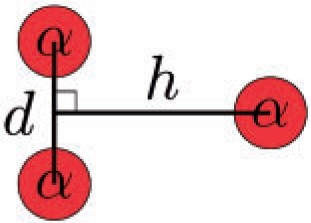
Schematic figure for the cluster model configurations. The red spheres show the |$\alpha$| clusters.
2.3.2. Hamiltonian
3. Results and discussion
As already seen, the closure configurations of the major shells can be described by conventional |$\alpha$|-cluster models, and subclosure configurations of the |$jj$|-coupling shell model can be described by AQCM. Here we extend AQCM. First we discuss the AQCM wave functions with general |$\varLambda$| values and next show how to describe particle–hole excitations. For |$^{12}\mathrm{C}$|, single-particle excitations from |$0p_{3/2}$| to |$0p_{1/2}$| and |$0d_{5/2}$| are introduced for the proton part, neutron part, and proton–neutron part, and the effect of BCS-like pairing is incorporated. Finally these shell-model-like wave functions are coupled with the three |$\alpha$|-cluster wave functions.
3.1. AQCM wave functions with general |$\varLambda$| values
We have already discussed that |$\varLambda = 0$| corresponds to |$\alpha$|-cluster states and |$\varLambda=1$| with small |$R$| corresponds to the |$jj$|-coupling shell model states. However, the discussion for general |$\varLambda$| values (|$\varLambda\neq 0,1$|) is insufficient. In this subsection, we investigate the feature of the AQCM wave functions with general |$\varLambda$| values in |$^{12}\mathrm{C}$|.
The single-particle wave functions of protons |$i=3$|–6 are generated by multiplying the rotational operators |$\hat{R}(0,2\pi/3,0)$| or |$\hat{R}(0,4\pi/3,0)$| for the single-particle wave functions of protons |$i=1,2$| as in the original AQCM [2]:
3.2. Description of 2p2h |$(p_{1/2}-2p2h$)$|
3.3. Description of 1p1h
Now a proton has all six components of |$0p$| orbits, and we remove some of them by imposing conditions. If |$A_i\sin(\beta_i/2)-\sqrt{2}C_i\cos(\beta_i/2)=0$| is satisfied, we can eliminate the component of |$|p,3/2,1/2\rangle$|. Similarly, if |$C_i\sin(\beta_i/2)-\sqrt{2}B_i\cos(\beta_i/2)=0$| is satisfied, the component of |$|p,1/2,-1/2\rangle$| vanishes. Thus, if |$A_i\sin(\beta_i/2)-\sqrt{2}C_i\cos(\beta_i/2)=0$| and |$C_i\sin(\beta_i/2)-\sqrt{2}B_i\cos(\beta_i/2)=0$| are simultaneously satisfied, the single-particle wave function does not have the |$|p,3/2,1/2\rangle$| and |$|p,1/2,-1/2\rangle$| components. This was for one proton; however, if all the protons satisfy the same conditions, the proton part of the wave function also does not have the components of |$|p,3/2,1/2\rangle$| and |$|p,1/2,-1/2\rangle$|. This is nothing but 1p1h excitation to |$0p_{1/2}$|.
In the following part, we simplify the conditions to describe 1p1h. The conditions |$A_i\sin(\beta_i/2)-\sqrt{2}C_i\cos(\beta_i/2)=0$| and |$C_i\sin(\beta_i/2)-\sqrt{2}B_i\cos(\beta_i/2)=0$| are equivalent to |$\tan(\beta_i/2)=\sqrt{2}C_i/A_i=\sqrt{2}B_i/C_i$|. Substituting |$A_i=(a_i+b_i)/2$|, |$B_i=(a_i-b_i)/2$|, and |$C_i=c_i/\sqrt{2}$|, the conditions become |$a_i^2-b_i^2=2c_i^2$|. As |$a_i$|, |$b_i$|, and |$c_i$| are real numbers, another condition of |$|a_i|\ge|b_i|$| is required. As a result, the conditions for the spin part of the wave function become |$\tan(\beta_i/2)=\mathrm{sign}(a_ic_i)\sqrt{2(a_i-b_i)/(a_i+b_i)}$|, where |$\mathrm{sign}(\xi)=\xi/|\xi|$|. As an example that realizes the conditions |$a_i^2-b_i^2=2c_i^2$| and |$\tan(\beta_i/2)=\mathrm{sign}(a_ic_i)\sqrt{2(a_i-b_i)/(a_i+b_i)}$|, we show a set for the six protons in Table 1. The center of mass of the system is set to the origin. The parameters for protons |$i=1$| and |$2$| are equivalent to the ones for the original AQCM wave function [2]. We can confirm that the presence of a real parameter |$\varLambda$| avoids the risk that some of the single-particle orbits are not linearly independent. For the range of |$\varLambda$|, only |$0<\varLambda<1$| is allowable. Using these parameters, the wave function of the proton part |$\varPsi_p=\mathcal{A}[\phi_1,\ldots,\phi_6]$| describes the |$(0s_{1/2})^2(0p_{3/2})^3(0p_{1/2})^1$| configuration at the limit of |$R\to0$|.
Example of |$\{(a_i,ib_i,c_i)\}$| and coefficients for the spin wave functions for the six protons (|$i=$|1–6), which describes the 1p1h configuration. The required conditions are |$a_i^2-b_i^2=2c_i^2$| and |$\tan(\beta_i/2)=\mathrm{sign}(a_ic_i)\sqrt{2(a_i-b_i)/(a_i+b_i)}$|. The center of mass of the system is set to the origin. The parameters |$a_i$|, |$b_i$|, and |$c_i$| are introduced in Eq. (40), and the parameter |$\beta_i$| is introduced in Eq. (41).
| i | 1 | 2 | 3 | 4 | 5 | 6 |
|---|---|---|---|---|---|---|
| |$a_i$| | |$1$| | |$1$| | |$-\frac{1}{2}$| | |$-\frac{1}{2}$| | |$-\frac{1}{2}$| | |$-\frac{1}{2}$| |
| |$ib_i$| | |$i$| | |$-i$| | |$\frac{1}{2}i\varLambda$| | |$-\frac{1}{2}i\varLambda$| | |$\frac{1}{2}i\varLambda$| | |$-\frac{1}{2}i\varLambda$| |
| |$c_i$| | |$0$| | |$0$| | |$\frac{\sqrt{1-\varLambda^2}}{2\sqrt{2}}$| | |$\frac{\sqrt{1-\varLambda^2}}{2\sqrt{2}}$| | |$-\frac{\sqrt{1-\varLambda^2}}{2\sqrt{2}}$| | |$-\frac{\sqrt{1-\varLambda^2}}{2\sqrt{2}}$| |
| coefficient for |$\chi_\uparrow$| (|$\cos\frac{\beta_i}{2}$|) | |$1$| | |$0$| | |$\sqrt{\frac{1-\varLambda}{3+\varLambda}}$| | |$\sqrt{\frac{1+\varLambda}{3-\varLambda}}$| | |$\sqrt{\frac{1-\varLambda}{3+\varLambda}}$| | |$\sqrt{\frac{1+\varLambda}{3-\varLambda}}$| |
| coefficient for |$\chi_\downarrow$| (|$\sin\frac{\beta_i}{2}$|) | |$0$| | |$1$| | |$-\sqrt{2}\sqrt{\frac{1+\varLambda}{3+\varLambda}}$| | |$-\sqrt{2}\sqrt{\frac{1-\varLambda}{3-\varLambda}}$| | |$\sqrt{2}\sqrt{\frac{1+\varLambda}{3+\varLambda}}$| | |$\sqrt{2}\sqrt{\frac{1-\varLambda}{3-\varLambda}}$| |
The conditions that eliminate the components of |$|p,3/2,-1/2\rangle$| and |$|p,1/2,1/2\rangle$| in Eq. (43) are |$\sqrt{2}C_i\sin(\beta_i/2)+B_i\cos(\beta_i/2)=0$| and |$\sqrt{2}A_i\sin(\beta_i/2)+C_i\cos(\beta_i/2)=0$|. These conditions are equivalent to |$a_i^2-b_i^2=2c_i^2$| and |$\tan(\beta_i/2)=-\mathrm{sign}(a_ic_i)\sqrt{(a_i-b_i)/[2(a_i+b_i)]}$|. As an example that satisfies these conditions, we show a set of |$\{(a_i,ib_i,c_i)\}$| and coefficients for the spin wave functions for the six neutrons in Table 2. The center of mass of the system is set to the origin. We choose these parameters in Table 2 for the neutron part.
Example of |$\{(a_i,ib_i,c_i)\}$| and coefficients for the spin wave functions for the six neutrons (|$i=7$|–12), which describes the 1p1h configuration. The required conditions are |$a_i^2-b_i^2=2c_i^2$| and |$\tan(\beta_i/2)=-\mathrm{sign}(a_ic_i)\sqrt{(a_i-b_i)/[2(a_i+b_i)]}$|. The center of mass of the system is set to the origin. The parameters |$a_i$|, |$b_i$|, and |$c_i$| are introduced in Eq. (40), and the parameter |$\beta_i$| is introduced in Eq. (41).
| i | 7 | 8 | 9 | 10 | 11 | 12 |
|---|---|---|---|---|---|---|
| |$a_i$| | |$1$| | |$1$| | |$-\frac{1}{2}$| | |$-\frac{1}{2}$| | |$-\frac{1}{2}$| | |$-\frac{1}{2}$| |
| |$ib_i$| | |$i$| | |$-i$| | |$\frac{1}{2}i\varLambda$| | |$-\frac{1}{2}i\varLambda$| | |$\frac{1}{2}i\varLambda$| | |$-\frac{1}{2}i\varLambda$| |
| |$c_i$| | |$0$| | |$0$| | |$\frac{\sqrt{1-\varLambda^2}}{2\sqrt{2}}$| | |$\frac{\sqrt{1-\varLambda^2}}{2\sqrt{2}}$| | |$-\frac{\sqrt{1-\varLambda^2}}{2\sqrt{2}}$| | |$-\frac{\sqrt{1-\varLambda^2}}{2\sqrt{2}}$| |
| coefficient for |$\chi_\uparrow$| (|$\cos\frac{\beta_i}{2}$|) | |$1$| | |$0$| | |$\sqrt{2}\sqrt{\frac{1-\varLambda}{3-\varLambda}}$| | |$\sqrt{2}\sqrt{\frac{1+\varLambda}{3+\varLambda}}$| | |$\sqrt{2}\sqrt{\frac{1-\varLambda}{3-\varLambda}}$| | |$\sqrt{2}\sqrt{\frac{1+\varLambda}{3+\varLambda}}$| |
| coefficient for |$\chi_\downarrow$| (|$\sin\frac{\beta_i}{2}$|) | |$0$| | |$1$| | |$\sqrt{\frac{1+\varLambda}{3-\varLambda}}$| | |$\sqrt{\frac{1-\varLambda}{3+\varLambda}}$| | |$-\sqrt{\frac{1+\varLambda}{3-\varLambda}}$| | |$-\sqrt{\frac{1-\varLambda}{3+\varLambda}}$| |
3.4. Description of |$(0s_{1/2})^2(0p_{3/2})^2(0d_{5/2})^2$| configuration |$(d_{5/2}$|–2p2h|$)$|
3.4.1. Description of |$(0s_{1/2})^2(0p_{3/2})^2(0d_{5/2})^2$| configuration by a linear structure
3.4.2. Description of |$(0s_{1/2})^2(0p_{3/2})^2(0d_{5/2})^2$| configuration by a regular triangle structure
3.5. Energy levels and principal quantum numbers
We couple all of the 2p2h configurations to the subclosure configuration of |$0p_{3/2}$|, and finally the three |$\alpha$|-cluster wave functions are mixed. Concerning the |$R$| and |$\varLambda $| values, for the 1p1h configuration in Sect. 3.3, |$R=0.1\,\mathrm{fm}$| and |$\varLambda=0.1$| are employed, and for the 2p2h excitation to |$0p_{1/2}$| in Sect. 3.2, we take |$R=0.1\,\mathrm{fm}$| and |$(\varLambda_a,\varLambda_b)=(-3/2,0)$|. For the 2p2h excitation to |$0d_{5/2}$| in Sect. 3.4, we take |$R=0.1\,\mathrm{fm}$| in Eqs. (4) and (5). We discuss the obtained |$0^+$| energy levels, principal quantum numbers, and |$E0$| transition matrix elements.
3.5.1. Energy levels with the shell model basis states
We start with the shell model configurations introduced in Sect. 2.3. Figure 2(a) shows the |$0^+$| energy of |$^{12}\mathrm{C}$| with the subclosure configuration of |$0p_{3/2}$| (|$pn$|–0p0h), which is |$-84.5\,\mathrm{MeV}$| (the experimental value is |$-92.2\,\mathrm{MeV}$| [33]). In Fig. 2(b), the |$0^+$| levels obtained after coupling with the 2p2h configurations are shown. Here, we mixed five different 2p2h configurations; two nucleons are excited from |$0p_{3/2}$| to |$0p_{1/2}$| (|$pp$|–|$p_{1/2}$|–2p2h, |$nn$|–|$p_{1/2}$|–2p2h), or they are excited to |$0d_{5/2}$| (|$pp$|–|$d_{5/2}$|–2p2h, |$nn$|–|$d_{5/2}$|–2p2h). In addition, we couple a configuration that one proton and one neutron are excited from |$0p_{3/2}$| to |$0p_{1/2}$| (|$pn$|–|$p_{1/2}$|–2p2h). In this way, we include the effects of BCS-like pairing for the proton part, neutron part, and proton–neutron part. The energy of the ground state becomes |$-86.9\,\mathrm{MeV}$|, and this is lower than that of the subclosure configuration by |$2.4\,\mathrm{MeV}$|. The reduction is caused by the coherent effects of the three BCS-like pairings. The squared overlap between the ground state of the shell-model basis states and subclosure configuration of |$0p_{3/2}$| (|$pn$|–0p0h) is |$0.91$|.
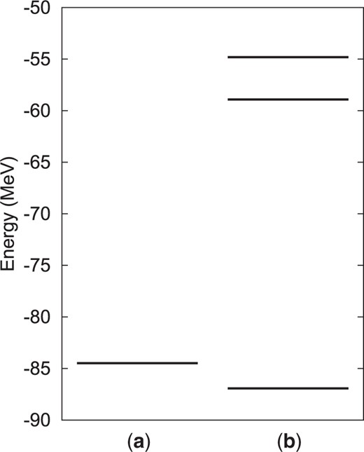
|$0^+$| energy levels of |$^{12}\mathrm{C}$| calculated with shell model-like basis states. (a) |$0^+$| energy of the subclosure configuration of |$0p_{3/2}$| (|$pn$|–0p0h), (b) |$0^+$| levels obtained after coupling with the 2p2h states.
3.5.2. Competition of shell and cluster structures
Finally we couple the shell and cluster basis states. In Table 3, the |$0^+$| energies (|$E\,(\mathrm{MeV})$|) and principle quantum numbers (|$N$|) of |$^{12}\mathrm{C}$| are shown. The present interaction gives a slightly lower ground state energy for the cluster basis states (|$-89.1\,\mathrm{MeV}$|) compared with the one for the shell model basis states (|$-86.9\,\mathrm{MeV}$|), but this is related to the fine tuning of the interaction parameters. The ground state energy is reduced by |$3.5\,\mathrm{MeV}$| from the one for the cluster model basis states by mixing both the shell and cluster model basis states (|$-92.6\,\mathrm{MeV}$|), since the spin–orbit interaction was not taken into account within the cluster model basis states. If we calculate without the 2p2h basis states, namely only within the subclosure configuration of |$0p_{3/2}$| and cluster model basis states, the energy is |$-91.8\,\mathrm{MeV}$|. This is higher by |$0.8\,\mathrm{MeV}$| than the final result, and the mixing of the 2p2h configurations is found to have a certain effect. The principal quantum number for the ground state obtained with the shell model basis states is close to |$8$|, which is the lowest possible value, even though 2p2h excitations to |$0d_{5/2}$| are allowed. On the other hand, the cluster model gives a rather large value of |$11.22$|, and this is reduced to |$9.15$| after coupling with the shell model basis states. The three-|$\alpha$| configuration shrinks after coupling with the |$jj$|-coupling shell model states, as discussed in many preceding works including ours [3,18,19,21].
|$0^+$| energies (|$E\,(\mathrm{MeV})$|) and principle quantum numbers (|$N$|) of |$^{12}\mathrm{C}$| calculated using the shell (shell), cluster (cluster) model basis states. The values for the mixed model space, subclosure configuration of |$0p_{3/2}$|, and cluster model basis states are shown in the column “|$pn$|–0p0h+cluster”. The values for the full model space, shell, and cluster basis states are shown in the column “shell+cluster”.
| shell | cluster | |$pn$|–0p0h+cluster | shell+cluster | |||||
|---|---|---|---|---|---|---|---|---|
| |$E$| | |$N$| | |$E$| | |$N$| | |$E$| | |$N$| | |$E$| | |$N$| | |
| |$0_1^+$| | |$-86.9$| | |$8.00$| | |$-89.1$| | |$11.22$| | |$-91.8$| | |$\ \, 9.40$| | |$-92.6$| | |$\ \, 9.15$| |
| |$0_2^+$| | |$-58.9$| | |$8.01$| | |$-79.1$| | |$20.01$| | |$-83.2$| | |$13.82$| | |$-83.4$| | |$14.00$| |
The |$0_2^+$| state is the famous Hoyle state, which has the character of three |$\alpha$| clusters. Experimentally the state appears at |$E_x = 7.65\,\mathrm{MeV}$|, and our final result gives |$9.2\,\mathrm{MeV}$|. Within the cluster model basis states only, the principal quantum number is |$20.01$|, and this is reduced to |$14.00$| after coupling with the shell model basis states. Since the ground state wave function is drastically changed after mixing the shell model basis states with the cluster configurations, the |$0_2^+$| state is also influenced because of the orthogonal condition [34]. The matrix element of the |$E0$| transition between the |$0_1^+$| and |$0_2^+$| states is |$7.36\,e\,\mathrm{fm}^2$|, which is |$9.22\,e\,\mathrm{fm}^2$| within the cluster model basis states only (the experimental value is |$5.52\,e\,\mathrm{fm}^2$|).
In Table 4, we show the squared overlaps between the |$0_{1,2}^+$| states obtained with the full model space and the six shell model basis states introduced in the calculation. The squared overlap between the |$0_1^+$| state and the |$pn$|–0p0h is |$0.42$|, which is reduced from the one within the shell model basis states only (|$0.91$|). This is because, using the present interaction parameters, the cluster model basis states give a lower ground state energy compared with the shell model basis states; however, this tendency may change when we use a slightly different parameter set. Concerning the 2p2h configurations, the squared overlaps between the |$0_1^+$| state and |$pn$|–, |$pp$|–, and |$nn$|–|$p_{1/2}$|–2p2h are about 0.04–0.07, which are not negligible. However, the squared overlap between the |$0_1^+$| state and |$pp$|–|$d_{5/2}$|–2p2h or |$nn$|–|$d_{5/2}$|–2p2h is more than an order of magnitude smaller. For the |$0_2^+$| state, it has a squared overlap with |$pn$|–0p0h of |$0.33$|, but the squared overlaps with the 2p2h configurations are quite small. Note that for each |$0^+$| state, the sum these squared overlaps does not become unity. This is because the solution of our model contains both cluster model space and |$jj$|-coupling shell model space. The cluster model and |$jj$|-coupling shell model have some overlap, but they are different. The values in this table are just the projection to the |$jj$|-coupling shell model space, and the remaining part is the contribution of the cluster states.
Squared overlaps between the |$0_{1,2}^+$| states and the six shell model basis states.
| |$pn$|–0p0h | |$pn$|–|$p_{1/2}$|–2p2h | |$pp$|–|$p_{1/2}$|–2p2h | |$nn$|–|$p_{1/2}$|–2p2h | |$pp$|–|$d_{5/2}$|–2p2h | |$nn$|–|$d_{5/2}$|–2p2h | |
|---|---|---|---|---|---|---|
| |$0_1^+$| | |$4.21\times10^{-1}$| | |$3.96\times10^{-2}$| | |$6.78\times10^{-2}$| | |$6.86\times10^{-2}$| | |$9.26\times10^{-4}$| | |$9.64\times10^{-4}$| |
| |$0_2^+$| | |$3.28\times10^{-1}$| | |$1.10\times10^{-4}$| | |$4.30\times10^{-4}$| | |$5.27\times10^{-4}$| | |$8.41\times10^{-4}$| | |$7.92\times10^{-4}$| |
4. Conclusion
We have developed the framework of AQCM to describe not only the subclosure configuration of the |$jj$|-coupling shell model but also the 2p2h configurations, in addition to the cluster model wave functions. In |$^{12}\mathrm{C}$|, it was shown that the 2p2h excitations from |$0p_{3/2}$| to |$0p_{1/2}$| and that to |$0d_{5/2}$| were successfully described, which enables us to include the effects of BCS-like pairing for the proton part, neutron part, and proton–neutron part. The correlation energy from the optimal configuration can be estimated not only in the cluster part but also in the shell model part.
For the ground |$0^+$| state of |$^{12}\mathrm{C}$|, the interaction of the present calculation gives a slightly lower energy for the cluster model basis states (|$-89.1\,\mathrm{MeV}$|) compared with the one for the shell model basis states (|$-86.9\,\mathrm{MeV}$|), and the ground state energy is reduced by |$3.5\,\mathrm{MeV}$| by mixing both the shell and cluster model basis states (|$-92.6\,\mathrm{MeV}$|). This is because the spin–orbit interaction is not taken into account within the cluster model basis states. If we calculate without the 2p2h basis states, the energy becomes |$-91.8\,\mathrm{MeV}$|, about |$0.8\,\mathrm{MeV}$| higher, and the mixing of the 2p2h configurations is found to have a certain effect. Within the cluster model basis states only, the principal quantum number is rather large, |$11.22$|, and this is reduced to |$9.15$| after coupling with the shell model basis states. The three-|$\alpha$| configuration shrinks after coupling with the |$jj$|-coupling shell model states. The squared overlap between the ground |$0^+$| state and the 0p0h configuration of the |$jj$|-coupling shell model is |$0.42$|, and the overlaps with some of the 2p2h configurations are |$0.04$|–|$0.07$|, which are not negligible.
The |$0_2^+$| state is the famous Hoyle state, and the present model gives |$E_x = 9.2\,\mathrm{MeV}$|. The cluster model basis states give a principal quantum number of |$20.01$|, and this is reduced to |$14.00$| after coupling with the shell model basis states. Since the ground state wave function is drastically changed after mixing the shell model basis with the cluster configurations, the |$0_2^+$| state is also influenced because of the orthogonal condition.
This method of describing particle–hole excitations is considered to be applicable to other light or even heavier nuclei. As an example, description of four-particle–four-hole configurations such as |$(0s_{1/2})^4(0p_{3/2})^8(0d_{5/2})^4$| and coupling with the cluster model wave functions (|$^{12}\mathrm{C}$|+|$\alpha$|, four |$\alpha$|) are being investigated for |$^{16}\mathrm{O}$|; the understanding of “the mysterious |$0^+$| state” is a longstanding problem [35]. The systematic description of competition between particle–hole excitations and cluster states is a challenging subject to be investigated in the near future.
Acknowledgements
The authors are grateful for the computer facility at Yukawa Institute for Theoretical Physics, Kyoto University. This work was supported by JSPS KAKENHI Grant Number 17K05440.
