


Abstract
Copepods are the dominant marine zooplankton and perform important functions in the marine food web. However, copepod traits have not been studied in many waters. We studied the copepod community under influence of the Mekong River and the Southern Vietnamese coastal upwelling, based on their functional traits, during the southwest monsoon period in 2016. Fourteen trait categories of four key functional traits (trophic-groups, feeding-types, reproductive-strategies and diel migration) of copepod data were analyzed to investigate how environmental gradients impact on their distribution and abundance among the four defined habitats: Mekong River (MKW), upwelling (UpW), nearshore (OnSW) and offshore waters (OSW). There were seven functional groups identified in the study waters based on multiple correspondence analysis of distribution, abundance and traits of 139 copepod species. Herbivorous, current-feeding and sac-spawning copepods were dominant in all habitats with the highest abundance in OSW. Specifically, herbivorous species dominated in MKW and UpW, whereas omnivorous species dominated in OnSW and OSW. Sac-spawners dominated in all habitats, but decreased from MKW and UpW to OnSW and lowest in OSW. Cruise feeders were 2-fold higher than ambush feeders in the UpW, but the opposite was observed in the other habitats. The results suggest that impacts of Mekong River and coastal upwelling led to distinctive copepod assemblages with specific functional traits.
INTRODUCTION
The use of functional traits to study diversity and biogeography has gained popularity in recent decades. For example, Grime (1977) provided the first description of plant functional traits and explained the role of habitat changes in plant evolution. Reynolds (1993) classified phytoplankton into functional groups (FG) using ecological features of a mixed water column (Kruk, et al. 2002).
Studies of zooplankton functional traits in recent years have explored the structure of communities (Vogt et al., 2013), the complexity of the marine food web (Violle et al., 2007) and links to changes (e.g. warming temperatures) in ecosystem (Litchman et al., 2013; Pomerleau et al., 2015). Different researchers have focused on different functional activities (Kiørboe, 2011; Litchman et al., 2013; Benedetti et al., 2016; Kenitz et al., 2017; Kiørboe, 2017; Pinti et al., 2019) such as feeding and growth (Kiørboe et al., 2010; Kiørboe, 2011; Behrenfeld and Boss, 2014; Kenitz et al., 2017), survival (Borchers and Hutchings, 1986; Ohman, 1988; Huggett, 2001), reproduction (Richardson et al., 2001; Ceballos et al., 2004; Aguilera and Escribano, 2013) and migration (Ohman, 1990; Cohen and Forward Jr., 2009). Functional traits may also be defined based on morphological, ecological or biological features. Oceanic copepods were first classified into three main feeding types (carnivorous, herbivorous and omnivorous) based on maxilliped structure and gut content (Wickstead, 1962). Jakobsen (2001) and Kiørboe (2011) suggested three main types of feeders: ambush, current and cruise feeders based on prey selection. Functional traits associated with growth and reproduction may be defined by body size, offspring sizes, maximal growth rate, fecal production, sexual/asexual reproduction, reproduction frequency and mature size (Litchman et al., 2013).
Despite the recent research on zooplankton functional traits in the late 20th to early 21st centuries, understanding of zooplankton communities in terms of trait-based characteristics is still limited (Litchman et al., 2013), especially in terms of the broader ecosystem (Hébert et al., 2016a, 2016b). There have been developments in a variety approaches including allometric functional response models with taxonomic effects (Rall et al., 2011; Hébert et al., 2016a). In addition, there studies of key traits in different habitats to explain responses and/or links of plankton FG to environmental variations are required for a better trait-based model for zooplankton (Litchman et al., 2013; Hébert et al., 2016a).
The southern Viet Nam coastal waters are influenced by coastal upwelling and the Mekong River, which provides large amounts of nutrients to the surface waters. The coastal upwelling occurs in the south central coast, from May/June to September annually (Dippner et al., 2007; Dippner et al., 2013). The Mekong is the largest river system in Viet Nam, the world’s 12th longest river and the seventh longest river in Asia. The Mekong river mainly affects the adjacent coastal waters by regulating salinity and nutrient gradients due to freshwater input and the transport of organic matter from anthropogenic activities (Grosse et al., 2010). Previous studies in the South China Sea (SCS) have shown the nutrients from the Mekong river impact phytoplankton ecological features (e.g. N-fixation rates) in the adjacent areas (Voss et al., 2006; Gan et al., 2009; Gan et al., 2010; Lu et al., 2010) that, in turn, may cause changes in zooplankton community. In Viet Nam, zooplankton investigations to date have primarily focused on biodiversity and biogeography, and studies of zooplankton traits and/or their relationship to environmental conditions have beenrare.
The current study uses a copepod dataset collected in the Mekong estuarine plume, the Viet Nam coastal upwelling waters and oceanic waters of south-central Viet Nam to examine copepod community structure and dynamics in diverse and dynamic environmental conditions. We predict that with varied environmental characteristics at the four defined habitats (Weber et al., 2019), the copepod assemblages would be distinguishable among the habitats by their key functional traits. The present study provides qualitative/quantitative data on different functional traits of copepods and the relationship between those traits and to their environment.
MATERIALS AND METHODS
Study area
The research was conducted in the southern part of the South China Sea (SCS) in waters affected by the Mekong river and coastal upwelling. The cruise was conducted in June of 2016 onboard the R/V Falkor (Schmidt Ocean Institute, cruise FK160603). We sampled 20 stations (Fig. 1, Table I) distributed among four habitat types (Weber et al., 2019).
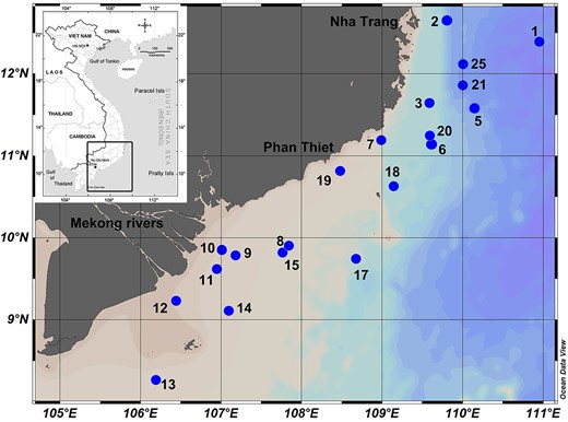
Maps showing Viet Nam with sampling area (rectangular, small map) and stations off the Vietnamese coast (largemap).
The information of sampling stations. OSW = offshore waters; UpW = upwelling waters; OnSW = nearshore waters; MKW = Mekong waters
| Station | Latitude | Longitude | B. Depth (m) | Sampling time | Water types |
|---|---|---|---|---|---|
| 1 | 12.3929 | 110.9509 | ~2000 | Day | OSW |
| 2 | 12.6512 | 109.8007 | ~570 | Day | UpW |
| 3 | 11.7142 | 109.5871 | ~130 | Day & night | UpW |
| 5 | 11.5802 | 110.1454 | ~1000 | Day | OSW |
| 6 | 11.1403 | 109.6174 | ~150 | Day | OSW |
| 7 | 11.1914 | 108.9879 | ~70 | Day | UpW |
| 8 | 09.8203 | 107.7627 | ~30 | Day | OnSW |
| 9 | 09.7854 | 107.1798 | ~25 | Night | MKW |
| 10 | 09.8531 | 107.0090 | ~25 | Day | MKW |
| 11 | 09.6252 | 106.9388 | ~25 | Day | MKW |
| 12 | 09.2327 | 106.4430 | ~25 | Night | OnSW |
| 13 | 08.2647 | 106.1927 | ~25 | Day | OnSW |
| 14 | 09.1108 | 107.0938 | ~30 | Day | OnSW |
| 15 | 09.7379 | 107.7626 | 35 | Day | OnSW |
| 17 | 09.7426 | 108.6736 | 90 | Day | OSW |
| 18 | 10.6278 | 109.1425 | 120 | Day | OSW |
| 19 | 10.8124 | 108.4674 | 28 | Night | UpW |
| 20 | 11.1377 | 109.6078 | 180 | Night | OSW |
| 21 | 11.8622 | 110.0011 | 1800 | Day | OSW |
| 25 | 12.1187 | 110.0028 | ~1900 | Day | OnSW |
The stations were grouped into four habitats based on a principal component analysis (PCA) using data of sea surface temperature (SST), sea surface salinity (SSS), mixed layer depth (DML), depth of chlorophyll maximum (zChlM) and nutrient availability index (NAI) of the upper 100 m of the water column (Weber et al., 2019). The NAI was designed to capture the impact of nutrient availability on phytoplankton (Weber et al., 2019; Nguyen-Ngoc et al., 2021). This index was defined by nitrate and nitrite concentrations and the depth where they reached 2 μM.
Sampling method
Zooplankton samples and measurements of environmental parameters were taken during the day at fifteen stations and during the night at four stations (Table I). At one station (station 3), samples were collected both during the day and the night to assess diel vertical migration.
Quantitative and qualitative samples were taken in vertical tows at speed of 0.5 ms−1 using a Juday net (37 cm diameter; 200-μm mesh size) with a release mechanism. Samples were collected at four depth intervals: 100–50 m, 50–25 m, 25–10 m and 10–0 m. The samples were fixed with formaldehyde (5% final concentration) and brought to the lab for later analysis.
Environmental parameters were measured using a CTD-rosette system (SBE 9+, Sea-Bird Electronics Inc., US) equipped with temperature, salinity and chlorophyll sensors.
Sample analysis
In the laboratory, samples were washed with freshwater to remove non-zooplankton items (e.g. microplastics, organic/inorganic fragments). The samples were then separated into large (>500 μm) and small (<500 μm) size fractions using a 500-μm sieve. The zooplankton size fractions were used to identify and count to species level under a stereomicroscopy (40—160× magnification) or a compound microscopy (Olympus BX53, Japan). Zooplankton in the large size fractions were all counted; the small size fractions were diluted (to a density of ca. 250–500 inds. mL−1) and 1-mL subsamples were counted. Zooplankton species were identified based on the literature (Chen, 1965; Chen, 1974), Owre (1967), Nishida (1985), Khoi (1994); Boltovskoy (1999) and Mulyadi (2002); (Mulyadi, 2004). Taxonomic information was updated based on Walter and Boxshall (2020).
Trait analysis
Copepod species were divided into three main trophic groups: carnivores, herbivores and omnivores (Troedsson et al., 2009; Lombard et al., 2011; Sullivan and Kremer, 2011; Navarro-Barranco et al., 2013; Tavares et al., 2013). We further divided the omnivorous copepods into smaller groups reflecting their general feeding tendencies (i.e. Omnivore–carnivore, Omnivore–detritivore and Omnivore–herbivore) as described by Benedetti et al. (2016).
Determination of the feeding, reproduction and diel migration of copepods were based on previously published studies (Kiørboe and Sabatini, 1994; Anjusha, 2013; Benedetti et al., 2016) and marine copepod databases (Razouls et al., 2020; Walter and Boxshall, 2020).
Copepods were assigned to one of four feeding types: ambush, cruise, current and mixed (Kiørboe and Sabatini, 1994; Kiørboe, 2011; Benedetti et al., 2016). The mixed feeders included taxa that showed both feeding-current and ambush feeders (Brun et al., 2017). The copepods in this study were clustered into two reproductive groups based on their egg-spawning strategy: broadcast-spawners and sac-spawners (Benedetti et al., 2016). Large number of copepod species were not be able to assigned to any reproductive group, classified as not applicable (N/A). This N/A reproductive group included species with no information or uncertain status (Supplementary Table 1).
Data calculation and statistical analysis
Statistical comparisons of the differences among the traits in different habitats and of the correlations among them and environmental parameters were carried out in SPSS (Ver. 17.0). Copepod abundance data (n = 82) in all habitats (n = 4) and depth stratum (n = 4) against environmental parameters (temperature, salinity and chlorophyll-a concentration) were used for non-parametric Spearman correlations. GraphPad Prism (Ver.6.0) was used to produce abundant figures of all traits.
We used copepod data (fourth root transformed) of 139 species (Supplementary Table 1) together with traits data of four functional traits (trophic group, feeding type, spawning strategy and maximal size) to perform a multiple correspondence analysis (MCA), following Benedetti et al. (2016; 2018) to delineate FG. The functional traits were transformed into numeric data for MCA analysis (Benedetti et al., 2018, 2018). Trophic groups were transformed into trinary data, 1, 2 and 3, corresponding to carnivore, non-carnivore and N/A, respectively. The non-carnivores included various categories of herbivores and omnivores (Supplementary Table 1). Similarly, feeding types and spawning strategies were also transform into trinary data, 1, 2 and 3. In feeding types, they were current feeding, other feeding groups and N/A group. In spawning strategies, they were broadcasters, sac-spawners and N/A group. The maximal body length was transformed into four size classes (SC1: 0.4–1.2 mm; SC2: 1.21–1.8 mm; SC3: 1.81–3.0 mm; SC4: 3.01–8.2 mm). Hierarchical clustering was performed on the MCA-derived distance matrix using Ward’s method (Legendre and Legendre, 2012). For identifying possible responses of copepods among the functional traits, habitats and depth strata, principle component analysis was performed. Analysis was performed using JMP software (SAS Institute Inc.).
RESULTS
Trophic groups
Trophic groups by habitats
Copepod trophic groups were unevenly distributed among the four habitat types. The most common trophic group was omni-herbivores (OH), followed by herbivores (H) and omni-detritivores (OD) (Fig. 2). The OH density was highest in the OSW habitat with 6.2 thousands inds. m−3 and also had the highest percentage (54%) in all habitats. The NA copepod group, including species were not assigned to any trophic group, contributed to an average of 12% of the total population density.
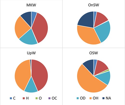
Variation of copepod trophic groups (abundant percentage) in different habitats, UpW, OnSW, MKW and OSW. C: carnivores, H: herbivores; O: omnivores; OC: omni-carnivores; OD: omni-detritivores; OH: omni-herbivores; NA: not applicable.
Some general trends were noticeable among the different habitats, including an increasing percentage of herbivorous (H) copepods from waters affected by the Mekong (MKW) to the waters affected by upwelling (UpW) and to offshore (OSW) areas, with the opposite trend in omni-herbivorous (OH) copepods. Three groups, carnivores (C), omnivores (O) and omni-carnivores (OC), were significantly lower than the other groups in all habitats (Fig. 2). The abundance of the carnivores (C) was relatively low in all areas and lowest in the UpW habitat. The OC trophic group was absent in the offshore stations (Fig. 2).
Among the habitats, the MKW and UpW were dominated by herbivorous (H) and omni-herbivorous (OH) copepods, which comprised 63 and 85%, respectively, of the total populations. In contrast, the OSW habitat was dominated by omni-herbivorous (OH group, 54%) copepods and the OnSW habitat was dominated by omnivorous copepods (OH and OD groups, in total 60%).
The vertical distribution of copepod trophic groups varied among habitats. At OSW and OnSW habitats, the density of all trophic groups decreased with depth, while it showed minor vertical variation in the MKW habitat and a mid-depth maximum in the UpW habitat. In the OnSW habitat, three dominant trophic groups: OH, OD and H were most abundance in the upper 25 m of water column. In the OSW habitat, this three dominant trophic groups (OH, OD and H) were also highest in the upper 50 m of water column.
Correlation of trophic groups and the environment
Our data showed a positive correlation between OD species abundance with chl-a concentration (P < 0.01, Spearman) in all habitats. The abundances of H and C species were positively correlated with temperature (P < 0.05), but negatively with salinity (P < 0.01 and P < 0.05, respectively, Spearman). In addition, abundance of D was negatively correlated with salinity (P < 0.05, Spearman).
Within habitats, we found a positive correlation between OD and chl-a concentration (P < 0.05, Spearman) in the UpW habitat and between H and temperature (P < 0.05, Spearman) in the OnSW habitat. Abundance of H in OnSW habitat was negatively correlated with salinity (P < 0.01, Spearman) (Supplementary Table 2).
Feeding types
Feeding type among habitats
Copepods were classified into four feeding types: ambush, cruise, current and mixed, with 16–33% being unclassified. Among the four habitats, current feeders were the most dominant group (42–57%), followed by ambush (8–15%) and cruise feeders (2–16%).
In the UpW habitat, the number of cruise feeders was 2-fold higher than the ambush feeders, which was opposite to the trend in the other three habitats. Proportions of cruise feeders (1.6–5.3%) and mixed feeders (0.2–0.3%) in the remaining three habitats (MKW, OnSW and OSW) were similar (Fig. 3).
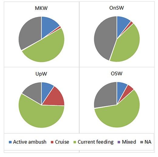
Distribution of copepod feeding types (percentage abundance) in different habitats, UpW, OnSW, MKW and OSW. NA: not applicable.
Vertical distributions of copepod feeding traits varied both within and among the habitats. Dominant groups were current feeders, and ambush feeders and they increased with depth in all three habitats, MKW, UpW and OnSW. These two feeding groups were dominance at surface in MKW, at upper 25 m of OnSW but at the 50–25-m layer of UpW habitats.
In the OSW habitat, the most dominant feeding group was the current feeders, which was high throughout the water column. Ambush feeders were similarly distributed to current feeders but at lower abundances.
Correlation between feeding traits and the environment
Among the feeding traits, ambush and cruise feeders showed a positive correlation with chl-a concentration (P < 0.01 and P < 0.05, respectively, Spearman). In the OnSW habitat, cruise feeders were positively correlated with chl-a concentration and the mixed feeders were negatively correlated with salinity (P < 0.05, Spearman). In the UpW habitat, both active ambush and cruise feeders were positively correlated with chl-a concentration (P < 0.05 and P < 0.01, respectively, Spearman) (Supplementary Table 2).
Reproductive behavior
Reproductive behavior by habitat type
In all habitat types, sac-spawners were more abundant than broadcast-spawners (Fig. 4), although 38–50% of the copepod populations could not be assigned to either of these categories. The densities of sac-spawners were six to seven times higher than broadcast-spawners in the MKW and UpW habitats. In contrast, sac-spawners were only four times more abundant than broadcast-spawners in the OnSW habitat and two times more abundant in the OSW habitat.
The two reproductive trait classes were low in abundance with a slight increase with depth in the MKW habitat. In the UpW habitat, sac-spawners reached a peak in abundance in the 50–25-m layer. In the OnSW habitat, the density of sac-spawners was highest from 25 to 10 m while the broadcast-spawners were rarer and decreased with depth. In the OSW habitat, both sac-spawners and broadcast-spawners were most abundant at the surface and decreased with depth.
Correlation between reproductive behavior and the environment
Among the reproductive groups, broadcast-spawning copepods showed a negative correlation with salinity, and sac-spawners showed a positive correlation with chl-a concentration (P < 0.05, Spearman). However, the correlation between sac-spawners and chl-a concentration was only significant at UpW habitat (r = 0.46, Spearman) (Supplementary Table 2).
Functional traits of copepod assemblages among habitats
There were seven copepod FG identified among habitats (Fig. 5). In the functional dendrogram (Fig. 5), the first separation was trophic groups. There were carnivores (FG1 and FG2), non-carnivores (FG 4–7) and N/A (FG3). In the second separation, spawning strategies were the main factor to define groups and minor separation were based on feeding and size. Among seven FGs identified, FG1 includes all carnivore, sac-spawning, active ambush and small to medium size copepods. All species of Ditrichocorycaeus were in this group. Other carnivorous, broadcasting and large size copepods were included in FG2. FG4 included omni-detritivorous, sac-spawning small size copepod with cruise and ambush feeders. The last three FGs (FG 5–7) include mostly broadcasting and current feeding copepods. FG5 included omni-herbivore and omnivore, large size species while GF7 included mostly herbivore and omni-herbivore, small-medium size species. FG6 included medium-large size species with mixed feeding types. The FG3 includes species were mostly not assigned to any traits.
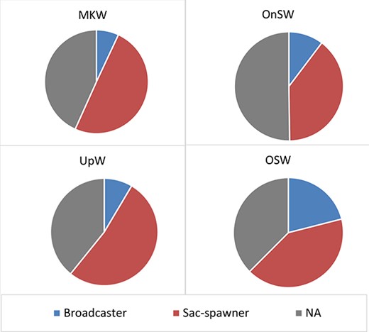
Distribution of reproductive traits (abundance percentage) of copepod in different habitats, UpW, OnSW, MKW andOSW.
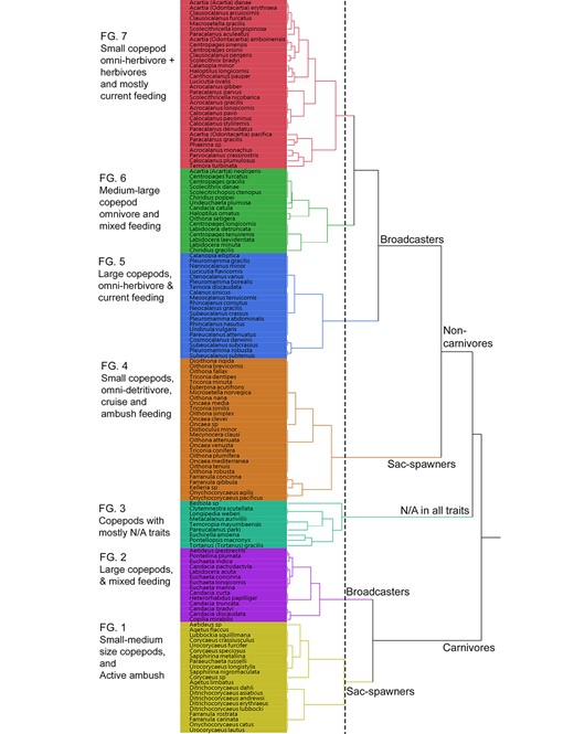
Functional dendrogram, obtained from an MCA and hierarchical clustering using Ward method, showing seven FG of the 139 analyzed copepod species. Dash line denotes where the tree was cut to form seven clusters.
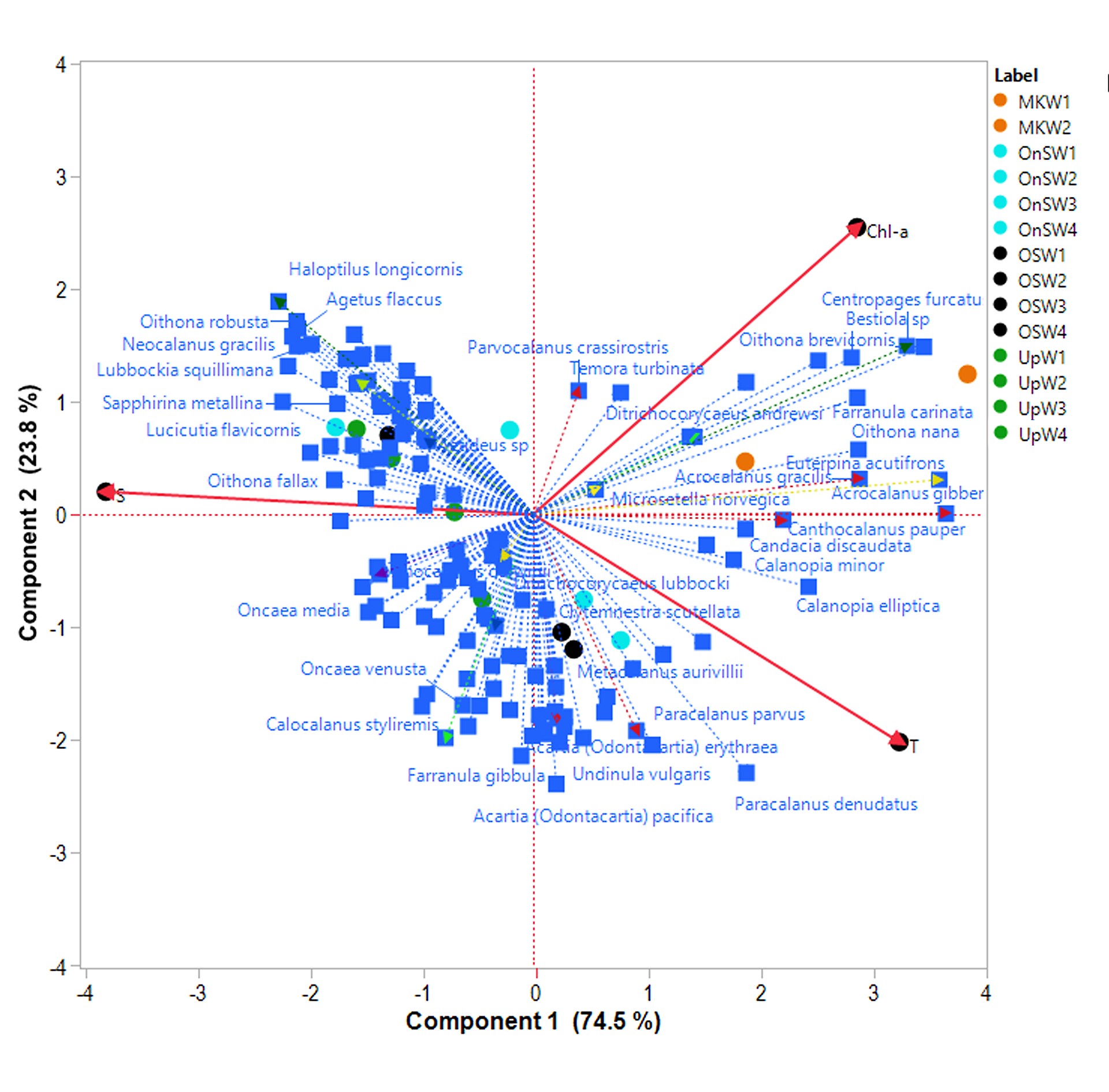
Principle component analysis all functional traits, habitats and depth strata revealed possible connection among the habitats and key species in different groups (Fig. 6). The first three PCs occupied 69.44% of variance. The first two PCs (PC1 = 49.5%; PC2 = 11.8%) separated upwelling communities from the other three habitats (OnSW, OSW and MKW). The first PC may be linked to salinity as it separated MKW to OnSW and OSW. The second PC was linked to temperature, with UpW and OSW4 in one group and MKW and OnSW in another. Nineteen most dominant species (Fig. 6), occupied 23.2–54.0% of copepod abundance in all habitats and depth strata. They belonged to six different FG. Each species or group species were associated with different habitats and/or depth strata. In the upwelling waters (UpW) and deeper water of OSW (OSW3,4), species of FG8 (Microsetella norvegica, Oithona plumifera) were likely important. The herbivores and herbivore-omnivores of FG7 were most associated in UpW (Calocalanus plumulosus, Parvocalanus crassirostris and Paracalanus parvus) and OSW (P. parvus). This FG7 included species that associate with higher Chl-a and/or higher temperature as further revealed by analysis with environmental variables (Fig. S1). Carnivores of FG 1 were scattered in deep stratum of OnSW (OnSW4, Urocorycaeus furcifer) and Mekong waters (MKW2, Ditrichocorycaeus andrewsi). The large carnivorous copepod Copilia mirabilis was associated with UpW (No 41, Fig. 6).
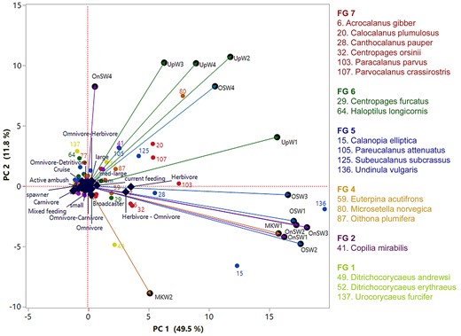
Principal component analysis (PCA) based on distribution and abundance data of 139 copepod species in four habitats and four depth strata and all trait categories. The abbreviations of the habitats are UpW, OnSW, MKW and OSW; depth strata 1 (0–10 m), 2 (20–25 m), 3 (25–50 m) and 4 (50–100 m). Species number, color and FGs were the same as in Fig. 5.
Diel vertical distribution
Diel vertical distribution of juvenile copepods
Three out of four juvenile copepods showed a short distance pattern of vertical migration. Paracalanus vertical distribution exhibited a shift toward the surface at night (Fig. 7) but WDM was small (Table II). Juveniles of Corycaeus showed a similar pattern, but with very different overall abundances between the day- and night-time samples. Juveniles of Corycaeus migrated long distance (dz = 25.6, Table II), between layers 10–0 m and 50–25 m. The juvenile of two genera, Oncaea and Oithona seemed to have short distance DVM (Table II). Oithona juveniles were at deeper layers, between 25 and 100 m, while Oncaea juveniles were shallower layers, between 0 and 50 m (Fig. 7).
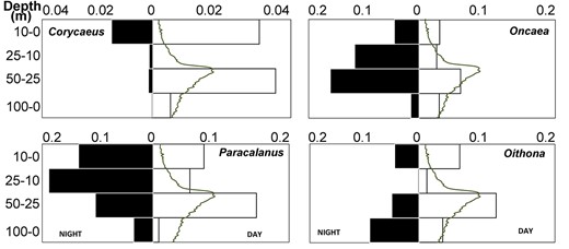
Diel changes in vertical distribution of four copepodite genera at station 3. Lines are chlorophyll-a concentration.
WDM during day and night and amplitude of the migration (dz) of selected taxa at station 3
| Genus/species | WDM (m) | dz (m) | |
|---|---|---|---|
| Day | Night | ||
| Corycaeus (Juvenile) | 37.6 | 11.9 | 25.6 |
| Oithona (Juvenile) | 45.3 | 62.4 | −17.1 |
| Oncaea (Juvenile) | 47.3 | 33.2 | 14.1 |
| Paracalanus (Juvenile) | 33.0 | 31.8 | 1.2 |
| Oithona nana | 21.8 | 26.4 | −4.5 |
| Oithona plumifera | 45.3 | 57.6 | −12.4 |
| Oncaea media | 41.5 | 44.7 | −3.2 |
| Oncaea mediterranea | 70.8 | 46.8 | 24.0 |
| Paracalanus parvus | 19.8 | 50.1 | −30.3 |
| Parvocalanus crassirostris | 7.7 | 25.8 | −18.0 |
| Triconia conifera | 35.7 | 50.4 | −14.7 |
| Triconia minuta | 63.8 | 49.6 | 14.1 |
Diel vertical distribution of adult copepods
Eight adult copepod species were chosen for DVM analysis, previously identified as strong (2 species), weak (4 species) and no (2 species) diel vertical migrators (Benedetti et al., 2016). At the station 3, a subsurface chlorophyll-a maximum of 0.86 μg·L−1 occurred at 51 m (Fig. 8). Six of the eight species showed DVM but in different degree (Table II). Oncaea media and Oithona nana did not show migration. Nocturnal upward migration was recorded in O. plumifera, P. parvus, P. crassirostris and Triconia conifera, with dz varied from −14.7 to −30.3 m (Table II). Reversed DVM was recorded in Oncaea mediterranea and Triconia minuta with dz = 24 and 14 m, respectively.
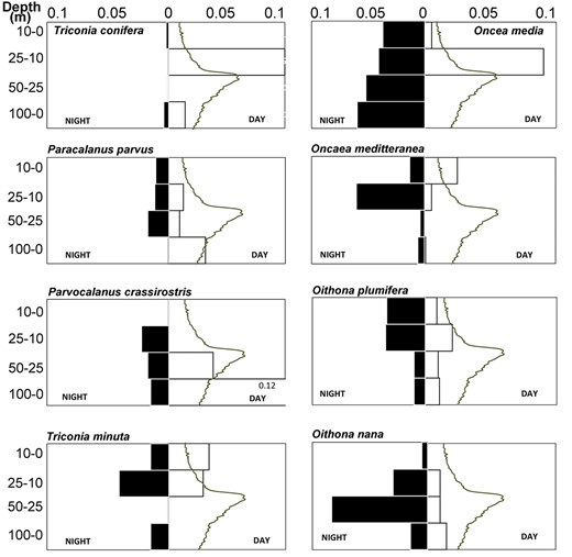
Diel vertical distribution of some mature copepods. Lines are chlorophyll-a concentration.
DISCUSSION
The biodiversity, biogeography and composition of zooplankton have been investigated in different coastal regions of Viet Nam (Nguyen and Truong, 2008; Truong et al., 2014; Truong and Nguyen, 2015a, 2015b). Prior studies have focused on the ecological and/or biological processes and interactions in plankton communities, especially in regions influenced by both the Mekong river outflow and coastal upwelling (Loick et al., 2007; Nguyen and Truong, 2008). However, this paper is the first to focus on characterizing zooplankton functional traits in the waters of Viet Nam. In the study region with various habitats, we found 7 FG of 139 copepods that were similar to previous studies in the Mediterranean Sea (Benedetti et al., 2016; 2018). The UpW and MKW areas were with dominance of herbivorous copepods while the other two habitats (OnSW and OSW) with dominance of omnivorous copepods. Our primary findings on DVM patterns of selected eight species were slightly different from previous reports, suggesting further investigation are needed for the region.
Zooplankton trophic groups
Copepod trophic groups (herbivores, omnivores or carnivores) provide critical insight into the ecological relationships between predators and prey (Chen et al., 2018). We defined trophic groups based on previous investigations on maxilliped structures and gut compositions of copepods (Wickstead, 1962). In addition to the three major trophic groups, we subdivided the omnivorous copepods based on feeding tendency, to produce a total of six trophic groups in all. The abundance of copepods that we could not assign to a trophic group varied among habitats, ranging from 1.3 to 22% of the total abundance.
Most copepods were omnivorous, with frequent occurrences of herbivorous, carnivorous or detritivorous feeding types as well (Turner, 2004; Calbet, 2008; Campos et al., 2017). We found that herbivores were more abundant than carnivores. We also found an increase in the relative abundance of herbivorous copepods from river (MKW) and upwelling (UpW) to offshore (OSW) waters. This is possibly related to the higher nutrient availability in waters influenced by the Mekong river and coastal upwelling, which could support higher rates of primary production and larger phytoplankton cells. The abundance of omni-herbivorous copepods increased from 25% in the river-influenced habitat (MKW) to 54% in the offshore (OSW) habitats. This group feeds on a broader food spectrum (suspended matters and phytoplankton) than herbivorous copepods, and seems to be more adapted to the OSW habitat. Other studies, have also found that omnivorous copepods were more abundant in oligotrophic waters in the Mediterranean Sea (Nowaczyk et al., 2011) or shifted from OH to OC in the western Tasman Sea (Henschke et al., 2015) which could be linked to food availability (Legendre and Rassoulzadegan, 1995). In our PCA results (Fig. 6) species associated with FG.7 were scattered in UpW1,2 (species 20, 107) and MKW1 (species 6, 32 and 28). Many previous studies have found that herbivorous copepods also prevailed near the thermocline and in waters with high chlorophyll concentrations (Longhurst, 1985; Williamson et al., 1996) with very small diurnal displacement (Dessier and Renédonguy, 1985). Similar patterns were found in the present study, especially in OnSW and OSW habitats (herbivore-omnivore, species 136, Fig. 6). Our results showed that omni-detritivorous copepods were positively correlated to chl-a concentration in all habitats.
The carnivore copepods FG1 and FG2 formed separated groups as in the Mediterranean Sea (Benedetti et al., 2018). However, FG1 in our waters was included with other small size copepods and it formed a group of small to medium size (Fig. 5) rather than large copepods in the Mediterranean Sea. The FG2 does contain genus Candacia as in the Mediterranean Sea (Benedetti et al., 2018), but with many other large size copepods. As such, this FG2 in our study was assigned to a larger carnivore group (Fig. 5).
Copepod feeding types
Our results showed that the most dominant feeding copepods were current feeders, followed by ambush and cruise feeders. The distribution of feeding types may depend on many factors such as body-size and temperature/season (Horne et al., 2016) or depth preference and season (Kenitz et al., 2017). Our study was carried out in the summer and revealed that ambush feeders were more abundant in the 25–10 m depth stratum in the MKW and OnSW habitats and in the 50–25 m stratum in the UpW area. Our PCA results also indicated FG 4 with many small ambush feeding copepod was associated closely to deeper strata of UpW as well as OSW4 (species 80, 87, Fig. 6). This is consistent with the findings of Kenitz et al. (2017), who reported that ambush feeders were distributed to a maximum 50 m in summer due to blooms of motileprey.
Zooplankton may employ different feeding behaviors in response to changing environmental conditions and prey abundance (Mariani et al., 2013). Forsbergh and Joseph (1964) reported that zooplankton biomass was higher in relation to the increase in chlorophyll concentration. We found that the abundances of ambush and cruise feeders were positively correlated to chl-a concentrations. According to Kiørboe (2017), the feeding behavior of copepods could be modified depending on the density of both prey and predators. We did not examine the prey–predator interaction in detail, but tested possible correlation among different functional copepod groups and those copepod groups to chlorophyll-a concentrations (as one type of food sources). In the four habitats, the cruising feeders were more abundant in OSW and OnSW, which may be related to the abundance of prey in these habitats. Lower chlorophyll-a concentrations were recorded, but other factors such as space (deeper water) or abundance of other food sources (e.g. carnivorous, omni-detritivorous and omni-herbivorous copepods) may contribute to their abundance.
Previous research has revealed some interrelationship among copepod traits. For example, correlated between feeding types and reproductive traits, cruise and ambush feeders are generally sac-spawners while current feeding copepods are broadcasters (Benedetti et al., 2016; Campos et al., 2017). We found similar correlation that the ambush and cruise feeding copepods and current feeding copepods are strongly correlated in all habitats with sac-spawning and broadcast spawning traits, respectively. However, there were some variation in these correlations. The correlation between current feeding and broadcasting groups was strongest in OSW, while the correlations between cruise and ambush feeding groups and sac-spawning group are strongest in UpW habitat.
Reproductive traits
We found that sac-spawners dominated over the broadcasters in all habitats with the density ratio between sac-spawners and broadcasters being higher in MKW and UpW habitats (7 and 6, respectively) than in OnSW and OSW habitats (4 and 2, respectively). Given advantages in fecundity of sac-spawners such as longer egg hatch times (Hirst and Bunker, 2003), much lower vulnerability and mortality and significant correlation to food limitations and higher temperature (Bunker and Hirst, 2004), the sac-spawners should have more advantages in MKW and UpW habitats than the broadcasters. Both of these habitats had more food sources (e.g. higher chl-a concentrations, 1.74 and 0.32 μg·L−1, MKW and UpW vs 0.27 and 0.26 μg·L−1, OnSW and OSW, respectively) and lower temperature in UpW habitat (Weber et al., 2019).
Growth and reproduction functional traits may be defined by various trait types including body size and reproduction (Litchman et al., 2013). Among those specific traits, one may have direct or indirect interactions with another or several other types. For example, studies on reproductive traits showed that sac-spawners were related to the mobility of organisms (e.g. males and females must meet for breeding) and this seems reasonable to the high motility species, which basically are carnivores (Benedetti et al., 2016). In our four habitats, the sac-spawners were correlated to other trait types, such as ambush feeders (r = 0.96, P < 0.0001, Spearman), omni-detritivorous (r = 0.99, P < 0.0001, Spearman) and omni-herbivorous feeders (r = 0.93, P < 0.0001, Spearman). Among our FGs 7, all sac-spawning copepods were in carnivorous group FG1 and omnivorous group FG4. These two groups are mainly active ambush feeders, especially FG1. Correlations between sac-spawners and carnivores were high but still lower than other trait types. We also found broadcasters in all the four habitats correlated with current feeders (r = 0.94, P < 0.0001, Spearman) with high tendency to omnivorous feeders including omni-detritivorous (r = 0.96, P < 0.0001, Spearman) and omni-herbivorous feeders (r = 0.95, P < 0.0001, Spearman). Benedetti et al. (2016) suggested that broadcasters are mainly current-feeders or mixed-feeders related to their shorter lifespans. The current feeding copepods were all broadcasters and grouped in either FG5 or FG7 for large and small body size, respectively (Fig. 5). These groups are more closely related to upwelling waters and surface waters of the Mekong (Fig. 6). The FGs 5 and 7 in the present study are similar to FGs 3 and 7 in the Mediterranean Sea (Benedetti et al., 2018) but with more species, 20 and 32 species, respectively.
Diel vertical migration
Four juvenile genera were chosen, Paracalanus, Oithona, Oncaea and Corycaeus, for DVM analysis due to their high abundances and showed remarkable DVM of different degrees. Study by Longhurst (1985) showed that at juvenile stages C1 to C4, Eucalanus inermis remains mainly in the upper 100 m around the chl-a maximum layers (C1 and C2) with short DVM. We found that three out of four genera also showed DVM with higher density around the chl-a maximum (25–50 m). Paracalanus juveniles did not having a clear DVM with a small dz but also was distributed around chl-a maximum. Studies in the Irish Sea revealed short (10 m) DVM amplitude of copepod nauplii at a coastal but longer DMV (20 m) at an oceanic station (Irigoien et al., 2004). In shallower coastal waters (20–30 m depth) in Hong Kong (Tang et al., 1994), Japan and Brazil (Checkley Jr. et al., 1992), there were no indication of DVM of adult Paracalanus (Hong Kong) or weak DVM of late juvenile (≥C4) of Paracalanus, Oithona, Oncaea and Corycaeus (Inland Sea of Japan). However, in the shallow and near coastal waters, advection transport of zooplankton may impact on diurnal migration. In the present study, juveniles of genus Oithona showed reverse DVM while the remaining three genera showed typical DVM. A previous study in the Irish Sea has revealed both reverse and typical DVM of C5 juvenile of P. parvus at both coastal and oceanic stations depending different sampling times (Irigoien et al., 2004). Juvenile C1-C3 of other genera Acartia and Calanus also have the same pattern (Irigoien et al., 2004).
Eight adult copepod species were selected based previous indication of strong (O. media and Triconia conifera), weak (O. nana, O. plumifera, O. mediterranea and Triconia minuta), and no DVM (P. parvus and P. crassirostris). One of the two strong DVM species (O. media) distributed around 60m with a reversed DVM, moving above the chlorophyll-max during the day and down during the night (Fig. 8). However, Triconia conifera seem to be transported elsewhere during the night. Previous studies on migration of Oncaeidae showed the greatest abundance of these species during both day and night during early summer period was in the upper 50 m in the upwelling north of Taiwan (Lo et al., 2004) and until late summer at ca. 50–100 m at the Kuroshio Extension region (Itoh et al., 2014). O. mediterranea showed the same pattern, with short amplitude nocturnal DVM in surface waters as in the Kuroshio Extension region (Itoh et al., 2014). However, this species was distributed deeper with longer amplitude during late summer. Triconia minuta has the same migration pattern with O. mediterranea in our study waters. In the Kuroshio Extension region, this species migrated within much deeper layers (ca. 50–150 m) with both reversed (during summer) and nocturnal (during winter) migration (Itoh et al., 2014). In our study, both Oithona species presented nocturnal migration but at different depth intervals, O. nana between 100 and 50 m and O. plumifera between 25 and 0 m. Studies in Irish sea revealed all Oithona species migrated over short distances nocturnally and reversed direction within upper 100 m of the water column (Irigoien et al., 2004). In upwelling station at North Taiwan Oithona atlantica did not showed a DVM (Lo et al., 2004) but the vertical distribution during 24 h suggested advection transport played important role on the species accumulation. Takahashi and Uchiyama (2008) had suggested that since Oithona species are all egg-carrying, they do not do DVM for reproduction but may do so for breeding and/or depth preference. In our study waters, observations on DVM were somewhat different (but not entirely opposite) to previous DVM pattern of the observed species, suggesting it is necessary to include more studies to fully understanding DVM patterns of copepods.
P. parvus showed a short reversed DVM between 25–50 and 50–100 m. In the Irish Sea, this species had nocturnal DVM during winter but reversed DVM during summer with variable amplitude around the year (Irigoien et al., 2004). The DVM pattern of the species in Viet Nam is similar to previous findings in Brazil (Gomes et al., 2004) that showed the migration was greater in deeper waters. P. crassirostris has similar DVM pattern as P. parvus. Both species are similar in size (0.69 ± 0.05 and 0.73 ± 0.04 mm of total length, respectively) and performed long nocturnal DVM (ca. 60 and 40, respectively). In shallow and eutrophic waters in Japan, P. crassirostris did not perform DVM (Checkley Jr. et al., 1992).
In the present study, most of genera/species performed nocturnal DVM as previous reported in adjacent waters (Lo et al., 2004; Itoh et al., 2014). For many copepod species, DVM is mainly driven by predator–prey interactions and thus depend on light varying in a day and vertically (Pinti et al., 2019). Our work showed the same pattern of DVM—that all species do migrate around the chlorophyll-a maximal layer and that food source was major reason that copepod species migrate.
The results of the present study confirm our prediction that impacts of Mekong River and coastal upwelling distinguish zooplankton assemblages with specific functional traits. Our analyses were confounded by the lack of information on a number of species. Most of species with unspecified traits were present in low abundance. However, our results were in consistent with previous studies and provide valuable contributions on functional trait characteristics of copepods, especially in tropical waters. Information on the biological characters of many copepod species used to identify traits is still needed to improve our understanding of functional trait characteristics in various ecosystems.
CONCLUSIONS
In the present study, as a first attempt to characterized functional traits of zooplankton in Viet Nam, we analyzed fourteen trait categories of four key functional traits (trophic, feeding, reproductive and diel migration) of copepods to investigate how environmental gradients impact on their distribution and abundance among the four defined habitats: MKW, UpW, OnSW and OSW. The results suggest that impacts of Mekong River and coastal upwelling led to distinct copepod assemblages with specific functional traits. Herbivorous species dominated in MKW and UpW, whereas omnivorous species dominated in OnSW and OSW. Sac-spawners dominated in all habitats, but decreased from MKW and UpW to OnSW and were lowest in OSW. Cruise feeders were 2-fold higher than ambush feeders in the UpW, but the opposite trend was found in the other habitats. There were seven functional groups of copepods identified in all four habitats, which similar to previous study in the Mediterranean Sea. These are valuable additions to copepod ecology, especially in tropical regions. However, it is necessary to conduct surveys in both dry and wet seasons to fully assess seasonal variations of feeding copepod traits.
Diel vertical distributions of copepods was used for DVM analysis. The observations on DVM were somewhat different from previously observed DVM patterns. The results were restricted in space and time, but provide guidance for future studies.
Our results provide contributions to our understanding of functional traits of copepod, and it is suggested that biological characteristics of many copepod species are needed to improve our understanding of functional trait in various ecosystems.
CONFLICT OF INTEREST
We have no conflicts of interest.
ACKNOWLEDGEMENT
The two anonymous reviewers are thanked for their valuable constructive suggestions. This paper is a contribution to celebrate the 100 years anniversary of the Institute of Oceanography, Viet Nam Academy of Science and Technology. We thank Prof. Kam Tang at Swansea University, UK and Prof. Walker Smith at Virginia Institute of Marine Science, USA, for critical comments and English corrections on the manuscript.
FUNDING
The National Foundation for Science and Technology Development (NAFOSTED) grant no. DFG 106-NN.06-2016.78. We thank the officers and crew of the R/V Falkor for their help and support at sea. The Schmidt Ocean Institute funded the sampling cruise FK060316.
References
Benedetti, F., Vogt, M., Righetti, D., Guilhaumon, F., and Ayata, S. D. (
