


Abstract
We recently proposed the equivalent width (EW) of the narrow [O iii]5007 Å emission line as an orientation indicator for active galactic nuclei. We tested this method on about 12 300 optically selected broad-line quasars from the SDSS seventh Data Release at redshift z < 0.8 and with full width at half-maximum values of broad emission lines (H α, H β, and Mg ii) larger than 2000 km s−1. We now examine their spectral energy distributions (SEDs) using broad-band photometry from the near-infrared to the ultraviolet to look for variations in the overall shape as a function of the EW[O iii]. We find that quasars with low EW[O iii] values (close to face-on position) have flatter near-infrared SEDs with respect to sources with high EW[O iii] values (almost edge-on). Moreover, quasars with high EW[O iii] values show a factor of ∼2 lower emission in the UV to quasars with low EW[O iii] values. Our findings indicate that the torus is clumpy and, on average, co-axial with the accretion disc and broad-line region, in agreement with the most recent theoretical models for the obscuring torus.
1 INTRODUCTION
We proposed the equivalent width (EW) of narrow [O iii] emission line as an orientation indicator for quasars (Risaliti, Salvati & Marconi 2011; Bisogni, Marconi & Risaliti 2017, hereafter Paper I). The anisotropy of the emission coming from the accretion disc (Shakura & Sunyaev 1973) and the properties of the [O iii] line at 5007 Å emitted by the Narrow Line Region (NLR) [isotropic and ascribable for the most part to active galactic nuclei (AGNs) activity] (Mulchaey et al. 1994; Heckman et al. 2004) allow us to use EW[O iii] as an indicator of source inclination with respect to the line of sight.
To test our method, we selected a large sample (|${\sim } 12\, 300$| objects) of unobscured type 1 quasars from the SDSS DR7 (Abazajian et al. 2009; Schneider et al. 2010), divided it in bins of EW[O iii] and created, for each one of them, a stacked spectrum meant to be representative of the bin (Paper I). All quasars have broad full width at half-maximum values larger than 2000 km s−1 of the most prominent broad emission lines (i.e. H α, H β, and Mg ii). The presence of orientation effects in both the broad and the narrow emission lines of optical/UV stacked spectra as a function of EW[O iii] has then proven the reliability of this quantity as an orientation indicator. Specifically, in the case of the lines emitted by the Broad-Line Region (BLR, e.g. H α, H β, and Mg ii) we recognized a broadening of the line profiles when moving from low EW[O iii] objects, corresponding to mostly face-on sources, to high EW[O iii] sources, corresponding to edge-on sources, in agreement with BLR models that describe the geometry of this structure as disc shaped (Pancoast et al. 2014; Grier et al. 2017). In the case of lines emitted by the NLR, represented by the [O iii] 5007 Å line itself, we observed a statistically significant decrease both in the shift of the central velocity with respect to the reference wavelength and in the intensity of the blue component of the line when moving from low to high EW[O iii], in agreement with the presence of gas in outflow in this region, that we are able to intercept preferentially when the source is face-on. The presence of such effects on spectroscopic features confirms that the orientation of the source with respect to the line of sight is one of the main drivers of the variance of quasars spectra, although not the only one (SMBH mass, Eddington ratio, etc., e.g. Marziani et al. 2003; Shen & Ho 2014).
We now investigate the quasar broad-band spectral energy distributions (SEDs) from the near-infrared to the ultraviolet to look for variations in the overall shape as a function of the EW[O iii]. Specifically, we focus on the near-infrared emission, which is usually ascribed to a dusty structure surrounding the disc at parsec scales (the so-called torus) proposed in the orientation empirical model (Antonucci 1993; Urry & Padovani 1995). This component, coplanar with the accretion disc but with much larger scale height (Krolik & Begelman 1988; Hicks et al. 2009) to hide the inner components, has been recently proposed to be characterized by a clumpy (e.g. Nenkova et al. 2008a, b; Nikutta, Elitzur & Lacy 2009; Hönig & Kishimoto 2010; Stalevski et al. 2012; Siebenmorgen, Heymann & Efstathiou 2015), rather than smooth (Pier & Krolik 1992; Fritz, Franceschini & Hatziminaoglou 2006) structure. The clumpy description fits well with the results of Paper I: given the selection we applied to our sample, only blue, type 1 objects are included; the fact that we can intercept the accretion disc and BLR emission even in edge-on positions is therefore a confirmation that – if present – the obscuring component cannot be at the same time smooth and coplanar with the inner components. Only three scenarios are then plausible: (1) an obscuring structure not present at all, (2) the torus is misaligned with respect to the accretion disc and the BLR, or (3) the torus is clumpy and we can have a line of sight of the inner regions even if they are coplanar. An analysis of the emission in the IR band of the same sample as a function of EW[O iii] is therefore required in order to have information on the properties of the torus. We analyse the SED of the sources in the sample using the UV/optical/IR photometry available in literature, then focusing on the part of the SED ascribable to the torus.
This paper is organized as follows: in Section 2 we describe the data; in Section 3 we discuss the analysis we performed interpolating the photometric data available. In Sections 4 and 5 our results and their implications on the properties of the torus are presented and discussed. In this work, the following cosmological parameters are assumed: H0 = 70 km s−1 Mpc−1, ΩM = 0.3, and ΩΛ = 0.7.
2 DATA
2.1 The sample
Our sample was selected from the Quasar Catalogue of the Sloan Digital Sky Survey (SDSS) DR7 (Schneider et al. 2010) – through the properties compiled in the catalogue by Shen et al. (2011) – to be first composed of objects whose [O iii] emission falls in the optimal response window of the SDSS spectrograph (0.001 < z < 0.8). We then selected quasars with an absolute magnitude Mi < −22.1 and a median signal to noise per pixel for the rest frame 4750–4950 Å region S/N ≥ 5. The final requirement was for the EW[O iii] to be in the range 1–300 Å (Risaliti et al. 2011), so to exclude sources with an incorrect measure of the [O iii] line. This selection yielded a sample of |${\sim } 12\, 300$| quasars.
2.2 Photometric data
We collected broad-band photometry from IR to the UV using data from all sky surveys, such as WISE, 2MASS, SDSS, and GALEX, to allow a proper determination of the emission coming from the accretion disc and the obscuring torus.
The Galaxy Evolution Explorer (GALEX) is an ultraviolet space telescope that performed a survey in the FUV (1350–1780 Å) and NUV (1770–2730 Å) ultraviolet bands. We used the GALEX photometric data from the sixth release (GR5) (Bianchi et al. 2011), listed in the ancillary columns of the Shen et al. (2011) catalogue. 87 per cent of our sample has a measurement in at least one of the two bands and the |$77{{\ \rm per\ cent}}$| has both the bands available.
The sample was originally selected from the fifth Quasar Catalogue SDSS DR7 (Schneider et al. 2010), therefore our sources have all the five optical SDSS magnitudes (ugriz, from 3000 to 9000 Å) available. We used the SDSS psfMag magnitudes listed in the catalogue of Shen et al. (2011), i.e. a magnitude obtained fitting a Point Spread Function (PSF) model to the source, optimal for point sources.
In the near-infrared range, we collected data from the Two Micron Sky Survey (2MASS, Skrutskie et al. 2006) in the J (|$1.24 \, \mu$|m), H (|$1.66 \, \mu$|m), and K (|$2.16 \, \mu$|m) bands. We matched the sources in our sample to the All-Sky Point Source Catalogue and the Reject Table,1 requiring a maximum separation between the sources of 2 arcsec. When a source was not detected in the survey, we used the IDL routine aper to infer an upper limit for the magnitudes on the 2MASS images. Specifically, for each band, we downloaded the 2MASS image, we evaluated the magnitude in a region of radius 4 arcsec centred at the expected position of the source and we estimated the sky background in an annular region with inner radius 14 arcsec and outer radius 20 arcsec. We repeated the evaluation of the sky background randomly selecting 1000 circular regions at a distance smaller than 100 arcsec from the nominal position of the source. We considered a detection if the flux of the source was larger than the 95th percentile of the distribution of 1000 values for the sky background, otherwise we took the 95th percentile as a 2σ upper limit. We then applied – to both detections and upper limits – the aperture correction corresponding to the image on which the aperture photometry was performed, as listed in the Atlas Image Information Table.2
We finally considered the four IR photometric bands of Wide-field Infrared Survey Explorer (WISE, Wright et al. 2010): W1 (|$3.4 \, \mu$|m), W2 (|$4.6 \, \mu$|m), W3(|$12 \, \mu$|m), and W4(|$22 \, \mu$|m). We matched our sample to the WISE All-Sky Source Catalogue within a 2 arcsec matching radius and, where a match was not found, we searched the WISE All-Sky Reject Table.3 Ninety-nine per cent of the sample has three out of the four photometric bands available and only the |$13{{\ \rm per\ cent}}$| of the sample has the W4 band missing. We used the WISE profile-fitting magnitude, the optimal choice for point-like sources. The WISE All-Sky Source Catalogue already provides upper limits when the sources are not detected. In the whole sample we only have a few tens of sources for which a measure is not available at all.
All the photometric data are corrected for Galactic reddening, using the E(B − V) values as estimated from the Schlegel, Finkbeiner & Davis (1998) map, using an RV = 3.1 and the extinction law by Fitzpatrick (1999).
3 DATA ANALYSIS
To verify whether quasars SED have a trend with the EW[O iii], we stacked the photometric data similarly to what we did with the optical spectra in Paper I: (1) we divided the sample in six (equally spaced in log) EW[O iii] bins (Table 1); (2) within each bin, we rest-framed the data points accordingly to the improved measurements for the redshifts listed in the SDSS-DR7 catalogue (Hewett & Wild 2010); (3) we performed a linear interpolation of the photometric data points for each source; (4) we normalized the interpolated SED to the value corresponding to a reference wavelegth (|$\lambda _{\mathrm{ref}}=15 \, \, \mu$|m4) in the mid-IR, representative of the spectral range in which the torus emits. Differences in the IR emission can be ascribed to the intrinsic properties of the individual sources, both of the torus and of the primary source. Through this normalization, we can make a comparison between the sources that is unbiased by these intrinsic differences.5; (5) we stacked all the SED in a given EW[O iii] bin to obtain a ‘representative’ SED for a given inclination angle range. In order to do that, all the SED were interpolated on a common wavelength grid and, for each spectral channel, the median value was considered. Fig. 1 shows the rest-framed, photometric data (points) for all the sources in the sample, divided in the six EW[O iii] bins. The solid lines are, from top to bottom, the 84th, 50th (median), and 16th percentiles – in each spectral channel – of the distribution of the SED obtained by interpolating the photometric data points for each source and then normalizing to the flux corresponding to the reference wavelength of |$15 \, \mu$|m.
![Rest-framed photometric data points for each source in the sample (points) in six EW[O iii] intervals, normalized to the flux corresponding to the reference wavelength $\lambda =15 \, \mu$m. The solid lines are the 84th, 50th (median), and 16th percentiles – in each spectral channel – of the distribution of the SED obtained by interpolating the photometric data points for each source.](https://oup.silverchair-cdn.com/oup/backfile/Content_public/Journal/mnras/485/1/10.1093_mnras_stz495/1/m_stz495fig1.jpeg?Expires=1716968206&Signature=MWIDm1fciyTOk7bpAbgHXWDLzgXUUs8~0vDxl-iRpmNgyN7MkbsbZYu3Rohl9L4DvrUMRDlMBndjBIsxZsCrfK37kfAqEz9F~vxKxWqlT85Z2DVGiGQSqagwbRjeEc6D8FTUqMjKURbZmTdIyIWwKsHotu1wSOe4E0Ac2pRmlI-kmdrEaF81tw9iDYtJwVCrFYGW1Wd29FjAhG5QZU~MHW7-vAWEIxGpqTASVue86Gw2DBupeSbVuhmuTh9X1cWi0fgyXctyhz8OddWE8mwzrI~4aXImbK5lqdXEFDi1YqMvyixNUlnF6FZBM42rh3JYvGzKGzjDbZL4h4-qlAcO1w__&Key-Pair-Id=APKAIE5G5CRDK6RD3PGA)
Rest-framed photometric data points for each source in the sample (points) in six EW[O iii] intervals, normalized to the flux corresponding to the reference wavelength |$\lambda =15 \, \mu$|m. The solid lines are the 84th, 50th (median), and 16th percentiles – in each spectral channel – of the distribution of the SED obtained by interpolating the photometric data points for each source.
Bins of EW[O iii]. We divided the sample in equally spaced bins in log(EW[O iii]), the same as in Paper I. * The first two bins have been merged in a single one. For each bin, we list mean values and uncertanties assuming a Gaussian distribution and median and 16th and 84th percentiles (1σ interval) for log(MBH), log(L5100), log(Lbol) and for the Eddington ratio, based on the data from the catalogue of Shen et al. (2011).
| ΔEW | EW | n | log(MBH/M⊙) | log(L5100/ergs−1) | log(Lbol/ergs−1) | REdd | ||||
|---|---|---|---|---|---|---|---|---|---|---|
| [Å] | [Å] | Mean | Median | Mean | Median | Mean | Median | Mean | Median | |
| |$1\text{--}6 ^{\, *}$| | 3.0 | 1095 | 8.392 ± 0.017 | |$8.4^{+0.5}_{-0.5}$| | 44.606 ± 0.012 | |$44.5^{+0.4}_{-0.3}$| | 45.571 ± 0.012 | |$45.5^{+0.4}_{-0.3}$| | −0.921 ± 0.017 | |$-0.8^{+0.5}_{-0.7}$| |
| 6–12 | 9.0 | 3443 | 8.433 ± 0.008 | |$8.4^{+0.5}_{-0.5}$| | 44.601 ± 0.005 | |$44.6^{+0.4}_{-0.3}$| | 45.566 ± 0.006 | |$45.5^{+0.4}_{-0.3}$| | −0.967 ± 0.008 | |$-0.9^{+0.4}_{-0.5}$| |
| 12–25 | 18.5 | 4389 | 8.474 ± 0.007 | |$8.5^{+0.5}_{-0.5}$| | 44.587 ± 0.005 | |$44.6^{+0.4}_{-0.3}$| | 45.553 ± 0.005 | |$45.5^{+0.4}_{-0.3}$| | −1.021 ± 0.007 | |$-1.0^{+0.4}_{-0.5}$| |
| 25–50 | 38.5 | 2375 | 8.526 ± 0.010 | |$8.5^{+0.5}_{-0.5}$| | 44.561 ± 0.007 | |$44.5^{+0.4}_{-0.3}$| | 45.526 ± 0.007 | |$45.5^{+0.4}_{-0.3}$| | −1.101 ± 0.009 | |$-1.1^{+0.4}_{-0.5}$| |
| 50–100 | 75.0 | 810 | 8.520 ± 0.016 | |$8.5^{+0.5}_{-0.5}$| | 44.519 ± 0.012 | |$44.5^{+0.4}_{-0.3}$| | 45.483 ± 0.012 | |$45.5^{+0.4}_{-0.3}$| | −1.137 ± 0.015 | |$-1.1^{+0.4}_{-0.4}$| |
| 100–250 | 175.0 | 190 | 8.466 ± 0.039 | |$8.4^{+0.6}_{-0.5}$| | 44.470 ± 0.021 | |$44.4^{+0.4}_{-0.3}$| | 45.437 ± 0.021 | |$45.4^{+0.4}_{-0.3}$| | −1.129 ± 0.038 | |$-1.1^{+0.5}_{-0.6}$| |
4 RESULTS
![Comparison of the stacked SED obtained from the photometric data points for the six EW[O iii] bins. Moving to high EW[O iii], we see the IR part of the SED steepening, as expected in a clumpy torus scenario.](https://oup.silverchair-cdn.com/oup/backfile/Content_public/Journal/mnras/485/1/10.1093_mnras_stz495/1/m_stz495fig2.jpeg?Expires=1716968206&Signature=fMUeVk3je6Ao9vVXApGKaW~TxQDEk27bHNUUB02x0B~dMxxG6Q14jRTz4z4AeH0ou~6ihIdO6-0lr~5zM9Bu~4AC-2mP1UKnkt7EbZkRm5XDp80BD66nJbxTNyg38FIjlw6s9By2s4KcM8P1nMnad5y3Bg7WPu8qMv8GfbwtX0UPAATEFhP47InYhX0BrYyevy6zXeP8-gZT1DLljh3oVqrGv701RSpDPgFVEDwWDCc0S~UIAx9fhkljoci6GSYmGP4aIFDeWRJD6H4~JMrbPWfZQNiM4PNg4mMEw-6xfderKc-yU82gpayCwk58jPXwambtYdTvcVCdYRYDDXcICg__&Key-Pair-Id=APKAIE5G5CRDK6RD3PGA)
Comparison of the stacked SED obtained from the photometric data points for the six EW[O iii] bins. Moving to high EW[O iii], we see the IR part of the SED steepening, as expected in a clumpy torus scenario.
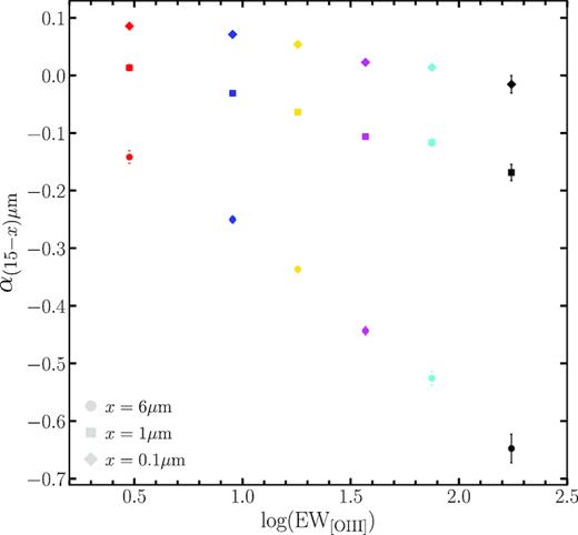
Energy slopes, as defined in equation (1), for the six stacked representative SED. The circles, squares, and diamonds indicate the slope (15–6) |$\mu$|m, (15–1) |$\mu$|m, and (15–0.1) |$\mu$|m, respectively.
Energy slopes, as defined in equation (1), for the six stacked representative SED.
| ΔEW | EW | |$\alpha _{(15-6)\, \mu \mathrm{m}}$| | |$\alpha _{(15-1)\, \mu \mathrm{m}}$| | |$\alpha _{(15-0.1)\, \mu \mathrm{m}}$| |
|---|---|---|---|---|
| [Å] | [Å] | |||
| |$1\text{--}6 ^{\, *}$| | 3.0 | |$-0.142_{-0.011}^{+0.010}$| | |$+0.013_{-0.006}^{+0.006}$| | |$+0.086_{-0.006}^{+0.004}$| |
| 6−12 | 9.0 | |$-0.250_{-0.006}^{+0.005}$| | |$-0.031_{-0.003}^{+0.003}$| | |$+0.071_{-0.002}^{+0.002}$| |
| 12−25 | 18.5 | |$-0.337_{-0.005}^{+0.005}$| | |$-0.063_{-0.003}^{+0.003}$| | |$+0.053_{-0.002}^{+0.002}$| |
| 25−50 | 38.5 | |$-0.443_{-0.007}^{+0.007}$| | |$-0.106_{-0.004}^{+0.004}$| | |$+0.023_{-0.003}^{+0.003}$| |
| 50−100 | 75.0 | |$-0.526_{-0.011}^{+0.012}$| | |$-0.117_{-0.007}^{+0.006}$| | |$+ 0.014_{-0.006}^{+0.004}$| |
| 100−250 | 175 | |$-0.65_{-0.02}^{+0.02}$| | |$-0.169_{-0.014}^{+0.015}$| | |$-0.015_{-0.015}^{+0.007}$| |
5 DISCUSSION
We have demonstrated that the EW[O iii] parameter computed from low/moderate-resolution spectra (i.e. 1500 at 3800 Å) can be used as a proxy for the inclination of the accretion disc in quasars. Of the three possible explanations for the detection of broad-line emission in quasars at high inclination angles (see Section 1), only one is plausible. This is due to two factors: (1) we observe a mid-IR emission and therefore the torus cannot be missing, (2) the decrease in the IR emission at shorter wavelengths as a function of EW[O iii] is progressive – as it is with the increase in the broad lines width in paper I; therefore a misaligned torus with respect to the inner components, i.e. BLR and accretion disc, is excluded. The only possibility is that we can intercept the emissions coming from the BLR despite the presence of the torus, i.e. the torus must be clumpy. In the following, we discuss how the behaviour of the SED as a function of EW[O iii] is exactly what is expected in a clumpy torus scenario.
The most recent models for the obscuring structure suggest that it is to be composed of clouds of molecular gas and dust (Nenkova et al. 2008a, b; Nikutta et al. 2009), in some cases permeated by a diffuse medium ‘filling’ the empty regions between the clouds (Hönig & Kishimoto 2010; Stalevski et al. 2012; Siebenmorgen et al. 2015; Hönig & Kishimoto 2017). As already mentioned, the clumpiness of the torus is a condition we need in order to explain the results of Paper I: we are able to intercept the emissions coming from the BLR even in sources close to the edge-on position, something that could not be explained with a smooth, optically thick torus. We want to examine the emission in the IR band as a function of EW[O iii] to see if it is in agreement with what is expected by the clumpy models. We considered the models by Nenkova et al. (2008a, b) and Nikutta et al. (2009), which depict the torus as a toroidal distribution of clouds, whose emission, result of the re-processing of the emission of the accretion disc, can be described with a set of parameters, among which the inclination with respect to the line of sight of the observer. The IR emission we can observe from a face-on torus is overall higher than the one coming from a torus in an edge-on position, due to the fact that in the first case we are looking at a larger portion of the emitting structure. However, as the intensity of the IR emission cannot be associated with the inclination of the accretion disc (it can be due to intrinsic differences in the properties of the individual source, such as the dimension and the covering factor of the obscuring structure, the ratio between its inner and outer radius, the properties of the emission coming from the primary source etc.), to define a reference wavelength in normalizing the SED in the various bins, we have chosen a near-IR wavelegnth (i.e. 15 |$\mu$|m). One of the most important assumption in our work is that the distribution of the tori in each bin is similar, i.e the physical properties of the torus, the dust distribution, the number of clouds, etc. are similar on average amongst the EW[O iii] bins. These models predict a drop in the IR emission at the shorter wavelengths (|$\lambda \sim 1 \, \mu$|m) with respect to the longer ones (|$\lambda \gt 5 \, \mu$|m) moving from low to high inclination angles. This result is due to the combination of two different effects: (1) going towards edge-on positions we are intercepting a higher number of clouds and (2) the absorption caused by the clouds is more efficient at the shorter with respect to the longer wavelengths. Regardless of the intrinsic distribution of the properties of the individual sources, moving from face-on to edge-on positions, the shape of the IR emission progressively steepens, with a stronger decrease in the ‘blueward’ with respect to the one in the ‘redward’ part. This effect can be seen in Fig. 4, where we show the shape of the torus SED as a function of the line of sight of the observer as obtained using the theoretical SED in the CLUMPY library7 (Nenkova et al. 2008a, b; Nikutta et al. 2009). This comprehensive data base contains more than 1 million of models for type 1 and type 2 AGN SED obtained varying a set of six parameters8 describing the physical and geometrical properties of the torus component, among which the inclination of the nucleus with respect to the line of sight. CLUMPY also provides derived properties, such as the probability of having an unobscured AGN based on the aperture angle of the torus, as measured from the equatorial plane of the nucleus, and the inclination angle. To create this set of templates we did not exclude type 2 AGN, as defined by this parameter, since in our interpretation we can have a type 1 AGN even with a high inclination, i.e. with i > 45°, as long as the line of sight is free by intervening clouds. The aim of this study is to examine the variation of the torus SED as a function of the inclination angle i. We then create these templates considering, in each spectral channel, the median value of the whole set of templates with a given inclination angle (see Fig. 4), so to allow a comparison of the SED for our data to the theoretical models. Moving from a small to a high inclination angle, we can see the decrease in the IR emission in the shorter wavelengths with respect to the longer ones.
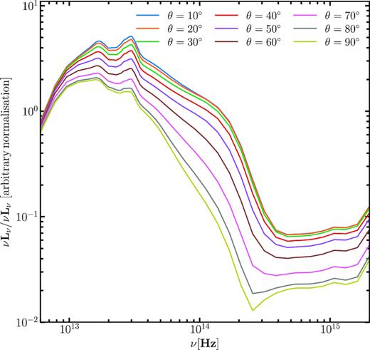
CLUMPY models as a function of the inclination angle of the torus with respect to the line of sight. The CLUMPY library contains more than 106 theoretical SED, obtained varying the set of parameters describing the physics and geometry of the torus.
This is exactly what we see in our data, once we compare the representative SED for the EW[O iii] bins (Fig. 2). Moreover, the gradual steepening of the mid-IR SED with increasing inclination angle, as opposed to the bimodal transition in the SED shape predicted by a sharp-edge geometry of the distribution of the clouds (Nenkova et al. 2008b), suggests that a Gaussian angular distribution of the clouds is more representative of the obscuring structure.
We tried to fit these models to the average SEDs, but the ones corresponding to low inclination angles are still too steep to provide a good representation of the quasar stacks. The torus models are missing an extra component that takes into account the emission produced by the hottest dust in the torus, the inner edge of the dust cloud distribution – and discussed in the most recent works on the IR SED in quasars and AGN (Mor, Netzer & Elitzur 2009; Deo et al. 2011; Mor & Netzer 2012; Duras et al. 2017; García-González et al. 2017; Hönig & Kishimoto 2017; Shangguan, Ho & Xie 2018). None the less, we clearly see the decrease in the shortest wavelengths emission of the IR SED moving from low to high EW[O iii] (see Table 2). Given that in each EW[O iii] the sources are similarly distributed in terms of BH mass, luminosity and Eddington ratio (Table 1), we cannot find any other physical explanation to this trend other than the effect produced by the orientation of the torus.
As already stressed in paper I, we do not claim the orientation to be the only driver in the variance of quasars spectra in general, or in the IR SED for the specific case of the torus. Other physical drivers may contribuite to make the physical properties and the geometry of the system – and therefore the SED – different. In the case of the torus, both primary source properties – such as the accretion rate (Ezhikode et al. 2017; Ricci et al. 2017) or the luminosity (Maiolino et al. 2007; Treister, Krolik & Dullemond 2008; Lusso et al. 2013), and composition of the torus clouds (Alonso-Herrero et al. 2011; Ramos Almeida et al. 2011; Audibert et al. 2017) can change the shape of the IR emission. We do note again, however, that, as for this study has been designed, the effects produced by drivers other than orientation are ‘blended’ within the EW[O iii] bins. The effect produced by the orientation is the only one recognizable in the stacking we performed.
We are undertaking a complete SED fitting to our data using AGN fitter (Calistro Rivera et al. 2016), a Bayesian MCMC code that takes into account four emitting components for reproducing the total emission of AGN: the accretion disc, responsible for the Big Blue Bump in the optical/UV, the hot dust torus, the stars in the host galaxy, and the cold dust in star-forming regions. As already mentioned, a preliminary analysis on our sample has revealed that, to properly treat the effect produced by the orientation on quasars SED, we need to include an extra blackbody component. This will be the subject of a forthcoming paper.
6 CONCLUSIONS
In this work we constructed the broad-band SED of |${\sim } 12\, 300$| SDSS DR7 quasars and analysed the overall shape as a function of the inclination angle of the accretion disc with respect to the line of sight. The EW[O iii] orientation indicator allows us to split the sample in bins of different inclination angles and examine the presence of orientation effects on the SED of quasars. In previous works on the EW[O iii] orientation indicator, we found that broad emission lines are detectable even in sources close to an edge-on position, in agreement with the most recent models depicting the torus as a clumpy rather than a smooth structure. In this sense, type 1 AGN are sources for which the line of sight is free from intervening clouds, regardless of their inclination.
We focus on the IR bands of the SED – related to the emission from the obscuring torus – looking for information on the properties of this structure in light of its inclination with respect to the observer. Our findings are the following:
We do see a clear trend of the representative SED we created dividing the sample in EW[O iii] bins. Our sample is composed of objects with every kind of luminosity, accretion rate, BH mass, and other properties of AGN components, and since it has been divided only in terms of EW[O iii], a quantity that is defined to be a function of the inclination of the accretion disc with respect to the line of sight, we interpret the behaviour of the representative SED as a confirmation of the reliability of this quantity as an orientation indicator.
We do detect an emission in the mid-IR wavelenght range, therefore the torus cannot be missing. To check that the IR bump is not produced by blazar-like objects, we performed the stacking analysis on the 8 per cent and 92 per cent of quasars that show strong radio emission and that are radio-quiet, respectively, and found the same results.
The IR SED gradually steepens moving from low EW[O iii] (face-on) to high EW[O iii] (edge-on) objects (Table 2 and Fig. 3). EW[O iii] is a strong function of the inclination of the geometrically thin accretion disc. Given that the energy slopes decrease so neatly with EW[O iii], it means that the obscuring structure on a statistical sense has then to be co-axial with accretion disc and BLR. Our results also imply that the torus has a clumpy structure. From the results of Paper I we know that we can intercept the broad emissions even in sources in a position close to the edge-on; the torus has therefore to be composed of clumps rather than of a smooth continuum of gas, and our ability of intercepting the broad lines is related to the probability of having a line of sight free by intervening clouds.
The decrease of the IR emission at the shorter with respect to the longer wavelengths is in agreement with what expected from the theoretical models for clumpy tori.
We conclude that the only possible explanation for type 1 objects in position close to the edge-on, i.e. for the detection of broad emission lines, is a torus with a clumpy structure. The use of EW[O iii] as an orientation indicator for quasars allows us to verify the presence of orientation effects on the IR SED. The orientation plays a major role in determining the shape of the SED in quasars, although it is not the only driver. Other physical drivers (e.g. SMBH mass, luminosity, Eddington ratio) may compete in shaping quasars emission. This work is however designed to isolate the effects produced by the orientation; in each inclination range we are averaging sources that span a wide range in terms of luminosity, accretion rate, and composition.
ACKNOWLEDGEMENTS
SB and GR acknowledge support from the grant ASI-INAF N. 2017-14-H.0. SB is supported by NASA through the Chandra award no. AR7-18013X issued by the ChandraX-ray Observatory Center, operated by the Smithsonian Astrophysical Observatory for and on behalf of NASA under contract NAS8-03060. SB was also partially supported by grant HST-AR-13240.009. EL is supported by an EU COFUND/Durham Junior Research Fellowship under grant agreement no. 609412. Funding for the SDSS and SDSS-II has been provided by the Alfred P. Sloan Foundation, the Participating Institutions, the National Science Foundation, the U.S. Department of Energy, the National Aeronautics and Space Administration, the Japanese Monbukagakusho, the Max Planck Society, and the Higher Education Funding Council for England. The SDSS Web Site is http://www.sdss.org/. The SDSS is managed by the Astrophysical Research Consortium for the Participating Institutions. The Participating Institutions are the American Museum of Natural History, Astrophysical Institute Potsdam, University of Basel, University of Cambridge, Case Western Reserve University, University of Chicago, Drexel University, Fermilab, the Institute for Advanced Study, the Japan Participation Group, Johns Hopkins University, the Joint Institute for Nuclear Astrophysics, the Kavli Institute for Particle Astrophysics and Cosmology, the Korean Scientist Group, the Chinese Academy of Sciences (LAMOST), Los Alamos National Laboratory, the Max-Planck-Institute for Astronomy (MPIA), the Max-Planck-Institute for Astrophysics (MPA), New Mexico State University, Ohio State University, University of Pittsburgh, University of Portsmouth, Princeton University, the United States Naval Observatory, and the University of Washington. This publication uses data products from the Two Micron All Sky Survey, which is a joint project of the University of Massachusetts and the Infrared Processing and Analysis Center/California Institute of Technology, funded by the National Aeronautics and Space Administration and the National Science Foundation. This publication uses data products from the Wide-field Infrared Survey Explorer, which is a joint project of the University of California, Los Angeles, and the Jet Propulsion Laboratory/California Institute of Technology, funded by the National Aeronautics and Space Administration. This work used matplotlib, a python library for publication quality graphics (Hunter 2007), and the software for the analysis and manipulation of catalogues and tables topcat (Taylor 2005), available online at the link http://www.starlink.ac.uk/topcat/.
Footnotes
The 2MASS Survey Point Reject Table (SPRT) contains 843 988 897 point sources from the Survey Working Databases that were not selected for inclusion in the in the All-Sky Release Catalog.
https://old.ipac.caltech.edu/2mass/releases/allsky/ doc/sec2_6.html#image_info
The WISE All-Sky Reject Table contains 284 million detections that were not selected for inclusion in the Source Catalog (either low signal-to-noise ratio or spurious detections of image artefacts)
λref is a compromise between a representative wavelength for the torus emission and the coverage of the four WISE photometric points, given the distribution in redshift of the sample.
Since the maximum wavelength available is |$W4=22 \, \mu$|m, for redshift higher than z = 0.47 the reference wavelength |$\lambda = 15 \, \mu$|m falls outside of the spectral coverage. In this case, the normalization value has been retrieved using a linear extrapolation that follows the derivative of the last two photometric points available.
Radio-loud objects are defined as the ones with R = L6cm/L2500Å > 10. R is listed in the catalogue by Shen et al. (2011).
N0, the average number of clouds that intercept the line of sight between the primary source and the observer, Ro/Rd, the ratio between outer and inner radius of the toroidal structure, the second one defined by the dust sublimation radius, q, the power of the exponential law describing the radial density of the distribution of clouds, σ, the width parameter of the Gaussian distribution of clouds with respect to the equatorial plane, τv, the optical depth of each single cloud, i, the inclination angle
