


Abstract
We use the Cluster-EAGLE simulations to explore the velocity bias introduced when using galaxies, rather than dark matter particles, to estimate the velocity dispersion of a galaxy cluster, a property known to be tightly correlated with cluster mass. The simulations consist of 30 clusters spanning a mass range 14.0 ≤ log10(M200 c/M⊙) ≤ 15.4, with their sophisticated subgrid physics modelling and high numerical resolution (subkpc gravitational softening), making them ideal for this purpose. We find that selecting galaxies by their total mass results in a velocity dispersion that is 5–10 per cent higher than the dark matter particles. However, selecting galaxies by their stellar mass results in an almost unbiased (<5 per cent) estimator of the velocity dispersion. This result holds out to z = 1.5 and is relatively insensitive to the choice of cluster aperture, varying by less than 5 per cent between r500 c and r200 m. We show that the velocity bias is a function of the time spent by a galaxy inside the cluster environment. Selecting galaxies by their total mass results in a larger bias because a larger fraction of objects have only recently entered the cluster and these have a velocity bias above unity. Galaxies that entered more than 4 Gyr ago become progressively colder with time, as expected from dynamical friction. We conclude that velocity bias should not be a major issue when estimating cluster masses from kinematic methods.
1 INTRODUCTION
Galaxy clusters form from the largest primordial density perturbations to have collapsed by the current epoch. They have great potential to be powerful cosmological probes, as they trace the high-mass tail of the halo mass function, and their abundance with mass and redshift is sensitive to cosmological parameters (see Allen, Evrard & Mantz 2011; Kravtsov & Borgani 2012; Weinberg et al. 2013). In order to extract this cosmological information from clusters, it is important to have a reliable method to measure cluster masses. As cluster mass is not directly observable, several techniques have been developed using X-ray observations, gravitational lensing or galaxy kinematics. A drawback to these methods is that they are observationally expensive to perform, requiring high-quality data sets, and are susceptible to biases due to the simplifying assumptions that have to be made (e.g. spherical symmetry, hydrostatic equilibrium, galaxies as tracers of the underlying mass distribution).
An observationally cheaper approach is to use cluster scaling relations, observing properties that scale closely with cluster mass (Kaiser 1986). As such, considerable effort has been put into identifying such observables that scale tightly with cluster mass. Examples of observables commonly used as mass proxies are X-ray luminosity, temperature, and YX, the product of X-ray temperature and gas mass, (e.g. Arnaud, Pointecouteau & Pratt 2007; Vikhlinin et al. 2009; Pratt et al. 2009; Mantz et al. 2016), the Sunyaev-Zel'dovich (SZ) flux (e.g. Planck Collaboration XX 2014; Saliwanchik et al. 2015), optical richness (e.g. Yee & Ellingson 2003; Simet et al. 2017), and the velocity dispersion, σ, of member galaxies (e.g. Zhang et al. 2011; Bocquet et al. 2015; Sereno & Ettori 2015). In a comparison of scaling relations calibrated using weak lensing masses, MWL, Sereno & Ettori (2015) found that the intrinsic scatter in the σ–MWL relation was ∼ 14 per cent as opposed to ∼ 30 per cent, ∼25 per cent, and ∼ 40 per cent for X-ray luminosity, SZ flux, and optical richness, respectively. The low scatter in the σ–M relation makes it a prime candidate for obtaining relatively cheap cluster mass estimates. This result is corroborated by results from numerical simulations, which find the σ–M relation for dark matter (DM) particles to be close to the expected virial scaling (σ ∝ M1/3) with minimal scatter, of the order of 5 per cent in DM-only (DMO) simulations, and insensitive to cosmological parameters (Evrard et al. 2008). As the velocity dispersion of DM particles is not observable galaxies are instead used as tracers, it is thus important to establish whether galaxies are a fair tracer of the ‘true’ universal DM relation.
In the near future, deep spectroscopic surveys (e.g. with eBOSS, DESI, and Euclid) will yield extremely large data sets of galaxy spectra. For example, Euclid is expected to find ∼6 × 10⁴ clusters with S/N > 3 and will obtain 5 × 10⁷ galaxy spectra (Laureijs et al. 2011). With so many clusters, it will likely be the systematics that dominate the error budget. In this paper, we focus on one particular systematic, namely the velocity bias that arises from using satellite galaxies, i.e. galaxies residing in the cluster, as tracers of the DM particles. Velocity bias, which we define here as bv = σgal/σDM, can arise from the inclusion of galaxies that are falling into the cluster for the first time. For a virialized galaxy population, there are also two main effects that act to bias the galaxies relative to the DM. The first mechanism is tidal stripping, where the tidal forces distort and stretch the satellite, causing mass-loss. The more extended DM (subhalo) component is more susceptible to tidal stripping than the galaxy as it is less bound. The tidal stripping rate depends on the orbital energy of the satellites, so those with low velocities will be preferentially disrupted and removed (Ghigna et al. 1998; Taffoni et al. 2003; Diemand, Moore & Stadel 2004; Kravtsov, Gnedin & Klypin 2004). This biases the velocity dispersion of the remaining satellites high relative to the DM particles. The second mechanism that plays a role is dynamical friction (Chandrasekhar 1943; Esquivel & Fuchs 2007), which reduces the orbital velocity of galaxies, particularly the largest and easiest to observe galaxies, and leads to a lower velocity dispersion.
Velocity bias in clusters has been studied extensively using numerical simulations, with the velocity dispersion of DM subhaloes in DMO simulations (e.g. Carlberg 1994; Diemand, Moore & Stadel 2004; Gao et al. 2004; Faltenbacher & Diemand 2006; Faltenbacher & Mathews 2007; White, Cohn & Smit 2010; Guo et al. 2015), or with galaxies using semi-analytic models (e.g. Diaferio et al. 2001; Springel et al. 2001; Old, Gray & Pearce 2013; Saro et al. 2013) or using hydrodynamical simulations that model the formation of galaxies directly (Frenk et al. 1996; Faltenbacher et al. 2005; Biviano et al. 2006; Lau, Nagai & Kravtsov 2010; Munari et al. 2013; Caldwell et al. 2016). Recent works find velocity dispersions of galaxies/subhaloes that are typically within 10 per cent of the DM values and the value of bv appears to depend on both the sample selection and the implementation of baryonic physics (Evrard et al. 2008; Lau et al. 2010; Munari et al. 2013). For example, Lau et al. (2010) and Munari et al. (2013) both found that selecting galaxies based on their stellar mass, rather than total subhalo mass, can reduce the bias. Lau et al. (2010) found the bias reduced from bv = 1.067 ± 0.021 for subhaloes to bv = 1.029 ± 0.022 for galaxies at z = 0, in their simulations with cooling and star formation (CSF) but no active galactic nucleus (AGN) feedback. Munari et al. (2013) found no significant reduction (from bv = 1.079 ± 0.006 to bv = 1.078 ± 0.007) in their CSF simulations, but when AGN feedback was included the bias went from bv = 1.095 ± 0.006 to bv = 1.075 ± 0.006 (taking the ratio of their best-fitting σ values at the pivot mass scale, when averaged over eight redshift bins from z = 0 to 2). Selecting subhaloes by their mass at infall also produces a similar effect as the stellar and infall masses are more closely related as the DM particles in the subhaloes are more likely to be stripped (Wetzel & White 2010).
In this paper, we study the velocity bias of galaxies and subhaloes using a new set of cluster simulations, known as the Cluster-EAGLE (C-EAGLE) project (Bahé et al. 2017; Barnes et al. 2017b). The simulations improve on previous work in a number of ways. First, the resolution of the C-EAGLE clusters is significantly higher than in previous work using hydrodynamical simulations studying the velocity dispersion of clusters, with a gas particle mass of ∼2 × 10⁶ M⊙ as opposed to 2 × 10⁸ M⊙ in Munari et al. (2013) and 1 × 10⁹ M⊙ in Caldwell et al. (2016), for example. Secondly, the simulations used the EAGLE subgrid physics model which is calibrated to yield realistic field galaxies, based on the stellar mass function and size–mass relation (Crain et al. 2015; Schaye et al. 2015). This model has also been shown to produce realistic galaxies in the dense cluster environment (Bahé et al. 2017) with a broadly realistic intracluster medium (ICM) beyond the cluster core (Barnes et al. 2017b). As the galaxies are resolved on kpc scales, down to stellar masses of ∼109 M⊙, processes such as tidal stripping should be more accurately modelled, due to the majority of stars being correctly located deep in the subhalo potential. Having a realistic population of galaxies allows us to identify the intrinsic biases of the σ–M relation and which observables are more reliable. We explore the reliability of the tracer galaxies as a function of several properties such as their total mass, stellar mass, and time spent inside the cluster.
The rest of the paper is organized as follows. Section 2 describes the C-EAGLE simulations in more detail and outlines our method for extracting the galaxies and measuring σ. In Section 3, we present our results, showing how the velocity bias depends on the selection criteria and examine its likely origin by studying the time since infall. Finally, in Section 4 we summarize and discuss our findings.
2 C-EAGLE SIMULATIONS
Here, we provide a brief overview of the C-EAGLE simulations, as well as details of the auxiliary data sets used in this paper. We also briefly describe the subgrid physics model used in the simulations. For a more comprehensive overview, see Barnes et al. (2017b) and Bahé et al. (2017).
2.1 Cluster sample and initial conditions
The C-EAGLE project is comprised of 30 cluster zooms, labelled CE-00 to CE-29, selected from a large (3.2 Gpc) parent simulation, details of which can be found in Barnes et al. (2017a). A box of such volume ensures that the most massive and rarest objects expected to form within the observable horizon of a Λ cold dark matter (ΛCDM) cosmology are captured, giving a sizeable population of massive galaxy clusters. In total 185 150 haloes with M200 c > 1014 M⊙1 were found at z = 0. These haloes were then binned into 10 evenly spaced log10 mass bins between 14.0 ≤ log10(M200 c/M⊙) ≤ 15.4. This procedure ensures that the sample was not biased towards low-mass haloes due to the steep mass function. Haloes with a more massive companion within the maximum of 30 Mpc or 20 r200 c were discarded and three haloes from each bin were randomly selected, ensuring a representative sample across the cluster mass range.
The 30 clusters were then re-simulated with DM and baryons using the zoom technique (Katz & White 1993; Tormen, Bouchet & White 1997), at the reference EAGLE resolution (Schaye et al. 2015) with a DM particle mass mDM ≈ 9.7 × 10⁶ M⊙ and an initial gas particle mass mgas = 1.8 × 10⁶ M⊙; we refer to this set of simulations as C-EAGLE-GAS.2 The gravitational softening length was set to 2.66 comoving kpc until z = 2.8 and 0.70 physical kpc at lower redshift. We assumed a flat ΛCDM cosmology based on the Planck 2013 results combined with baryonic acoustic oscillations, WMAP polarization, and high multipole moments experiments (Planck Collaboration I 2014). The cosmological parameters are Ωb = 0.048 25, Ωm = 0.307, ΩΛ = 0.693, |$h\equiv H_0/(100{\, }\rm {km}{\, }\rm {s}^{-1}{\, }\rm {Mpc}^{-1})=0.6777$|, σ8 = 0.8288, ns = 0.9611, and Y = 0.248. The initial size of each high-resolution region was defined such that no low-resolution particles fell within 5r200 c of the centre of each cluster at z = 0, where the centre is defined as the particle with the most negative gravitational potential. In the Hydrangea sample, the extent of the high-resolution volume is extended further, with no low-resolution particles within 10r200 c at z = 0 for 24 of the 30 clusters (Bahé et al. 2017). We use 13 of these clusters in this work (the other 11 were already run with the smaller region) but do not make use of their extra volume as we mainly focus on the volume inside r200 c. The basic properties of the clusters relevant to this study are listed in Table A1; see Barnes et al. (2017b) and Bahé et al. (2017) for additional properties.
2.2 The EAGLE model
The C-EAGLE simulations were performed using the same model as the EAGLE simulations (Crain et al. 2015; Schaye et al. 2015). This code is a modified version of the N-Body Tree-PM SPH code p-gadget-3, last described in Springel (2005). The implemented hydrodynamics is collectively known as anarchy (for details, see appendix A of Schaye et al. 2015 and Schaller et al. 2015). anarchy is based on the pressure–entropy formalism derived by Hopkins (2013) with an artificial viscosity switch (Cullen & Dehnen 2010) and includes artificial conductivity similar to that suggested by Price (2008). The C2 smoothing kernel of Wendland (1995) and the time-step limiter of Durier & Dalla Vecchia (2012) are also used.
The EAGLE code is based on that originally developed for the OWLS project (Schaye et al. 2010), also used in the GIMIC (Crain et al. 2009), COSMO-OWLS (Le Brun et al. 2014), and BAHAMAS (Barnes et al. 2017a; McCarthy et al. 2017) simulations. This includes radiative cooling, star formation, stellar feedback and the seeding, growth, and feedback of black holes. An important advance made for EAGLE was to calibrate the star formation and feedback prescriptions to a limited set of observational data, as these processes cannot be resolved by the simulations properly. The EAGLE model was also calibrated to reproduce the observed relationship between stellar mass and halo mass as well as the size of field galaxies. We briefly summarize the details of each of these key components.
Radiative cooling and photoheating of gas are calculated on an element-by-element basis following Wiersma, Schaye & Smith (2009) assuming an optically thin UV/X-ray background along with the cosmic microwave background (Haardt & Madau 2001).
Star formation rates are calibrated to reproduce the observed relation with gas surface density in Kennicutt (1998). This is done using a pressure law (Schaye & Dalla Vecchia 2008), with no star formation below a metallicity-dependent density threshold (Schaye 2004). Each star particle is treated as a simple stellar population with a Chabrier (2003) initial mass function.
Feedback from star formation is implemented by injecting thermal energy to the surrounding gas particles of newly created star particles, as described in Dalla Vecchia & Schaye (2012). The energy given to each gas particle is in the form of a fixed temperature change ΔTSF = 107.5 K. The efficiency of the stellar feedback is a function of density and metallicity. The former is designed to further mitigate artificially high radiative losses that are particularly severe in the densest gas where the cooling times are shortest (Schaye et al. 2015). The latter is physically motivated as the cooling time varies inversely with the gas metallicity. These parameters are calibrated to reproduce the observed galaxy stellar mass function and galaxy size–mass relation at z = 0.1 (Crain et al. 2015).
The seeding, growth, and feedback from black holes are based on the method introduced by Springel (2005), incorporating the modifications of Booth & Schaye (2009) and Rosas-Guevara et al. (2015) accounting for the conservation of angular momentum from accretion. Each DM halo with a mass >1010 M⊙ h−1 has its most bound particle converted into a black hole seed of mass 105 M⊙ h−1. The black holes can grow either by merging with other black holes, or by accretion of gas at the minimum of the Bondi–Hoyle and Eddington rates (Bondi & Hoyle 1944). Feedback from accreting black holes is modelled in a similar way to the stellar feedback, with the efficiency calibrated to reproduce the locally observed relationship between the stellar mass of galaxies and the mass of their central supermassive black hole. Schaye et al. (2015) presented three calibrated models for the EAGLE simulations; for C-EAGLE the AGNdT9 model, with a heating temperature ΔTAGN = 109 K, was used. As shown in Schaye et al. (2015), this model provides a better match to the observed gas fractions and X-ray luminosities of low-redshift groups than the reference EAGLE model.
The C-EAGLE simulations broadly match many observed properties of the ICM such as X-ray temperature, luminosity, and metallicity (Bahé et al. 2017; Barnes et al. 2017b). However, unlike the lower mass groups, the hot gas fractions in the cluster are too high by ≈30 per cent. Furthermore, the entropy of the gas is also too high in the cluster cores (Barnes et al. 2017b). The stellar masses and the passive fractions of the satellite galaxy population are generally consistent with observations, although the brightest cluster galaxies (BCGs) are too massive by a factor of ∼3 (Bahé et al. 2017). However, as we do not include the BCGs in this study, and the cluster potential is dominated by the DM throughout the bulk of the cluster volume, our results should be reasonably robust.
2.3 Velocity dispersion calculation
In this paper, we calculate the velocity dispersion of both the individual DM particles inside a cluster and the galaxies, which are selected and binned by several different criteria. Galaxies are identified using the subfind algorithm (Springel et al. 2001; Dolag et al. 2009), run on all 30 snapshots3 for each cluster. To trace their evolution, and determine when they fall into the cluster, halo merger trees were also created using the method described in Helly et al. (2003).
Each galaxy typically resides inside a subhalo which has a net velocity and total mass made up of all the particles (DM, gas, stars, and black holes) bound to it. We bin the galaxies by both their total mass, MSub, and stellar mass, M*, with a lower limit of 109 M⊙, as the EAGLE model was not calibrated to reproduce the galaxy population below this limit. This mass threshold ensures all galaxies contain at least 100 particles.
3 RESULTS
3.1 The effect of baryons on the DM velocity dispersion
Best-fittingparameters to the σ200 c–M200 c relation for the DM particles and galaxies at z = 0. Column 1 lists the simulation and sample details (with mass limits where appropriate). Column 2 shows the typical number of galaxies in each mass bin for a cluster with M200,c = Mpiv = 4 × 10¹⁴ M⊙. Column 3 gives the best-fitting slope of the relation and the 1σ uncertainty. Columns 4 and 5 give the best-fitting normalization and scatter. Finally, Column 6 gives the ratio of the normalization to the case for DM particles, a measure of the velocity bias for the galaxies.
| Neff,piv | α | σpiv (km s−1) | δln | σpiv/σpiv, DM | |
|---|---|---|---|---|---|
| C-EAGLE-DMO | |||||
| DM particles | 0.34 ± 0.01 | 805 ± 8 | 0.048 ± 0.006 | ||
| MSub: 109–1010 M⊙ | 2419 ± 237 | 0.32 ± 0.01 | 887 ± 7 | 0.035 ± 0.005 | 1.10 ± 0.01 |
| MSub: 1010–1011 M⊙ | 286 ± 36 | 0.33 ± 0.01 | 893 ± 7 | 0.033 ± 0.004 | 1.11 ± 0.01 |
| MSub: 1011–1012 M⊙ | 30 ± 6 | 0.33 ± 0.02 | |$\phantom{0}894 \pm 13$| | 0.062 ± 0.008 | 1.11 ± 0.02 |
| C-EAGLE-GAS | |||||
| DM particles | 0.35 ± 0.01 | 804 ± 9 | 0.055 ± 0.007 | ||
| MSub: 109–1010 M⊙ | 1897 ± 193 | 0.32 ± 0.01 | 883 ± 7 | 0.033 ± 0.005 | 1.10 ± 0.01 |
| MSub: 1010–1011 M⊙ | 225 ± 23 | 0.33 ± 0.01 | 885 ± 8 | 0.034 ± 0.004 | 1.10 ± 0.02 |
| MSub: 1011–1012 M⊙ | 37 ± 6 | 0.34 ± 0.02 | |$\phantom{0}844 \pm 11$| | |$0.08\phantom{0} \pm 0.01\phantom{0}$| | 1.05 ± 0.02 |
| M* : 109–1010 M⊙ | 90 ± 11 | 0.32 ± 0.02 | |$\phantom{0}823 \pm 11$| | |$0.06\phantom{0} \pm 0.01\phantom{0}$| | 1.02 ± 0.02 |
| M* : 1010–1011 M⊙ | 42 ± 6 | 0.36 ± 0.02 | |$\phantom{0}789 \pm 13$| | |$0.11\phantom{0} \pm 0.02\phantom{0}$| | 0.98 ± 0.02 |
The velocity dispersions of the DM particles inside r200 c are consistent between the C-EAGLE-GAS and C-EAGLE-DMO simulations, as can also be seen in Fig. 1. We also find the relations to be consistent with those of Munari et al. (2013) and Evrard et al. (2008). In all cases, the slope is close to the self-similar value of α = 1/3, as can be seen in Table 1. (We also present fits where α is fixed at 1/3 in Table A2.) The relations found by Lau et al. (2010) differ notably from our results, particularly when radiative CSF are included. This results in a significantly shallower slope (α = 0.27) compared to their simulation with non-radiative (NR) gas (α = 0.31). As discussed by Lau et al. (2010), this effect can be explained as being due to the dissipation of baryons, leading to a larger value of σ, particularly for lower mass clusters where cooling is more efficient. A similar model is considered by Munari et al. (2013) but they do not see such a significant effect.
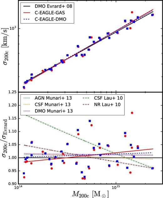
Top panel: the σ200 c–M200 c relation for all 30 C-EAGLE clusters at z = 0. The red solid and dashed blue lines show the best-fitting relation for the DM particles within r200 c for the C-EAGLE-GAS and C-EAGLE-DMO runs, respectively. Similarly, the blue squares and red circles show results for individual clusters in the two simulation sets. The solid black line is the best-fitting relation found by Evrard et al. (2008). Bottom panel: best-fitting relations relative to the Evrard et al. (2008) result. Additionally, the dotted magenta, orange, and cyan lines are the best-fitting results found by Munari et al. (2013) for their DMO, CSF, and AGN runs, respectively, while the burgundy and green dot–dashed lines are for the NR and CSF simulations found by Lau et al. (2010), respectively.
We find that the scatter in the σ200 c–M200 c relation for the C-EAGLE-DMO clusters, δln = 0.048 ± 0.006, is consistent with that found by Lau et al. (2010) for their NR model, δln = 0.041 ± 0.008 and the global relation found by Evrard et al. (2008), δln = 0.043 ± 0.002. We also find that the scatter does not significantly change when baryons are introduced, increasing by one standard deviation from 0.048 ± 0.006 to 0.055 ± 0.007. This is similar to Lau et al. (2010), who find δln = 0.056 ± 0.009 for their CSF simulation. Munari et al. (2013) consistently found the scatter to be ∼0.05 across their DMO, NR, CSF, and AGN runs. These results imply that the scatter is relatively insensitive to any implemented baryonic physics.
In Fig. 2, we also compare σ200 c for individual clusters in the C-EAGLE-GAS and C-EAGLE-DMO simulations. The black circles show the ratio, R, of the C-EAGLE-GAS and C-EAGLE-DMO velocity dispersions versus M200 c (the same result is shown in each panel). The weighted mean ratio is consistent with unity, 〈R〉 = 1.00 ± 0.03. Note that one cluster (CE-27) is an outlier with R = 1.15; this object undergoes a major merger around z = 0.1, however due to timing differences in the simulations this does not happen at precisely the same time in the DMO run, changing the times at which subfind considers the two merging clusters the same. At z = 0.1, the mass ratio is 0.55, increasing to 0.96 at z = 0. Clearly, CE-27 is significantly disturbed at low redshift and so it is not surprising that there is still a discrepancy in the DM velocity dispersion at z = 0.
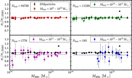
The effect of baryons on the cluster velocity dispersion. Each point shows the ratio of the velocity dispersion for a cluster in the C-EAGLE-GAS to the corresponding object in the C-EAGLE-DMO runs. Black circles are for DM particles within r200 c, which are the same in all panels, while coloured squares correspond to subhaloes/galaxies binned by total mass (one bin per panel). Error bars show one standard deviation from bootstrapping the data 10 000 times. The dashed line represents no change between simulations while the solid line gives the weighted mean for each subhalo mass bin. The total number of galaxies within the C-EAGLE-GAS clusters in the respective total mass range is also given in each panel.
3.2 Velocity bias in galaxies
As the velocity dispersion of the DM is not directly observable, it is important to determine if the galaxies residing within the cluster are reliable tracers of the underlying matter distribution. In order to establish how biases come into play, the galaxies are split into several bins depending on their total mass, MSub, and their stellar mass, M*. We also use the term subhalo to refer to objects in the C-EAGLE-DMO sample and when comparing between the GAS and DMO sample we use subhalo to refer to galaxies selected by total mass.
We first look at how the dynamics of the subhaloes change when baryons are introduced. Each panel in Fig. 2 shows the ratio of the subhalo velocity dispersion in a cluster between the C-EAGLE-GAS and C-EAGLE-DMO runs, for four subhalo mass ranges. (We do not match individual subhaloes between the two simulations of each cluster as this approach is complicated by timing offsets.) We can see from the figure that the introduction of baryonic physics has a mass-dependent effect on the subhaloes. For subhaloes with masses between 109 and 1010 M⊙, we find no statistically significant change in σ200 c. Similarly, for MSub = 1010–1011 M⊙, the average change is 〈R〉 = 0.99 ± 0.012. However, for the higher mass subhaloes, which are in the mass range studied in previous work, there is a decrease in σ200 c of around 5 per cent, and an increase in the cluster-to-cluster scatter with the introduction of baryons. The decrease in σ is also radially dependent, with subhaloes within the inner region (<0.2r200 c) having a lower velocity dispersion in the runs with baryons. Since we know that the central galaxies are too massive in our simulations (Bahé et al. 2017), we refrain from drawing conclusions about the central region of the clusters.
Fig. 3 shows the best-fitting parameter values for the σ200 c–M200 c relation as a function of redshift, for the different subhalo and galaxy mass bins as well as for the DM particles (the z = 0 results for the subhaloes and galaxies are also listed in Table 1).
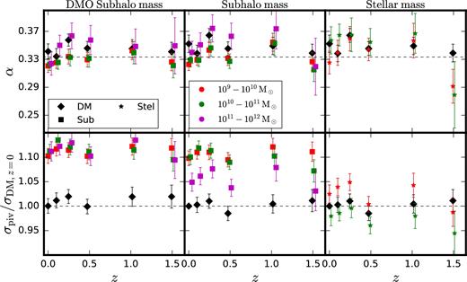
Fitting parameters obtained for equation (2) using galaxies and DM particles. The top row shows the fitted value of logarithmic slope, α, as a function of redshift, while the bottom row shows the values of the normalization σpiv. σpiv is shown relative to the value obtained for the DM particles at z = 0. The expected self-similar value of α = 1/3 is shown by the dashed line in the top row, whereas the dashed lines in the lower panel show now change between the value of σpiv obtained at z = 0 using DM particles. The columns left to right are for the DMO runs, with subhaloes binned by total mass, galaxies binned by total mass in the hydro runs and galaxies binned by stellar mass. The uncertainties are obtained by bootstrap re-sampling the 30 clusters 104 times.
The left and middle columns show the best-fitting parameters for the total mass bins in the C-EAGLE-DMO and C-EAGLE-GAS runs, respectively, whereas the right column shows the best-fitting parameters for the C-EAGLE-GAS galaxies. The logarithmic slope, α, is shown in the top panels, with the dashed horizontal line showing the expected self-similar value of α = 1/3. The lower row shows the normalization, σpiv, relative to the value found for the DM particles in the C-EAGLE-GAS runs at z = 0.
In all cases, the slopes are broadly consistent with the expected self-similar value, although there is a tendency for them to be high, particularly the highest mass subhaloes and galaxies at intermediate redshifts (0.25 < z < 1). However, these deviations do not affect the trends seen in the normalization, as can be deduced from comparing the results in the bottom row of Fig. 3. Our slopes are consistent with those found by Munari et al. (2013) and Caldwell et al. (2016), who obtained slopes of 0.364 ± 0.0021 and 0.385 ± 0.003, respectively, for galaxies with stellar masses ≳1010 M⊙.
When σ200 c is calculated using the DM particles, no systematic deviation from self-similar evolution with redshift is seen for the runs with and without baryons for z < 1.5. This result is consistent with the findings of Munari et al. (2013) and Caldwell et al. (2016), who also find no evolution outside of that expected from self-similar. All subhalo mass bins show a velocity bias of ∼1.1 for the C-EAGLE-DMO simulation that persists to z = 1.5. However, when baryons are included we find the velocity bias decreases for increasing total mass. The smallest mass bins (MSub < 1011 M⊙) have a similar bias to those in C-EAGLE-DMO but the bias reduces to ∼1.05 for the highest mass bin. This trend with total mass persists to higher redshift.
When selecting galaxies by stellar mass the bias is significantly reduced; our results are consistent with no bias at z = 0 for both stellar mass bins considered. There is still a mass trend, with the least massive galaxies having a higher velocity dispersion, and the fitting error is marginally greater relative to the total mass value. Nevertheless, the results obtained suggest that binning the data by stellar mass is a more effective way to reduce the velocity bias between the galaxies and DM particles. This result is in agreement with previous work. As discussed in the introduction, Munari et al. (2013) found a velocity bias of bv = 1.095 when using subhaloes with mass >1011 M⊙ in their full AGN run. When selecting galaxies with stellar mass >3 × 10⁹ M⊙ they obtain a smaller bias of bv = 1.075. While both of these results are higher than what we find for a similar mass range, the trend is the same. A similar result was also found by Lau et al. (2010) for their CSF simulation.
An unexpected result, seen in Table 1, is that the scatter in the σ200 c–M200 c relation is lower (δln ≃ 0.03) for the 109–1011 M⊙ galaxies than for the DM particles (δln ≃ 0.05). This is the case for both the C-EAGLE-GAS and C-EAGLE-DMO runs and does not change when we require that α = 1/3. Munari et al. (2013) found that their subhaloes (with MSub > 1011 M⊙) had a scatter around twice that of the DM particles. We do not find such a large increase in scatter in the 1011–1012 M⊙ mass bin, with an increase in scatter of 45 per cent. Compared to other work, Caldwell et al. (2016) find a total scatter of δln = 0.16 in the high cluster mass regions of their simulation sample, which is higher than our value of δln = 0.11 for a similar mass range. Munari et al. (2013) attempted to separate the intrinsic and statistical components due to scatter and concluded that the subhaloes’ intrinsic scatter was comparable to the DM particles, i.e. if there were significantly more high-mass subhaloes per cluster the scatter would tend to the DM value of ∼5 per cent. Our findings take this further as the galaxies binned by total mass suffer from significantly less scatter than the DM particles, whereas binning in stellar mass results in greater scatter.
The scatter observed in the stellar mass bins, as well as in the 1011–1012 M⊙ total mass bin, is likely affected by statistical noise as there are significantly smaller number of galaxies present in each cluster for those mass ranges. The second column of Table 1 shows the typical number of galaxies, Neff, piv, in each bin for a cluster of mass M200 c = Mpiv = 4 × 10¹⁴ M⊙. We calculate this value by dividing the number of galaxies in each mass bin by the host cluster mass, multiplying by the pivot mass and then taking the median and 68 percentile range. We can see that the number of galaxies in each increasing mass bin decreases by an order of magnitude and so it is not surprising that the scatter is larger for the higher mass bins.
Returning to Fig. 2, we noted that CE-27, which undergoes a major merger at z = 0.1, has a very different DM velocity dispersion between the DMO and GAS simulations. However, the subhalo velocity dispersion has changed far less. We follow up on this observation by splitting the clusters into relaxed and unrelaxed objects, using the relaxation criterion in Barnes et al. (2017b): relaxed clusters are defined as those with Ekin,500 c/Etherm,500 c < 0.1, where Ekin,500 c is the sum of the kinetic energy of the gas particles inside r500 c, excluding any bulk motion, and Etherm, 500 c the sum of the thermal energy of the gas particles. Using this criterion, we find that nine clusters are relaxed at z = 0. Calculating the scatter for the relaxed sample, we find that for the DM particles it decreases from δln = 0.055 ± 0.007 to δln = 0.018 ± 0.003. The scatter in the subhalo and galaxy relations is less affected by selecting only the relaxed clusters, all bins changed by less than one standard deviation when restricting the sample to relaxed clusters. The exception was the 109–1010 M⊙ subhalo bin, which changed from δln = 0.033 ± 0.005 to δln = 0.019 ± 0.004. We conclude that the DM particle velocity dispersion is more susceptible to the past history of the cluster than the subhaloes or galaxies. However, the limited number of galaxies is likely to dominate the measured scatter, rather than the intrinsic variability.
3.3 Stellar mass–total mass relation
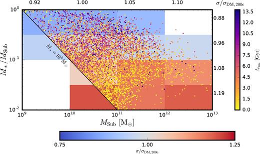
We now seek to understand the underlying reason why the velocity bias differs when binning galaxies by their stellar rather than total mass within r200 c. Fig. 4 shows the stellar mass–total mass relation at z = 0 for all galaxies in the 30 clusters with both MSub > 109 M⊙ and M* > 109 M⊙. The solid, dashed, and dot–dashed diagonal lines correspond to stellar mass fractions of 1, 0.1, and 0.01, respectively. The stellar mass–halo mass relation found by Moster, Naab & White (2013) is also shown as the green solid line, which applies to central galaxies and is therefore not directly comparable with a cluster population. We can see that the qualitative shape of the C-EAGLE distribution is similar to that found by Moster et al. (2013); however, it is offset to larger stellar mass fractions. This result is discussed in more detail in Bahé et al. (2017), who found this offset to persist to at least 10r200 c.
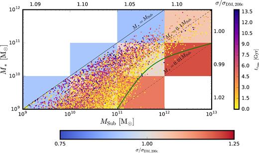
Stellar mass versus total mass for galaxies within r200 c from all 30 clusters. The colour of each point denotes the time since the galaxy first crossed r200 c, where a galaxy with |$t_\mathrm{r_{200{\, }c}\,=\,}0$| has only just entered the cluster. The colour grid behind the points illustrates the velocity bias of the galaxies in each 2D bin, while values on the top (right) give the bias for all objects within each total (stellar) mass bin (errors are typically ±0.01). The black solid, dashed, and dot–dashed lines show stellar mass fractions of 1, 0.1, and 0.01, respectively. The green solid line shows the stellar mass–halo mass relation from Moster et al. (2013).
A significant driver of the scatter in the stellar mass fraction is the time a galaxy has resided within the cluster. We use the merger trees to trace the main progenitors of the galaxies back in time until they first crossed r200 c(z); we define this time as |$t_{r_{\rm 200{\, }c}}$|, so that newly entered galaxies have |$t_{r_{\rm 200{\, }c}} = 0 {\, } \mathrm{Gyr}$|. Older galaxies, i.e. with a larger |$t_{r_{\rm 200{\, }c}}$|, tend to have a higher stellar mass fraction. This is because the DM is more diffuse than the stellar component and so is more easily stripped due to dynamical processes as the galaxy orbits within the cluster potential.
The velocity bias of all galaxies with respect to the DM particles in their host cluster is also shown in Fig. 4. To calculate this, we first scale out the cluster mass dependence by dividing the velocity of each galaxy by the velocity dispersion of the DM particles in its host halo. The overall bias, calculated as a 2D distribution of both total and stellar mass, is shown in the background grid, with blue (red) regions corresponding to smaller (larger) velocity dispersions than the DM particles. We also give values of the bias for each mass bin along the top (right) of the figure. For these, all galaxies in the mass bin are taken into account, not just those with masses above 109 M⊙ as shown. This is done to be more consistent with the values in Table 1.
There is a clear trend that galaxies that have been inside the cluster longer (and thus have a stellar mass fraction closer to unity) have an accordingly lower velocity dispersion. Fig. 4 also shows the reduced velocity bias when binning by stellar, rather than total, mass, denoted by the values on the edge of the plot. To understand why the velocity bias is reduced, consider a toy model of a cluster where all galaxies have the same stellar mass fraction upon entering. Galaxies begin to spread out along the MSub direction only as the stellar mass of a galaxy does not begin to be stripped until a significant fraction (∼80 per cent) of the surrounding DM has been lost (Smith et al. 2016), due to the stellar component residing much deeper in the subhalo potential. Hence, by selecting objects based on stellar mass one obtains a fairer sample of tracers, with each object at a different point in their dynamical history. Contrast this with slices along the MSub axis, where there will now be a mix of galaxies that are young (with a low stellar mass fraction) and old (with a high stellar mass fraction). Crucially, their dynamical histories (past and future) will be different as this depends on their total mass when they first entered the cluster. Furthermore, due to the steepness of the halo-mass function, results are biased towards newly entered, dynamically hot galaxies when binning in total mass. This does not occur for stellar mass bins as a subhalo will tend to stay within that bin until close to the end of its life, when the stars eventually become stripped. The key point is that selecting galaxies by total mass results in a younger population in a given mass range compared to selecting by stellar mass. When selecting by stellar mass, the older galaxies, which have been slowing down due to dynamical friction, happen to compensate for the young hot galaxies, reducing the bias.
We show the correlation between stellar mass fraction, age, and velocity bias more clearly in Fig. 5 where we have plotted stellar mass fraction against total mass. One can clearly see the change in bias as one moves from older, colder galaxies with a high stellar mass fraction down to younger galaxies with lower stellar mass fractions. We only show galaxies with a stellar mass greater than 109 M⊙ as the EAGLE model was not calibrated to reproduce the galaxy population below this threshold. The change in the bias at low masses between here and in Fig. 4 is due to this stellar mass cut preferentially.
Stellar mass fraction versus total mass for galaxies within r200 c from all 30 clusters. Only galaxies with a stellar mass greater than 109 M⊙ are shown. The layout is the same as in Fig. 4.
Binning galaxies by their stellar mass fraction does not reduce the scatter in the σ–M relation compared to the stellar mass case as Neff,piv = 58 and 77 for the [0.01, 0.1] and [0.1, 1] stellar mass fraction bins, respectively. These numbers are similar to the case for the stellar mass bins and so the scatter is also similar, with δln = 0.11 ± 0.01 and 0.056 ± 0.006, respectively. We conclude that any reduction in the intrinsic scatter is masked by the limited number of galaxies per cluster.
In addition to binning galaxies by their stellar mass, we also binned galaxies by their internal stellar velocity dispersion, ςgal,*, and their maximum circular velocity, Vc, Max. The fitting relations obtained when binning galaxies by ςgal,* and Vc,Max are given in Table A3. We find that binning by ςgal,* also returns an unbiased velocity dispersion. We conclude that selecting galaxies based on properties that are not significantly affected by entering the cluster environment is effective in mitigating the effects of velocity bias.
3.4 Velocity bias and dynamical history
We also need to explain the trend seen in Fig. 4 between stellar mass fraction and velocity bias. To do this, we examine the dynamical history of the galaxies in more detail. We remind the reader that we define the time passed since a galaxy first entered inside r200 c(z) of the main cluster as |$t_{r_{\rm 200{\, }c}}$|, so that a galaxy that entered at the present day has |$t_{r_{\rm 200{\, }c}}=0$|.
Fig. 6 shows the radial positions of all galaxies in CE-26 at z = 0 that had a total mass MSub > 109 M⊙ when they first entered r200 c of the main halo, as a function of |$t_{r_{\rm 200{\, }c}}$|.5 On the basis that these positions are sampling typical orbital trajectories, we see that the vast majority of subhaloes will go beyond r200 c after their first infall. However, when the galaxies fall back on to the cluster their motions are less coherent. (Note that the striping seen for |$t_{r_{\rm 200{\, }c}}>7 {\, } \mathrm{Gyr}$| is due to the finite number of outputs from the simulation.) Recent work by Rhee et al. (2017) found a similar structure when analysing subhalo positions in phase space as a function of time. Rhee et al. (2017) found very weak dependence on galaxy and host cluster mass, and we find the same qualitative structure across the whole mass range of clusters studied in the C-EAGLE-GAS sample.
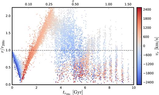
Radial positions of all galaxies at z = 0 with MSub > 109 M⊙ in CE-26 against time of first crossing r200 c. Colours indicate the radial velocity of each subhalo with respect to the cluster centre and the dashed line is r200 c at z = 0. The velocity dispersion of the DM particles inside r200 c is 1119 km s−1 at z = 0.
The top panel of Fig. 7 shows the ratio of galaxy’s total mass at z = 0 to that at |$t_{r_{\rm 200{\, }c}}$|, versus |$t_{r_{\rm 200{\, }c}}$|. As expected, older galaxies have lost more mass. For example, after ∼10 Gyr in a cluster, a galaxy will have lost 60–70 per cent of its initial mass. The results are split across three total mass bins (measured at |$t_{r_{\rm 200{\, }c}}$|). There is little, if any, total mass dependence for the proportional rate of mass-loss when a galaxy enters a cluster, although the results are biased towards those that have survived until the present day. We find the rate of mass-loss to be broadly similar to that found by Joshi, Wadsley & Parker (2017).
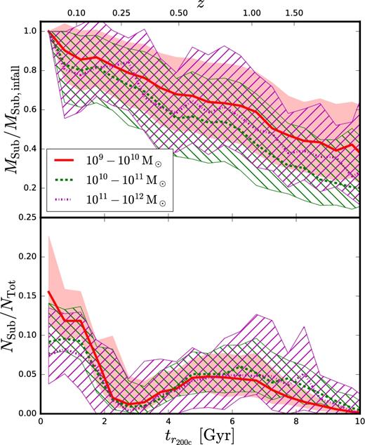
Top panel: ratio of a galaxy’s present (z = 0) mass to its mass when it first crossed r200 c. Bottom panel: fraction of galaxies inside r200 c at z = 0 that fell into the cluster at |$t_{r_{\rm 200{\, }c}}$|. Results in both panels are plotted against |$t_{r_{\rm 200{\, }c}}$|. The median values for all 30 clusters are shown as the bold lines with shaded regions depicting the 16th and 84th percentiles. Galaxies are binned with respect to their total mass at infall.
The bottom panel of Fig. 7 shows the median fraction of galaxies as a function of |$t_{r_{\rm 200{\, }c}}$|, averaged across all 30 clusters. As expected from Fig. 6, there is a deficit of galaxies that first crossed r200 c ∼3 Gyr ago, as most of those galaxies are now beyond r200 c. We also see a slight total mass dependence, with a greater of proportion of the lower mass 109–1010 M⊙ galaxies entering the cluster more recently than the higher mass 1011–1012 M⊙ galaxies. This is expected as lower mass galaxies are closer to the resolution limit of the simulation and so are less likely to survive until the present day.
In Fig. 8, we show how the velocity bias, estimated from stacking all 30 clusters together, depends on infall time. Again, we do this by normalizing the velocity of each galaxy to the velocity dispersion of the DM particles in its host halo; the galaxies are also split into three bins of varying total mass at infall.
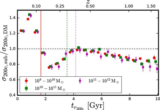
Velocity bias of galaxies inside r200 c at z = 0 shown as a function of time spent in the cluster. The velocities of the galaxies were divided by the velocity dispersion of the host cluster and all galaxies were then binned by their infall total mass. The error bars correspond to ±1 standard deviation, obtained by bootstrap re-sampling 10 000 times. The vertical solid, dashed, and dot–dashed lines show the median value of |$t_{r_{\rm 200{\, }c}}$| for the low, middle, and high-mass bins, respectively.
There are three key stages in this plot. First, galaxies that entered the cluster in the last 2 Gyr have a high velocity dispersion compared to the DM particles in their host cluster (i.e. bv > 1), with the peak bias coinciding with the point where they have had time to reach the pericentre of their first orbit (see Fig. 6). Secondly, galaxies that entered between 2 and 4 Gyr ago are biased low (bv < 1); this corresponds to the minimum in the galaxy fraction, shown in the lower panel of Fig. 7. Most of these galaxies have gone beyond r200 c, with only the slower objects, or those on more circular orbits, remaining. Finally, at 4 Gyr, we see that bv ≃ 1 and then a smooth trend towards a lower velocity bias with age, as the process of dynamical friction gradually slows the galaxies down.
Fig. 8 also implies that there is little total mass dependence in the slowdown of galaxies in the cluster when considering the last ∽9 Gyr, contrary to what one might expect from analytical models (Chandrasekhar 1943; Adhikari, Dalal & Clampitt 2016). Instead, the velocity bias originates from the distribution of galaxies as a function of |$t_{r_{\rm 200{\, }c}}$|. The vertical lines in Fig. 8 show the median values of |$t_{r_{\rm 200{\, }c}}$| for the three mass bins, highlighting the total mass dependence seen in the lower panel of Fig. 7: lower mass galaxies tend to be younger than their higher mass counterparts. As the galaxies are only positively biased on their first pass through a cluster, the lower the |$t_{r_{\rm 200{\, }c}}$|, the higher the velocity bias. When |$t_{r_{\rm 200{\, }c}}>9 {\, } \mathrm{Gyr}$|, we do see signs of a total mass dependence in the velocity bias, with the velocity dispersion of the highest mass subhaloes decreasing faster than the others. The same qualitative shape shown in Fig. 8 has also been observed in Ye et al. (2017) using the Illustris simulations.
We finally look at how the different components (radial and angular co-ordinates: r, θ, ϕ) of the galaxy’s velocity depend on |$t_{r_{\rm 200{\, }c}}$|. Fig. 9 shows the median velocity component (vi; top panel), and velocity dispersion component (σi; lower panel) as a function of |$t_{r_{\rm 200{\, }c}}$| for all galaxies in the 30 clusters with MSub > 109 M⊙. The galaxy velocities are scaled by the velocity dispersion of the DM particles.
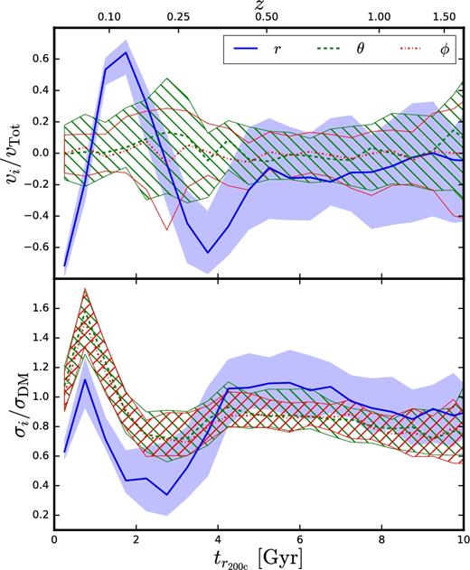
Radial and tangential velocity components (top panel) and velocity dispersion components (lower panel) for galaxies in all 30 clusters versus infall time, |$t_{r_{\rm 200{\, }c}}$|. Bold lines show the median values while the corresponding hatched regions represent the cluster-to-cluster scatter (±1 standard deviation). The results are normalized to the velocity dispersion of the DM particles.
As expected, the tangential velocity components approximately average to zero and only the radial component has a strong directional preference over the last 4 Gyr. We can also see that there is very little spread between clusters in terms of their radial velocity before ∼4 Gyr, as the majority of galaxies are at the same point in their orbit. The velocity dispersion of each component, shown in the lower panel of Fig. 9, shows the same trend as Fig. 8. However, we see that the dispersion of the radial component is below the two tangential components for |$t_{r_{\rm 200{\, }c}}<4 {\, } \mathrm{Gyr}$|. Again, this is due to all of the galaxies accelerating towards the centre of the cluster (or being decelerated as they move outwards), reducing the width of the velocity distribution, whereas the tangential components have no reason to be aligned by this effect.
3.5 Dependence on aperture size
Throughout this paper, we have focused on the velocity dispersion inside r200 c. We now present results for two other common apertures, r500 c and r200 m, where the latter is defined relative to the mean density rather than the critical density. Fig. 10 shows the median cumulative σ profiles, normalized to the cumulative velocity dispersion of the DM particles, using all galaxies within a given radius. We can see that the σ(<r)/σ(<r)DM ratio changes significantly less when the galaxies are binned by stellar mass compared to total mass. We quantify this by calculating the σ–M relation at r500 c and r200 m, the parameters of which are given in Table. 2, where we have duplicated the relevant parameters for r200 c for ease of comparison.
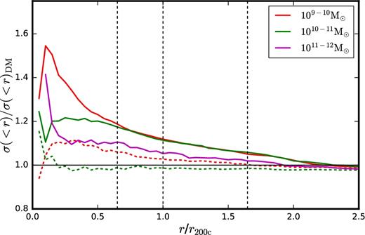
The cumulative velocity dispersion of the galaxies binned by total mass (solid lines) and stellar mass (dashed lines) as a function of distance from the cluster, relative to the cumulative velocity dispersion of the DM particles. The radial distance is in units of r200 c, with medium values of r500 c and r200 m denoted by the vertical black dashed lines, respectively, as well as r200 c. The coloured lines show the median values for the 30 clusters.
Best-fittingparameters for the σ–M relation, for DM particles and galaxy total/stellar mass bins within r500 c, r200 c, and r200 m at z = 0. Symbols have the same meanings as in Table 1.
| r500 c | α | σpiv (km s−1) | σpiv/σpiv, DM |
|---|---|---|---|
| DM particles | 0.36 ± 0.01 | 958 ± 9 | |
| MSub | |||
| 109–1010 M⊙ | 0.33 ± 0.01 | 1101 ± 8 | 1.15 ± 0.01 |
| 1010–1011 M⊙ | 0.33 ± 0.01 | 1093 ± 9 | 1.14 ± 0.01 |
| 1011–1012 M⊙ | 0.33 ± 0.02 | 1037 ± 13 | 1.08 ± 0.02 |
| M* | |||
| 109–1010 M⊙ | 0.32 ± 0.01 | 992 ± 9 | 1.04 ± 0.01 |
| 1010–1011 M⊙ | 0.36 ± 0.02 | 941 ± 12 | 0.98 ± 0.02 |
| r200 c | |||
| DM particles | 0.35 ± 0.01 | 804 ± 9 | |
| MSub | |||
| 109–1010 M⊙ | 0.32 ± 0.01 | 883 ± 7 | 1.10 ± 0.01 |
| 1010–1011 M⊙ | 0.33 ± 0.01 | 885 ± 8 | 1.10 ± 0.02 |
| 1011–1012 M⊙ | 0.34 ± 0.02 | 844 ± 11 | 1.05 ± 0.02 |
| M* | |||
| 109–1010 M⊙ | 0.32 ± 0.02 | 823 ± 11 | 1.02 ± 0.02 |
| 1010–1011 M⊙ | 0.36 ± 0.02 | 789 ± 13 | 0.98 ± 0.02 |
| r200 m | |||
| DM particles | 0.35 ± 0.01 | 683 ± 8 | |
| MSub | |||
| 109–1010 M⊙ | 0.335 ± 0.009 | 710 ± 6 | 1.04 ± 0.02 |
| 1010–1011 M⊙ | 0.344 ± 0.009 | 710 ± 6 | 1.04 ± 0.02 |
| 1011–1012 M⊙ | 0.34 ± 0.01 | 690 ± 10 | 1.01 ± 0.02 |
| M* | |||
| 109–1010 M⊙ | 0.33 ± 0.02 | 684 ± 11 | 1.00 ± 0.02 |
| 1010–1011 M⊙ | 0.35 ± 0.02 | 663 ± 14 | 0.97 ± 0.02 |
For the three apertures in Table 2, we can see that σpiv/σpiv, DM changes substantially more as a function of radius for the two lowest total mass bins than for the stellar mass bins. Beyond 2r200 c there is very little, if any, bias; when selecting by either total or stellar mass, one would expect the bias to lessen with distance as processes such as dynamical friction will not be acting to the same degree as inside the cluster. Qualitatively, we see the same features in the σ–M relation for the three apertures; selecting galaxies by total mass results in a positive velocity bias, whereas the more observationally motivated selection by stellar mass yields little ( < 5 per cent) to no bias on average.
4 DISCUSSION AND CONCLUSIONS
We have used the C-EAGLE simulations (Bahé et al. 2017; Barnes et al. 2017b) to explore the extent and nature of the velocity bias introduced when using galaxies as dynamical tracers of the underlying cluster potential. The simulations are amongst the highest resolution cosmological simulations of galaxy clusters run to date (1 kpc force resolution at z ≈ 0) and adopt a subgrid physics prescription that has been calibrated to produce the stellar mass functions, sizes, and black hole masses of field galaxies (Crain et al. 2015; Schaye et al. 2015). Recent work has also demonstrated that the C-EAGLE simulations approximately reproduce key properties of the galaxies (Bahé et al. 2017) and hot gas (Barnes et al. 2017b) in cluster environments.
In line with other recent work, we have found that DMO subhaloes have a velocity dispersion that is around 5–10 per cent higher than the DM particles within r200 c. However, this bias is significantly reduced when selecting galaxies in hydrodynamical simulations based on their observational properties such as stellar mass or stellar velocity dispersion. This finding has only been possible because of the high resolution of the C-EAGLE galaxies, where the stellar component, located at the subhalo centre of potential, is more robust to stripping effects than the surrounding DM component. This may explain the difference between our results and those of other groups such as Munari et al. (2013), who found a similar bias when binning in total and stellar mass.
Our main findings can be summarized as follows.
The intrinsic velocity dispersion of the DM particles in a cluster is tightly correlated with cluster mass, with and without the inclusion of baryonic physics (Fig. 1). The relation obtained in this paper is consistent with previous work by Evrard et al. (2008) and Munari et al. (2013).
In the C-EAGLE-DMO simulations, the velocity dispersion of subhaloes has a relatively constant bias, ∼10 per cent above the DM particle value, regardless of subhalo mass (109 < MSub/M⊙ < 1012) or redshift (0 ≤ z ≤ 1.5). The inclusion of baryonic physics has little effect on the velocity dispersion of low-mass galaxies but higher mass (>1011 M⊙) galaxies have their bias reduced to around 5 per cent (Fig. 3).
The velocity bias is suppressed to within a few per cent when selecting galaxies based on their stellar mass instead of their total mass (Fig. 3). This difference arises from having a larger fraction of galaxies that have newly entered the cluster when selecting by total mass; these galaxies tend to be hotter than objects that have been in the cluster for longer (Figs 4 and 5).
We find that the fractional mass-loss of galaxies has an approximately linear trend with the time spent in the cluster, with little dependence on the cluster or total mass, in agreement with Joshi et al. (2017) and Rhee et al. (2017). We also find that a marginally larger fraction of low-mass galaxies have newly entered the clusters relative to high-mass galaxies. This would be expected partly due to the limitations of subfind not being able to reliably identify galaxies ≲108 M⊙ (Fig. 7) (Muldrew, Pearce & Power 2011).
Figs 6 and 7 can be used together to explain why velocity bias has a strong dependence on infall time, |$t_{r_{\rm 200{\, }c}}$|, as shown in Fig. 8. Galaxies on their first pass through a cluster are on highly radial orbits, with the peak in velocity dispersion occurring closest to the pericentre, i.e. the cluster centre. Once the galaxies enter r200 c for the second time, they are approximately unbiased and their velocity dispersion steadily decreases due to dynamical friction thereafter.
The velocity bias varies more strongly as a function of distance from the centre of the cluster when binning galaxies by total mass compared to stellar mass. At r500c, r200 c, and r200 m, binning galaxies by stellar mass results in a bias of less than 5 per cent (Fig. 10).
In conclusion, we find that the velocity bias of cluster galaxies within r200 c is small, bv = 1 ± 0.05, out to beyond z = 1, so long as the galaxies are selected by their (observable) stellar mass or velocity dispersion. This has promising implications for cluster cosmology where a growing number of new spectroscopic surveys will be used to measure cluster masses via galaxy kinematics, e.g. using the caustic method (Diaferio & Geller 1997; Gifford, Kern & Miller 2017).
In future work, we plan to use the C-EAGLE cluster sample to investigate the reliability of caustic mass estimates. We will also simulate observations of these clusters to establish how observational considerations such as line-of-sight contamination, selection bias, and projection effects affect the results, as well as how more observationally expensive techniques can be combined with the σ–M relation to yield tighter mass constraints.
Acknowledgements
We would like to thank Ian McCarthy and Joop Schaye for their helpful comments on the initial manuscript. This work used the DiRAC Data Centric system at Durham University, operated by the Institute for Computational Cosmology on behalf of the STFC DiRAC HPC Facility (www.dirac.ac.uk). This equipment was funded by BIS National E-infrastructure capital grant ST/K00042X/1, STFC capital grants ST/H008519/1 and ST/K00087X/1, STFC DiRAC Operations grant ST/K003267/1, and Durham University. DiRAC is part of the National E-Infrastructure. The Hydrangea simulations were in part performed on the German federal maximum performance computer ‘HazelHen’ at the maximum performance computing centre Stuttgart (HLRS), under project GCS-HYDA/ID 44067 financed through the large-scale project ‘Hydrangea’ of the Gauss Center for Supercomputing. Further simulations were performed at the Max Planck Computing and Data Facility in Garching, Germany. We also gratefully acknowledge PRACE for awarding the EAGLE project access to the Curie facility based in France at Trés Grand Centre de Calcul. DJB and STK acknowledge support from STFC through grant ST/L000768/1. TJA is supported by an STFC studentship.
Footenotes
We define M200 c as the mass enclosed within a sphere of radius r200 c whose mean density is 200 times the critical density of the universe.
A DMO version of each cluster was also run to quantify the effect of introducing baryons. For these runs, the particle mass was set to 1.15 × 10⁷ M⊙. We refer to these clusters collectively as C-EAGLE-DMO.
The snapshots were spaced 500 Myr apart, with two additional outputs at z = 0.1 and 0.37 for comparison with the original EAGLE simulations.
We have also performed the analysis using the bi-weight estimator, as suggested by Beers et al. (1990) for large data sets. We found little change in the results and so only present the results from the gapper method in this paper.
Fig. 6 is qualitatively representative of what is observed across most clusters. Clusters that have recently undergone a major merger show a more complex structure.
REFERENCES
APPENDIX: ADDITIONAL CLUSTER PROPERTIES
In this appendix, we list additional cluster properties that the reader may find useful. In Table A1, we list the measured velocity dispersions of the DM particles within r200 c for each C-EAGLE cluster at z = 0. These are presented alongside r200 c, M200 c, and the size of the high-resolution region. The table can be used in conjunction with additional data presented in Bahé et al. (2017) and Barnes et al. (2017b).
Global properties of the C-EAGLE clusters at z = 0, used in this paper. The velocity dispersion σ200 c is calculated using only the DM particles inside r200 c. rclean is the maximum radius containing only high-resolution particles.
| Halo | r200 c (Mpc) | M200 c (M⊙) | σ200 c (km s−1) | rclean/r200 c |
|---|---|---|---|---|
| CE-00 | 1.04 | 1.19 × 10¹⁴ | 457 | 5 |
| CE-01 | 1.02 | 1.15 × 10¹⁴ | 425 | 5 |
| CE-02 | 1.05 | 1.22 × 10¹⁴ | 462 | 5 |
| CE-03 | 1.08 | 1.36 × 10¹⁴ | 476 | 5 |
| CE-04 | 1.19 | 1.78 × 10¹⁴ | 544 | 5 |
| CE-05 | 1.09 | 1.38 × 10¹⁴ | 517 | 5 |
| CE-06 | 1.27 | 2.20 × 10¹⁴ | 548 | 10 |
| CE-07 | 1.27 | 2.17 × 10¹⁴ | 553 | 10 |
| CE-08 | 1.30 | 2.37 × 10¹⁴ | 584 | 5 |
| CE-09 | 1.39 | 2.86 × 10¹⁴ | 633 | 5 |
| CE-10 | 1.40 | 2.94 × 10¹⁴ | 617 | 5 |
| CE-11 | 1.44 | 3.19 × 10¹⁴ | 682 | 5 |
| CE-12 | 1.55 | 3.96 × 10¹⁴ | 683 | 10 |
| CE-13 | 1.57 | 4.11 × 10¹⁴ | 768 | 10 |
| CE-14 | 1.62 | 4.55 × 10¹⁴ | 672 | 10 |
| CE-15 | 1.71 | 5.31 × 10¹⁴ | 737 | 10 |
| CE-16 | 1.74 | 5.62 × 10¹⁴ | 880 | 10 |
| CE-17 | 1.65 | 4.78 × 10¹⁴ | 682 | 5 |
| CE-18 | 1.87 | 6.94 × 10¹⁴ | 849 | 10 |
| CE-19 | 1.86 | 6.84 × 10¹⁴ | 868 | 5 |
| CE-20 | 1.77 | 5.96 × 10¹⁴ | 823 | 5 |
| CE-21 | 2.00 | 8.55 × 10¹⁴ | 873 | 5 |
| CE-22 | 2.14 | 1.04 × 10¹⁴ | 938 | 10 |
| CE-23 | 1.99 | 8.39 × 10¹⁴ | 936 | 5 |
| CE-24 | 2.27 | 1.24 × 10¹⁵ | 1107 | 10 |
| CE-25 | 2.36 | 1.40 × 10¹⁵ | 1005 | 10 |
| CE-26 | 2.39 | 1.45 × 10¹⁵ | 1119 | 5 |
| CE-27 | 2.39 | 1.46 × 10¹⁵ | 1264 | 5 |
| CE-28 | 2.50 | 1.67 × 10¹⁵ | 1178 | 10 |
| CE-29 | 2.82 | 2.39 × 10¹⁵ | 1223 | 10 |
Table A2 shows the fitting parameters as in Table 1 but with α fixed to the self-similar value of 1/3. We find no significant change in the normalization, scatter or bias when the gradient is fixed.
Best-fittingparameters to the σ200 c–M200 c relation for the DM particles and galaxies at z = 0 with the logarithmic slope, α, fixed to the self-similar value of 1/3. Column 1 lists the simulation and sample details (with mass limits where appropriate). Columns 2 and 3 give the best-fitting normalization and scatter. Finally, Column 4 gives the ratio of the normalization to the case for DM particles, a measure of the velocity bias for the galaxies.
| σpiv (km s−1) | δln | σpiv/σpiv, DM | |
|---|---|---|---|
| C-EAGLE-DMO | |||
| DM particles | |$803 \pm 7\phantom{0}$| | 0.048 ± 0.006 | |
| MSub: 109–1010 M⊙ | |$882 \pm 6\phantom{0}$| | 0.036 ± 0.005 | 1.10 ± 0.01 |
| MSub: 1010–1011 M⊙ | |$891 \pm 6\phantom{0}$| | 0.035 ± 0.005 | 1.11 ± 0.01 |
| MSub: 1011–1012 M⊙ | 891 ± 10 | 0.061 ± 0.008 | 1.11 ± 0.02 |
| C-EAGLE-GAS | |||
| DM particles | |$800\pm 9\phantom{0}$| | 0.058 ± 0.007 | |
| MSub: 109–1010 M⊙ | |$880\pm 6\phantom{0}$| | 0.034 ± 0.005 | 1.10 ± 0.01 |
| MSub: 1010–1011 M⊙ | |$883\pm 6\phantom{0}$| | 0.035 ± 0.004 | 1.10 ± 0.02 |
| MSub: 1011–1012 M⊙ | 847 ± 10 | 0.09 ± 0.02 | 1.06 ± 0.02 |
| M* : 109–1010 M⊙ | 820 ± 10 | 0.062 ± 0.007 | 1.02 ± 0.02 |
| M* : 1010–1011 M⊙ | 796 ± 11 | 0.11 ± 0.02 | 1.00 ± 0.02 |
In Table A3, we show the best-fitting parameters when binning galaxies by their stellar velocity dispersion ςgal,* as well as their maximum circular velocity, Vc,Max, within r200 c. In general, the results show a similarly small bias as with the stellar mass bins.
Best-fittingσ–M parameters for the subhaloes when binned by stellar velocity dispersion and maximum circular velocity.
| r200 c | α | σpiv (km s−1) | σpiv/σpiv, DM |
|---|---|---|---|
| ςgal, * : 50–100 km s−1 | 0.33 ± 0.02 | 825 ± 14 | 1.03 ± 0.02 |
| ςgal, * : |$100 \!{-}\! 150 \mathrm{{\, } \mathrm{km{\, }s^{-1}}}$| | 0.36 ± 0.03 | 779 ± 18 | 0.97 ± 0.03 |
| ςgal, * : |$150 \!{-}\! 200 \mathrm{{\, } \mathrm{km{\, }s^{-1}}}$| | 0.36 ± 0.05 | 828 ± 32 | 1.03 ± 0.04 |
| Vc,Max : |$50 \!{-}\! 100 \mathrm{{\, } \mathrm{km{\, }s^{-1}}}$| | 0.33 ± 0.01 | 876 ± 9 | 1.09 ± 0.02 |
| Vc,Max : |$100 \!{-}\! 150 \mathrm{{\, } \mathrm{km{\, }s^{-1}}}$| | 0.34 ± 0.02 | 835 ± 14 | 1.04 ± 0.02 |
| Vc,Max : |$150 \!{-}\! 200 \mathrm{{\, } \mathrm{km{\, }s^{-1}}}$| | 0.32 ± 0.03 | 814 ± 18 | 1.02 ± 0.03 |
| Vc,Max : |$200 \!{-}\! 250 \mathrm{{\, } \mathrm{km{\, }s^{-1}}}$| | 0.40 ± 0.03 | 750 ± 20 | 0.94 ± 0.03 |
