


Abstract
Variability and mass-loss are common phenomena in massive OB-type stars. It is argued that they are caused by violent strange mode instabilities identified in corresponding stellar models. We present a systematic linear stability analysis with respect to radial perturbations of massive OB-type stars with solar chemical composition and masses between 23 and 100 M⊙. For selected unstable stellar models, we perform non-linear simulations of the evolution of the instabilities into the non-linear regime. Finite amplitude pulsations with periods in the range between hours and 100 d are found to be the final result of the instabilities. The pulsations are associated with a mean acoustic luminosity which can be the origin of a pulsationally driven wind. Corresponding mass-loss rates lie in the range between 10−9 and 10−4 M⊙ yr−1 and may thus affect the evolution of massive stars.
1 INTRODUCTION
Spectroscopic and photometric variability is a common phenomenon in OB-type stars (see e.g. Lucy 1976; van Genderen 1985; Balona 1992; De Cat et al. 2007). Recently, Laur et al. (2017) have investigated stellar variability within young open star clusters and identified α Cyg, β Cep and slowly pulsating B variables. Concerning low-metallicity environments, Kourniotis et al. (2014) have studied photometric variability of 4646 massive stars in the Small Magellanic Cloud and reported the presence of regular and irregular variabilities in many OB-type stars considered in their sample. A similar study for the Large Magellanic Cloud has been performed by Szczygieł et al. (2010). The origin as well as the mechanism responsible for the variability are still a matter of debate. Among other possible explanations, pulsations have been suggested as the cause of variability in massive stars (see e.g. Lucy 1976; Fullerton, Gies & Bolton 1996).
Similar to variability, mass-loss is a common phenomenon in massive stars from the main sequence to advanced evolutionary stages. Mass-loss is an important still not sufficiently understood ingredient for stellar evolution with consequences even for the galactic environment. Accordingly, it has been the subject of a number of studies (see e.g. the reviews on mass-loss by Puls, Vink & Najarro 2008; Smith 2014). Lucy & Solomon (1970) proposed line driven winds (where the photon momentum is transferred to the gas in the envelope) as the mechanism responsible for mass-loss in OB-type stars. However, episodes of enhanced, strong mass-loss and eruptions observed, e.g. in luminous blue variables are not satisfactorily explained on the basis of line-driven winds. Meanwhile, there is growing evidence for a connection between variability, pulsations and mass-loss (see e.g. Glatzel et al. 1999; Townsend 2007; Kraus et al. 2015; McDonald & Zijlstra 2016; Yadav & Glatzel 2016).
With respect to an explanation and understanding of the observed variability, linear stability analyses have been performed for models of massive stars. They cover main sequence models (Glatzel & Kiriakidis 1993a) and models in advanced evolutionary stages (Wood & Olivier 2014; Jeffery & Saio 2016) and consider stability with respect to both radial and non-radial perturbations (Osaki 1975; Saio & Cox 1980; Glatzel & Mehren 1996). As a result, violent instabilities with growth rates in the dynamical range have been identified, which are associated with the occurrence of strange modes. This type of instability has previously been found in models of hydrogen deficient carbon (see e.g. Wood 1976; Saio, Wheeler & Cox 1984; Gautschy & Glatzel 1990b; Glatzel & Gautschy 1992) and Wolf–Rayet stars (Glatzel, Kiriakidis & Fricke 1993). For the mechanism of strange mode instabilities, we refer to Glatzel (1994), Papaloizou et al. (1997) and Saio, Baker & Gautschy (1998).
Concerning radial perturbations, numerical simulations of the evolution of strange mode instabilities into the non-linear regime show (Glatzel et al. 1999; Yadav & Glatzel 2016) that they can drive episodes of enhanced mass-loss and eruptions. In a recent study (Yadav & Glatzel 2017), we have performed a stability analysis of models for massive zero-age main sequence (ZAMS) stars having solar chemical composition in the mass range between 50 and 150 M⊙. The linear analysis reveals that models having masses above 58 M⊙ are violently unstable. Non-linear simulations show that the instabilities lead to finite amplitude pulsations with periods in the range between 3 and 24 h. The pulsations are associated with a mean acoustic luminosity which might be the origin of pulsationally driven mass-loss and allows for an estimate of the mass-loss rate. For the models considered, the maximum mass-loss rate estimated is found to be of the order of 10−7 M⊙ yr−1.
In this paper, we intend to extend the previous study of Yadav & Glatzel (2017) to post main sequence models, i.e. to models of massive OB-type stars for the same, solar, chemical composition. After construction of stellar models, we shall test them for linear stability to identify unstable models. For selected unstable models, we then perform numerical simulations of the instabilities into the non-linear regime to determine their final result. The paper falls into five sections: stellar models are discussed in Section 2, the linear stability analysis is described in Section 3 and non-linear simulations are presented in Section 4. Our conclusions follow (Section 5).
2 STELLAR MODELS
To study instabilities and pulsationally driven mass-loss, we have considered a wide range of stellar models having properties close to that of OB-type stars. For illustration, the evolutionary tracks from the main sequence to the Hayashi line are shown in Fig. 1 for initial masses of 30, 45, 70 and 100 M⊙, respectively, and solar chemical composition. These tracks have been created using the ‘mad star EZ-Web’ code.1 Effective temperatures, luminosities and masses obtained in this way have been used later on to construct high-resolution envelope models. Since the minimum effective temperature for B-type stars lies around 10 000 K, this study is restricted to models having effective temperatures above this value. Energy transport by convection becomes significant in stellar models having effective temperatures below 10 000 K. In order to avoid difficulties with the treatment of convection, in particular with the still poorly understood coupling of pulsation and convection we will not consider models with effective temperature below 10 000 K. We can then assume that energy transport is dominated by radiation diffusion. For illustration, the ratio of convective and total luminosities is displayed in Fig. 2 for selected models. We deduce that the contribution of the convective luminosity to the total luminosity can become as high as 45 per cent for models having effective temperatures close to 10 000 K.
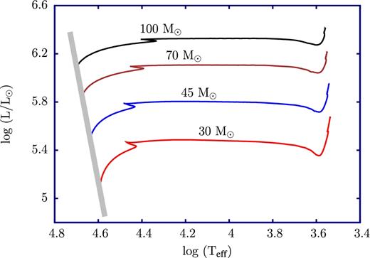
HR diagram of evolutionary tracks with solar chemical composition and the initial masses indicated.
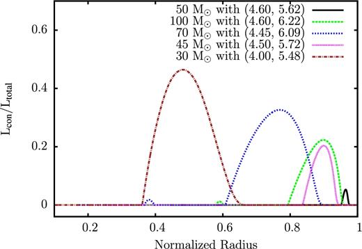
Fraction of convective luminosity as a function of normalized radius for selected models along the evolutionary tracks shown in Fig. 1. The values of log Teff and log L/L⊙ are indicated in brackets.
Since the dynamical instabilities in models of OB-type stars found by Glatzel & Kiriakidis (1993a) are restricted to the envelopes of these objects, the stellar cores may be disregarded for their investigation. Therefore, in this study, we have restricted ourselves to considering the envelopes of OB-type stellar models only. Using effective temperatures, luminosities and masses from the evolutionary calculations for 30, 45, 70 and 100 M⊙, highly resolved envelope models have been constructed as the basis for the subsequent linear stability analysis. These sets of stellar models will be referred to as ‘evolutionary models’ hereafter.
In several studies (see e.g. Glatzel 1994; Saio et al. 1998; Saio 2009), it has been shown that a high luminosity to mass ratio favours the presence of strong instabilities in the envelopes of massive stars. In order to study the effect of the luminosity to mass ratio, we have chosen a representative point in the Hertzsprung–Russell diagram (HRD) having log (L/L⊙) = 5.62 and log Teff = 4.6. For these two parameters fixed, envelope models in the mass range between 23 and 80 M⊙ have been created and will be investigated for stability too. This set of envelope models will be referred to as ‘models with distinct L/M values’ in our analysis.
For the construction of envelope models, the Stefan–Boltzmann law together with the photospheric pressure as given by Kippenhahn, Weigert & Weiss (2012) are used as the boundary conditions for the integration of the initial value problem posed by the equations of stellar structure. The inner boundary is defined by a maximum cut-off temperature of the order of 107 K. Magnetic fields and rotation are disregarded. For the onset of convection, Schwarzschild's criterion has been used. Convection is treated according to standard mixing length theory (Böhm-Vitense 1958) with 1.5 pressure scaleheights for the mixing length. Opacities are taken from the OPAL tables (Rogers & Iglesias 1992; Iglesias & Rogers 1996; Rogers, Swenson & Iglesias 1996).
3 LINEAR STABILITY ANALYSIS
In this study, we restrict ourselves to considering radial perturbations only. The equations governing stellar stability and pulsations in the linear approximation are then taken in the form given by Gautschy & Glatzel (1990b). They form a fourth order boundary eigenvalue problem with complex eigenfrequencies (σr + iσi) and eigenfunctions. The real part (σr) of the eigenfrequency provides the pulsation period while the imaginary part (σi) indicates damping (for σi > 0) or excitation (for σi < 0). In this study, the eigenfrequencies are normalized by the global free fall time τff = |$\sqrt{R^{3}/3\,GM}$|, where R, G and M denote the radius of the stellar model, the gravitational constant and the stellar mass, respectively. The system of equations is solved using the Riccati method as described by Gautschy & Glatzel (1990a).
For the treatment of convection, the frozen in approximation (Baker & Kippenhahn 1965) has been used here. This approximation consists of neglecting the Lagrangian perturbation of the convective luminosity which holds for models where energy transport is dominated by radiation and the pulsation time-scale is significantly shorter than the convective turnover time. In fact, these conditions are met in the models considered here (see Fig. 2, where the fraction of the convective luminosity is plotted as a function of relative radius for representative models). For the dependence on the treatment of convection of stellar (strange mode) instabilities in massive stars, we refer to Sonoi & Shibahashi (2014).
3.1 Models with distinct L/M values
In order to study the dependence on the luminosity to mass ratio L/M of dynamical instabilities in massive stars, we have selected a location in the HR diagram having log (L/L⊙) = 5.62 and log Teff = 4.6. Keeping these parameters fixed, a linear stability analysis has been performed for models having masses between 23 and 80 M⊙. The result of the linear stability analysis is displayed as a modal diagram in Fig. 3. A modal diagram represents eigenfrequencies and modes as a function of a control parameter, which is the mass in the case of Fig. 3 (for a general discussion of modal diagrams see Saio et al. 1998).
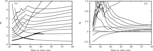
Modal diagram for envelope models having log L/L⊙ = 5.62, log Teff = 4.6 and solar chemical composition. Real (a) and imaginary (b) parts of the eigenfrequencies normalized by the global free fall time are given as a function of mass. Unstable modes are indicated by thick dots in (a) and negative imaginary parts in (b).
Real and imaginary parts of the eigenfrequencies normalized by the global free fall time are given in Figs 3(a) and (b), respectively. Thick dots in Fig. 3(a) and negative imaginary parts in Fig. 3(b) correspond to unstable modes. In general, the damping of modes increases with their frequency and order. Above a certain order (or sufficiently high frequency) which depends on stellar models, no unstable modes are found. Therefore, we have restricted our investigation to low-order modes. From Fig. 3 we deduce that models having masses below 53 M⊙ are unstable. The selected luminosity and effective temperature would correspond to an evolutionary track with an initial mass of 45 M⊙ (see Fig. 1). With decreasing mass the modal diagram becomes more complicated and exhibits a variety of mode crossings and interactions. Apart from oscillatory unstable modes, we also note the presence of a non-oscillatory (monotonically) unstable mode in models having masses below 30 M⊙. The existence of radial monotonically unstable modes with dynamical growth rates has been reported previously (e.g. Saio 2011; Yadav & Glatzel 2016). However, their physical origin and observational consequence is still an open question. In general, the strength of instabilities (growth rate) increases with the luminosity to mass ratio (see Fig. 3).
3.2 Evolutionary models
3.2.1 Models with initial masses of 100 and 70 M⊙
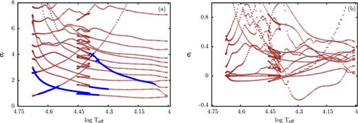
A modal diagram along the evolutionary track from the ZAMS to log Teff = 4.0 for an initial mass of 100 M⊙ (see Fig. 1) with the effective temperature as a parameter is shown in Fig. 4, where real (a) and imaginary (b) parts of the eigenfrequencies normalized by the global free fall time are displayed. All models considered are unstable with growth rates in the dynamical regime. Similar to Fig. 4, a modal diagram for an initial mass of 70 M⊙ is presented in Fig. 5. Compared to the 100 M⊙ mass models, the growth rates, the number of unstable modes and the range of instability have decreased slightly.
Modal diagram of envelope models along the evolutionary track from the ZAMS to an effective temperature of 10 000 K of a star with solar chemical composition and an initial mass of 100 M⊙. Real (a) and imaginary (b) parts of the eigenfrequencies normalized by the global free fall time are given as a function of effective temperature. Unstable modes are indicated by thick dots in (a) and negative imaginary parts in (b).
3.2.2 Models with initial masses of 45 and 30 M⊙
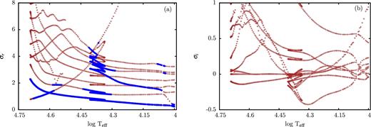
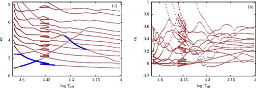
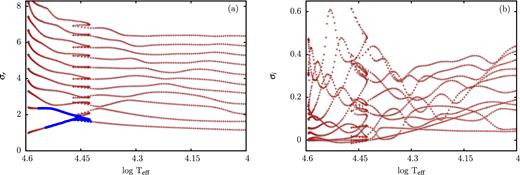
Modal diagrams along the evolutionary tracks with initial masses of 45 and 30 M⊙ are given in Figs 6 and 7, respectively. In both cases, models in the vicinity of ZAMS are linearly stable, which is in agreement with the previous study by Yadav & Glatzel (2017) on the stability of ZAMS models with solar chemical composition. This investigation has revealed that only models having masses above 58 M⊙ are unstable. For the 45 M⊙ track, instability sets in around log Teff = 4.62 and persists to log Teff = 4.40. Another strange mode is then unstable in the range between log Teff = 4.33 and 4.20. For the 30 M⊙ track, instability is found only in a narrow range of effective temperatures for 4.42 < log Teff < 4.56 (see Fig. 7).
3.2.3 Comparison with previous investigations
For low initial masses (see Fig. 7), modes are well separated and regularly spaced. If present, mode interactions occur via avoided crossings. With increasing initial mass (see Figs 4–6), mode interactions become more pronounced and the modal diagrams exhibit a bewildering complexity. Additional modes, some of them associated with instabilities in the dynamical range, appear in addition to the ordinary acoustic modes. In previous investigations (see e.g. Glatzel & Kiriakidis 1993b; Kiriakidis, Fricke & Glatzel 1993), they have been addressed as strange modes and strange mode instabilities, respectively. The number of unstable modes and the strength of the instabilities increase with the initial mass or the luminosity to mass ratio, respectively. Comparing our results with those of Kiriakidis et al. (1993), we find an overall agreement even quantitatively: the strange modes and associated instabilities fall into two groups related to the opacity bumps due to heavy elements and helium ionization, respectively. This becomes particularly obvious for the 45 M⊙ track, where the two groups are well separated and lead to a local maximum growth rate at log Teff ≈ 4.5 for the ‘heavy element strange modes’ and a local maximum growth rate at log Teff ≈ 4.3 for the ‘helium strange modes’. With respect to a recent publication by Daszyńska-Daszkiewicz et al. (2017) claiming the discovery of avoided crossings for radial main sequence stellar pulsations, we note that the phenomenon of mode coupling either through instability bands or avoided crossings is common in physics and astrophysics. For the spectrum of radial stellar pulsations, it was described by Gautschy & Glatzel (1990b), Glatzel & Kiriakidis (1993a), Glatzel et al. (1993) and Kiriakidis et al. (1993) for many types of stars including the ZAMS. For recent studies involving mode coupling phenomena in massive stars, we refer to Yadav & Glatzel (2016, 2017).
The boundary conditions for the perturbation equations at the photosphere are ambiguous. To account for this ambiguity, we have performed linear stability analyses for a variety of photospheric boundary conditions. Concerning the eigenfrequencies obtained for the models considered here the maximum relative differences for different boundary conditions amount to less than 15 per cent.
4 NON-LINEAR SIMULATIONS
In case of instability, the linear theory can predict neither the amplitude of an unstable perturbation nor the final fate of the system. In order to obtain the final fate of the unstable models which have been identified by linear stability analyses (see Section 3), instabilities have to be followed into the non-linear regime by numeral simulation. For the stellar models considered, instabilities may imply the following consequences:
Finite amplitude periodic or non-periodic pulsations, as found, e.g. for unstable models of massive stars by Grott, Chernigovski & Glatzel (2005) and Yadav & Glatzel (2017).
Eruption of the outer layers of a star, as noticed by Glatzel et al. (1999) in models of evolved massive stars and by Yadav & Glatzel (2016) in models of 55 Cygni. In these cases, the photospheric velocity exceeded the escape velocity in the course of the evolution of the instabilities.
Re-arrangement of the internal structure of the star, as pointed out by Yadav & Glatzel (2016) for one of the models for the supergiant 55 Cygni.
In order to determine the final fate of instabilities, we have followed them into the non-linear regime for selected unstable stellar models using the numerical scheme described by Grott et al. (2005). During pulsations, the acoustic energy fluxes and kinetic energies, being of interest here, are smaller than the gravitational and internal energies by several orders of magnitude. This requires the energy balance to be satisfied with an extremely high precision, which is achieved by an, with respect to energy, intrinsically conservative scheme. A consequence of the requirement of the conservativity is that the scheme has to be implicit with respect to time. The importance of conservativity in connection with the construction of numerical schemes and codes was repeatedly emphasized by Grott, Chernigovski & Glatzel (2003), Grott et al. (2005) and Glatzel & Chernigovski (2016). Using the procedure by Grott et al. (2005), for details we refer the reader to this publication, we can explicitly prove the energy balance to be satisfied intrinsically and thus show the results of our simulations to be reliable. Due to the occurrence of shock waves, artificial numerical viscosity has to be introduced to represent them. The choice of the artificial viscosity will be discussed in connection with the results in the subsequent sections.
Among various tests, the scheme used here had been applied during its development to classical Cepheids. Their instability caused by the κ-mechanism with imaginary parts of the eigenfrequencies corresponding to σi ∝ −10−2 is significantly weaker than the strange mode instabilities studied here. In these tests, the simulations have shown the instabilities to lead to finite amplitude pulsations with periods close to the linearly determined values and velocity amplitudes of the order of 10 km s−1. Likewise, we expect corresponding simulations for RR Lyrae models with stability properties similar to Cepheids to exhibit finite amplitude pulsations with periods close to the linearly obtained values. Non-linear studies for RR Lyrae models date back to Stellingwerf (1975). We note, however, that his approach prescribing a periodic behaviour is different from our study without any assumption on the evolution in the non-linear regime.
4.1 Models with distinct L/M values
The linear stability analysis of models having a fixed luminosity and effective temperature (log L/L⊙ = 5.62 and log Teff = 4.6) has revealed that models with masses below 53 M⊙ are unstable. To determine their final fate, we have followed the instabilities into the non-linear regime for selected unstable models with masses of 35, 30, 27 and 23 M⊙.
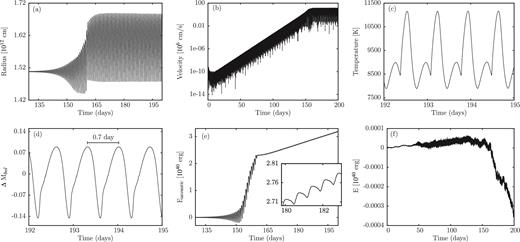
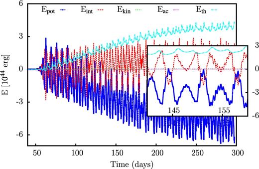
For a model with 35 M⊙, the results of the non-linear simulation are shown in Fig. 8. As a function of time, the stellar radius, velocity, density and temperature at the outermost grid point and the variation of the bolometric magnitude are given there. From the velocity, we deduce that the evolution of the instability starts from hydrostatic equilibrium with velocity perturbations of the order of 10−6 cm s−1 (the code picks up the correct unstable modes from numerical noise), undergoes the linear phase of exponential growth and saturates in the non-linear regime with a velocity amplitude of 190 km s−1. In this case, the final result of the instabilities are finite amplitude pulsations with a period of 8.4 h (0.35 d). A moderate inflation of the star is a consequence of non-linearities. Compared to the hydrostatic value, the mean radius is increased by approximately 10 per cent in the non-linear regime. Fig. 8 also contains the various terms involved in the energy balance, where the large hydrostatic values have been subtracted for a meaningful representation. Potential and internal energy with almost identical modulus have opposite sign and nearly cancel each other. They are by three and four orders of magnitude bigger than the kinetic and the time integrated acoustic energy, respectively, which are of main interest in our study. Due to the extreme differences in the order of magnitude of the various energies, the error in the energy balance is particularly important, since we are interested in the smallest energy terms. The error in the energy balance is in our normalization given by the sum of all energy terms which is shown in Fig. 8(i). It is smaller than the smallest term in the energy balance by at least four orders of magnitude proving the extreme accuracy of our simulation and the reliability of the results. The time integrated acoustic energy (see Fig. 8h) corresponds to the mechanical energy lost from the system by acoustic waves. During a pulsation cycle, there are phases of incoming and outgoing acoustic fluxes. As a consequence, the time integrated acoustic energy is a non-monotonic function. However, integrated over one cycle the outgoing energy exceeds the incoming energy and on average the time integrated acoustic energy increases with time. From Fig. 8(h), we obtain a well-defined mean slope of the integrated acoustic energy, which corresponds to a mean mechanical luminosity of the system. Assuming that this mean mechanical luminosity is responsible for mass-loss of the star, we can estimate the mass-loss rate by comparing it to the wind kinetic luminosity |$\frac{1}{2} \, \skew3\dot{M} \,v_{\infty } ^{2}$|, where |$\skew3\dot{M}$| and v∞ are the mass-loss rate and terminal wind velocity, respectively (see also Grott et al. 2005; Yadav & Glatzel 2016, 2017). The terminal wind velocity is estimated by the escape velocity. Thus, we obtain from the mean slope of the time integrated acoustic energy (Fig. 8h), a mass-loss rate of 3.9 × 10⁻⁹ M⊙ yr−1 for the 35 M⊙ model.
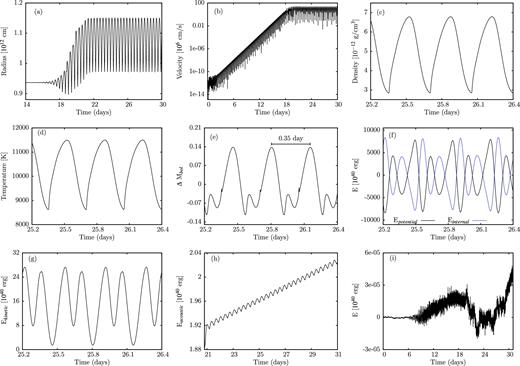
Evolution of the instability into the non-linear regime and finite amplitude pulsations for a model having M = 35 M⊙, log L/L⊙ = 5.62 and Teff = 40 000 K. As a function of time, the stellar radius, velocity, density and temperature at the outermost grid point are shown in (a)–(d), respectively, the variation of the bolometric magnitude is given in (e). From the velocity diagram (b), we deduce that the evolution of the instability starts from hydrostatic equilibrium with velocity perturbations of the order of 10−6 cm s−1, undergoes the linear phase of exponential growth and saturates in the non-linear regime with a velocity amplitude of 190 km s−1. Compared to the hydrostatic value, the mean radius is increased by approximately 10 per cent in the non-linear regime. The various terms appearing in the energy balance are shown in (f)–(h), where the hydrostatic values have been subtracted. Potential and internal energy with almost identical modulus have opposite sign. They are by three and four orders of magnitude bigger than the kinetic and the time integrated acoustic energy, respectively. The sum of all energy terms is given in (i) indicating the error in the energy balance. Note that this error is smaller than the smallest term in the energy balance by at least four orders of magnitude.
The time integrated acoustic energy is made up of the fluxes of the kinetic and compression energies contained in a sequence of hypersonic shock waves with associated overdense shells leaving the outer boundary of the integration domain. In the atmosphere of the star, where radiation transport needs to be considered in detail being beyond the scope of this study, the shock wave together with its overdense shell is then expected to undergo a snowplow phase sweeping up the atmosphere material and transferring its momentum to the expanding shell which leaves the system, thus implying mass-loss. Although this process is certainly not stationary, it provides the motivation to estimate the mass-loss rate by comparing the mean acoustic luminosity to the kinetic luminosity of a stationary wind with a terminal wind velocity of the order of the escape speed.
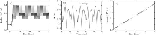
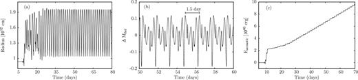
The instabilities considered become stronger with increasing luminosity to mass ratios (see Fig. 3b). Therefore, we expect their final result to become more pronounced, i.e. the amplitudes of the finite amplitude pulsations to increase with L/M. The results for models having masses of 30 and 27 M⊙ are displayed in Figs 9 and 10, respectively, similar to their counterpart in Fig. 8 for the 35 M⊙ model. The periods and velocity amplitudes of the finite amplitude pulsations amount to 0.94 and 1.5 d and 196 and 281 km s−1 for the 30 and 27 M⊙ models, respectively. As expected, also the effect of inflation of the mean radius becomes more pronounced with increasing L/M or strength of the instability, respectively. The increase of the pulsation periods with L/M can then be understood by the period density relation, since both lower masses and inflated radii imply lower densities. The mean mechanical luminosity derived from the mean slope of the time integrated acoustic energy in Figs 9(c) and 10(c) provides an estimate for the mass-loss rates of the 30 and 27 M⊙ models of 8.9 × 10⁻⁹ and 7.0 × 10⁻⁸ M⊙ yr−1, respectively. Again, the increase of the mass-loss rate with L/M supports the idea of a direct relation between the strength of the instability and mass-loss. Errors in the energy balance are similar to those shown for the 35 M⊙ model.
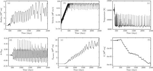
The 23 M⊙ model having the highest L/M ratio of the models selected suffers from the most violent instabilities found. The results of the simulation of the evolution of these instabilities into the non-linear regime are presented in Fig. 11. The velocity at the outermost grid point shows that the instability starts from hydrostatic equilibrium with perturbations of the order of 10−6 cm s−1 and saturates after the linear phase of exponential growth in the non-linear regime with a maximum velocity of 315 km s−1. Associated with these high velocities is an inflation of the stellar radius by a factor of approximately 5. As a consequence, the temperature at the outermost grid point drops to approximately 5000 K. For even lower temperatures, opacities were not available and we had to stop the simulation. The maximum velocity of 315 km s−1 has to be compared with the escape velocity of 390 km s−1. Even if the evolution could not be followed further, we may take this result as an indication for direct mass-loss. Again, errors in the energy balance are similar to those shown for the 35 M⊙ model.
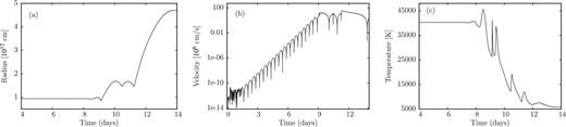
Same as Fig. 8 but for M = 23 M⊙. For this model the radius is inflated substantially which is associated with a strong temperature decrease. Due to the latter, the simulation had to be stopped because opacity data were not available for low temperatures.
4.2 Evolutionary models
For selected models on the evolutionary tracks shown in Fig. 1, which have been determined to be unstable by the linear analysis in Section 3, we have performed numerical simulations of the evolution of the instabilities into the non-linear regime to determine the final fate of the corresponding objects.
4.2.1 Models having log Teff = 4.6
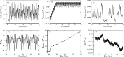
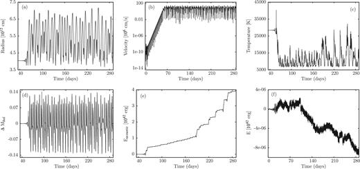
For an effective temperature of log Teff = 4.6, only models on the evolutionary tracks for initial masses of 100 and 70 M⊙ are unstable. The results of our numerical simulations of the evolution of these unstable models are displayed in Figs 12 and 13, respectively. In these figures, the stellar radius (a), velocity (b) and temperature (c) at the outermost grid point, the variation of the bolometric magnitude (d), the time integrated acoustic energy (e) and the error in the energy balance (f) are given as a function of time. For both models, the final fate appears to be finite amplitude pulsation where the mean radius is slightly inflated and velocity amplitudes of 255 and 262 km s−1 (corresponding to ≈30 per cent of the escape velocity) are attained. Similar to the previously discussed models, the evolution starts from hydrostatic equilibrium with velocity perturbations of the order of 10−6 cm s−1 on the numerical noise level, goes through the linear phase of exponential growth and finally saturates in the non-linear regime. For the model with an initial mass of 100 M⊙ in the non-linear regime, a strictly periodic pattern with a period of 3.2 d can be identified, whereas for the 70 M⊙ model the pattern is no longer strictly periodic, although at least one dominant period may be deduced from the variation of the bolometric magnitude.
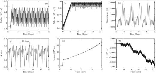
Evolution of the instability into the non-linear regime and finite amplitude pulsations for a model having log Teff = 4.6 on the evolutionary track of a star with an initial mass of 100 M⊙ (see Fig. 1). As a function of time, the stellar radius, velocity and temperature at the outermost grid point are shown in (a)–(c), respectively, the variation of the bolometric magnitude is given in (d). The velocity amplitude reaches 255 km s−1 in the non-linear regime. The time integrated acoustic energy (being the smallest term in the energy balance) and the error of the energy balance are displayed in (e) and (f), respectively.
Same as Fig. 12 but for a star with an effective temperature of log Teff = 4.6 and an initial mass of 70 M⊙. The finite amplitude pulsation does not exhibit a strictly periodic pattern. The velocity amplitude reaches 262 km s−1 in the non-linear regime.
As in the previous section, the mass-loss rate is estimated by comparing the mean slope of the time integrated acoustic energy to the kinetic wind luminosity. The mean slope of the time integrated acoustic energy is well defined for the 70 M⊙ model (see Fig. 13) allowing for a unique determination of a mass-loss rate, whereas the mean slope varies for the 100 M⊙ model and only a range of mass-loss rates together with a maximum mass-loss rate can be estimated. Accordingly, we obtain a mass-loss rate of 2.1 × 10⁻⁷ M⊙ yr−1 for the 70 M⊙ model from Fig. 13 and a maximum mass-loss rate of 1.9 × 10⁻⁷ M⊙ yr−1 for the 100 M⊙ model from Fig. 12. From the run of the time integrated acoustic energy (see Fig. 12), we suspect that the latter might be even higher if we would have followed the evolution for more than 100 d. The errors in the energy balance given in Figs 12(f) and 13(f) are smaller than the smallest term in the energy balance (the time integrated acoustic energy) by more than four orders of magnitude. The other terms in the energy balance exhibit similar orders of magnitude as discussed for the models in the previous section.
4.2.2 Models having log Teff = 4.45
For the effective temperature log Teff = 4.45, all stellar models on the evolutionary tracks for the initial masses of 100, 70, 45 and 30 M⊙ are linearly unstable. Results of the simulations of the evolution of the instabilities into the non-linear regime are shown in Figs 14–17, respectively. Essentially the discussion of the results given for the models having log Teff = 4.6 also holds for those considered here. The velocity amplitudes attain values between 130 and 215 km s−1. Except for the 100 M⊙ model, where the finite amplitude pulsation is not strictly periodic and a pulsation period cannot be defined, the non-linear pulsation periods lie in the range between 0.7 and 2.37 d. From the mean slope of the time integrated acoustic energy, we obtain mass-loss rates of 4.5 × 10⁻⁸, 4.2 × 10⁻⁸ and 1.7 × 10⁻⁸ M⊙ yr−1 for models corresponding to initial masses of 70, 45 and 30 M⊙, respectively. For the 100 M⊙ model, we estimate a maximum mass-loss rate of 1.7 × 10⁻⁶ M⊙ yr−1.
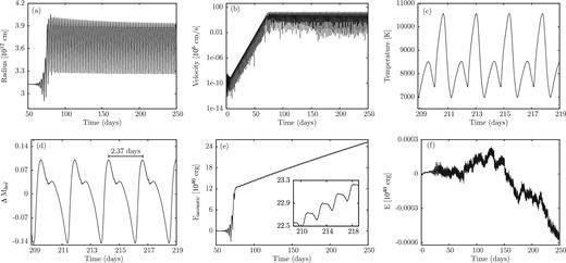
Same as Fig. 12 but for a star with log Teff = 4.45 and an initial mass of 70 M⊙. The velocity amplitude reaches 131 km s−1 in the non-linear regime.
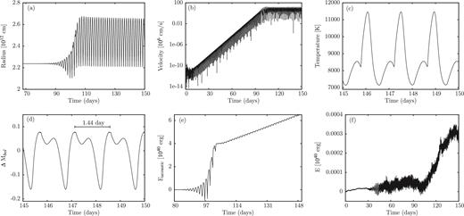
Same as Fig. 12 but for a star with log Teff = 4.45 and an initial mass of 45 M⊙. The velocity amplitude reaches 139 km s−1 in the non-linear regime.
Same as Fig. 12 but for a star with log Teff = 4.45 and an initial mass of 30 M⊙. The velocity amplitude reaches 130 km s−1 in the non-linear regime.
4.2.3 Models having log Teff = 4.15
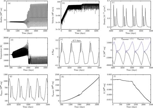
For the effective temperature log Teff = 4.15, only models having high initial masses of 100 and 70 M⊙ are linearly unstable. Results of the simulations of the evolution of the instabilities into the non-linear regime are shown in Figs 18 and 19, respectively. Again, essentially the discussion of the results given for the models having log Teff = 4.6 also holds for those considered here. The velocity amplitudes attain values of 131 and 102 km s−1. In the 100 M⊙ model, the finite amplitude pulsation is not strictly periodic and a pulsation period cannot be defined, for the 70 M⊙ model a non-linear pulsation period of 47.7 d is obtained. From the mean slope of the time integrated acoustic energy, we obtain mass-loss rates of 2.1 × 10⁻⁶ and 2.9 × 10⁻⁶ M⊙ yr−1 for models corresponding to initial masses of 100 and 70 M⊙, respectively. We note that for the 100 M⊙ model, the mean slope of the time integrated acoustic energy is less well defined than for other models discussed here. Moreover, this model exhibits a considerable inflation of the radius. In Fig. 19, we have added plots of the potential, internal and kinetic energy terms as a function of time for the 70 M⊙ model, since in this case they are higher by one order of magnitude compared to the values obtained for the 35 M⊙ model discussed in Fig. 8.
4.3 Long-term simulations for the determination of the mean acoustic luminosity
For some unstable models, the mean slope of the time integrated acoustic energy does not yet reach a constant value even for sufficiently advanced times in the non-linear regime, where the finite amplitude pulsations have reached a quasi-stationary state otherwise (see Sections 4.2.1 and 4.2.3). For the evolutionary model having an initial mass of 100 M⊙ and log Teff = 4.6 (see also Fig. 12 and its discussion), we have therefore performed long-term simulations covering more than 200 pulsation periods. The results, i.e. the time integrated acoustic and thermal energies as a function of time are shown in Fig. 20. After 500 d, the mean slope both of the time integrated acoustic and thermal energy appears to reach a constant value. For the time integrated acoustic energy, it corresponds to a mass-loss rate of 1.8 × 10⁻⁵ M⊙ yr−1. For a 100 M⊙ star with a typical lifetime of around 106 yr, a mass-loss rate of this order can affect its evolution. From Fig. 20, we deduce that the mean slopes of the time integrated acoustic and thermal energies have approximately the same modulus but opposite sign. Accordingly, the associated acoustic and thermal luminosities (the latter being negative) cancel. This is interpreted as a transformation of thermal flux into acoustic flux on the basis of the pulsations acting as a Carnot type heat engine. Note that the total thermal luminosity being the sum of the stationary thermal luminosity and the variable contribution are always positive. In our discussions, we have always subtracted stationary contributions from the hydrostatic background model. Similar to the model having an initial mass of 100 M⊙ and log Teff = 4.6, we have performed a long-term simulation for the model having 100 M⊙ and log Teff = 4.45 (see Fig. 14). In this case, the mass-loss rate is found to increase from 1.7 × 10⁻⁶ to 1.4 × 10⁻⁴ M⊙ yr−1.
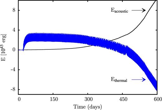
Time integrated acoustic and thermal energies as a function of time for an evolutionary model having an initial mass of 100 M⊙ and log Teff = 4.6.
4.4 Role of artificial viscosity in non-linear regime
The instabilities identified here have the character of sound wave. In the course of evolution, any sound wave will steepen and finally form a shock wave. Thus, the appearance of shock waves is expected, when the instabilities are followed into the non-linear regime. Any numerical technique faces difficulties in representing discontinuous functions such as shock waves. An approach to handle shock waves without violating the requirement of the conservativity of the numerical scheme consists of the introduction of artificial viscosity (see Von Neumann & Richtmyer 1950). Meanwhile, many forms of the artificial viscosity have been proposed (see e.g. Tscharnuter & Winkler 1979). In this study, we adopt the artificial viscosity as given by Grott et al. (2005). Among others, Noh (1987) has pointed out that the artificial viscosity can imply artefacts and may lead to erroneous numerical results. Therefore, the influence of the artificial viscosity on the numerical solutions needs to be studied. In particular, the dependence on the viscosity parameter ν0 introduced by Grott et al. (2005) has to be investigated. Its appropriate choice is expected to depend on the stellar model considered.
In the linear regime of exponential growth of the instabilities, the influence of the artificial viscosity is negligible since the compression rates defining the artificial viscosity remain sufficiently small. In any case, artificial viscosity is important and implies consequences only in the vicinity of shocks. Numerical oscillations of, e.g. the density stratification in the vicinity of a shock (Gibbs phenomenon) indicate that the numerical viscosity chosen is too small. In general, the viscosity parameter is chosen as small as possible but high enough such that these oscillations are marginally suppressed. A value of ν0 = 10 turned out to be appropriate for many stellar models. The influence of ν0 on the results is illustrated in Fig. 21 for an evolutionary model with log Teff = 4.3 and an initial mass of 70 M⊙. From Fig. 21, we deduce that radius, velocity, variations of the bolometric magnitude and the density stratification even in the vicinity of a shock are not substantially affected by varying the artificial viscosity even by two orders of magnitude. Moreover, a value of ν0 = 10 is apparently sufficient to suppress the Gibbs phenomenon. The latter seems to be more pronounced in the variation of the bolometric magnitude when considering it on a smaller scale. In the most extreme case, i.e. at the outermost grid point, the variation of the temperature in the passing shock is considerably reduced by artificial viscosity. Thus, conclusions concerning temperature variations should be drawn with caution. Substantially, affected by the artificial viscosity is the mean slope of the time integrated acoustic energy used for the estimate of the mass-loss rate. It increases with decreasing ν0 implying an (expected) enhanced redistribution of mechanical into thermal energy with increasing artificial viscosity. Therefore, the mass-loss rates based on the mean slope of the time integrated acoustic energy derived here should be considered as lower limits to the actual pulsationally driven mass-loss rates. From the mean slope of the time integrated acoustic energy (Fig. 21d), we obtain for the viscosity parameter ν0 = 5, 10 and 100 a mass-loss rate of 5.1 × 10⁻⁷, 3.0 × 10⁻⁷ and 1.1 × 10⁻⁷ M⊙ yr−1, respectively.
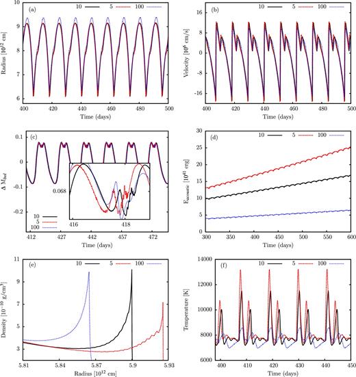
The influence of the artificial viscosity parameter (ν0 = 5, 10, 100) on the finite amplitude pulsations of an evolutionary model with log Teff = 4.3 and an initial mass of 70 M⊙. Radius, velocity at the outermost grid point, the variation of the bolometric magnitude, the time integrated acoustic energy and the temperature at the outermost grid point are given as a function of time in (a), (b), (c), (d) and (f), respectively, the density stratification is given in (e) as a function of radius at comparable instances of time.
4.5 Linearly stable models
For unstable models, we have seen that the velocity amplitude grows from numerical noise (10−4 cm s−1) without any external perturbation and saturates in the non-linear regime with maximum amplitudes of the order of 100 km s−1. To test and validate the code, we have also performed simulations of the evolution of linearly stable models (see also Yadav & Glatzel 2017). In this case, the code should not pick up any instability and, as a result, the velocity amplitude should always remain on the numeral noise level of the scheme. The latter is controlled by the prescribed relaxation accuracy of the initial hydrostatic model. As an example, velocities at the outermost grid point are given as a function of time in Fig. 22 for two linearly stable models. For both models, the velocity amplitudes remain on the numerical noise level which proofs that the final results of the simulations are due to physical instabilities (if present) rather than to numerical instabilities and artefacts.
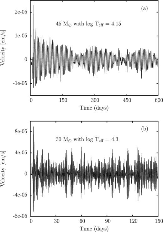
The velocity at the outermost grid point as a function of time for two linearly stable evolutionary models with an effective temperature of log Teff = 4.15 and an initial mass of 45 M⊙ (a), and an effective temperature of log Teff = 4.3 and an initial mass of 30 M⊙ (b). The velocity remains on the numerical noise level.
5 DISCUSSION AND CONCLUSIONS
The linear instability of massive stars in the upper domain of the HR diagram has been known now for more than 20 yr (see e.g. Glatzel & Kiriakidis 1993a; Kiriakidis et al. 1993). Instabilities with growth rates in the dynamical range are associated with the appearance of strange modes and rely on a non-classical mechanism described by Glatzel (1994). They fall into three groups related to the three opacity maxima due to the contribution of heavy elements, helium and hydrogen ionization, respectively. In the first part of this paper, we have redone the linear stability analysis of massive stars on the basis of the latest available opacity and equation of state tables. As a result, the previous investigations have been confirmed qualitatively. In particular, for the range of models considered, the maxima in the growth rates related to opacity maxima due to heavy elements and the first helium ionization have been established. Contrary to the linear stability analysis, non-linear investigations concerning the final result of the instabilities are rare (see e.g. Glatzel et al. 1999; Grott et al. 2005; Yadav & Glatzel 2016, 2017). In particular, a systematic non-linear study of massive stars in the upper domain of the HRD is not yet available. Accordingly, the latter was the motivation and main subject of this paper.
The lack of numerical studies of the evolution of stellar instabilities into the non-linear regime is due to extreme numerical difficulties caused by huge differences in the order of magnitude of the various forms of the energy involved in a stellar pulsation. Typically gravitational and internal energies exceed the kinetic energy of interest by four orders of magnitude. Thus, for meaningful results, the numerical scheme has to represent the energy balance correctly with a relative accuracy better than 10−5. This condition requires the numerical scheme to be intrinsically fully conservative with respect to energy. For non-conservative schemes, numerical errors lead to kinetic energies comparable to gravitational and internal energies and thus to erroneously high-velocity amplitudes and mass-loss (see e.g. Appenzeller 1970; Moriya & Langer 2015). For this study, we have adopted the fully conservative scheme described by Grott et al. (2005).
In any case, the result of the instabilities considered are finite amplitude pulsations where the velocity amplitudes (of the order of 100 km s−1) attain a significant fraction of the escape velocity. Caused by sequences of shock waves the envelope becomes considerably inflated in the non-linear regime for many models. As a consequence, the final finite amplitude pulsation period is bigger than the linearly determined period of the unstable mode. Therefore, for a comparison with observed pulsation periods, the finite amplitude pulsation periods should be used rather than periods determined by a linear stability analysis. The inflation of the envelope is also associated with a decrease in temperature which occasionally was so strong that for the temperatures reached, opacity data were no longer available. Unfortunately, in these cases we had to stop the simulation. In the non-linear regime, the mean slope of the time integrated acoustic energy was always positive indicating an outward directed mechanical acoustic luminosity. Comparing this acoustic luminosity with a kinetic wind luminosity, we were able to estimate pulsationally driven mass-loss rates. Depending on the stellar model mass-loss rates in the range between 10−9 and 10−4 M⊙ yr−1 have been derived.
Compared to unstable ZAMS models, the pulsation periods of the evolved models considered here having substantially larger radii are significantly longer as a consequence of the period density relation. Similarly, the maximum mass-loss rate of 10−4 M⊙ yr−1 for the evolved models compared to 10−7 M⊙ yr−1 for ZAMS objects is due to larger radii and less bound envelopes, where the velocity amplitudes are of the order of 100 km s−1 in both cases. For the extended evolved models, the velocity amplitudes amount to a larger fraction of the escape speed.
For the representation of shock waves occurring in the course of the evolution of the instabilities, artificial viscosity had to be introduced. Whether and how it influences the solution had to be studied. Quantities as pulsation periods, velocities (including amplitudes), bolometric magnitudes and radius variations are almost unaffected even for a large variation of the viscosity parameter. However, the time integrated acoustic energy and its mean slope sensitively depends on the artificial viscosity, where the mean slope increases with decreasing artificial viscosity. Thus, the estimated mass-loss rates have to be regarded as lower limits to the actual values.
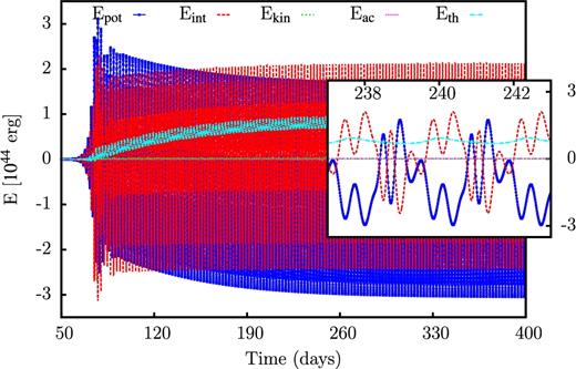
The dependence on the stellar model of the run of the various forms of the energy is noteworthy. As an example, in Figs 23– 25 the energies are given as a function of time for three evolutionary models with log Teff = 4.45 having initial masses of 30, 70 and 100 M⊙, respectively. In any case, the relative error in the energy balance lies below 10−7 and the time integrated acoustic energy as well as the kinetic energy is much smaller than the other terms. For the 30 M⊙ model, even the time integrated thermal flux is negligible compared to the internal and the gravitational potential energy (see Fig. 23). The latter form a symmetric pair and almost cancel each other. For the 70 M⊙ model, this symmetry is lifted, since the time integrated thermal flux becomes comparable to the internal and the potential energies. Now, the sum of the time integrated thermal flux, the potential and the internal energy approximately cancel (see Fig. 24). This situation becomes even more pronounced for the 100 M⊙ model, where the time integrated thermal flux even exceeds the internal energy (see Fig. 25).
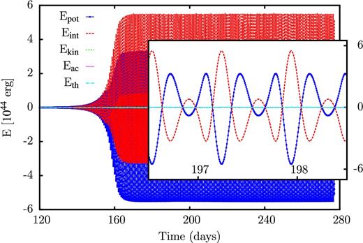
Potential, internal, kinetic, time integrated acoustic and time integrated thermal energy as a function of time for an evolutionary model with log Teff = 4.45 having an initial mass of 30 M⊙.
The importance of the time integrated thermal flux has been realized for stellar models, for which we were able to perform long-term simulations of the evolution of the finite amplitude pulsations. In these cases, the mean slope of the time integrated acoustic energy (and the associated mass-loss rate) was found to increase considerably in the course of long-term evolution. Simultaneously, the mean slopes of the time integrated acoustic and (significant) thermal energies have approximately the same modulus but opposite sign. This means that acoustic and thermal luminosities cancel, which is interpreted as a transformation of thermal flux into acoustic flux. The observation that in the course of long-term evolution, the mean acoustic luminosity (and with it the mass-loss rate) may be supported by and at the cost of the thermal luminosity, thus being considerably enhanced, indicates that the mass-loss rates estimated here have to be regarded as lower limits, since long-term simulations could be performed only for selected models.
This study was restricted to the consideration of spherically symmetric perturbations and pulsations. Both from observations (Kraus et al. 2015) and linear non-radial stability analyses (Glatzel & Mehren 1996), we know that the models considered here do also suffer from non-radial strange mode instabilities. Therefore, an investigation of the evolution of non-radial instabilities into the non-linear regime is necessary. However, corresponding numerical tools satisfying the conservativity requirement are not yet available. Thus, the development of appropriate schemes is highly recommended.
Acknowledgements
APY gratefully acknowledges financial support by a SmartLink - Erasmus Mundus post-doc fellowship.
REFERENCES
