


Abstract
We study a sample of 23 Type II plateau supernovae (SNe II-P), all observed with the same set of instruments. Analysis of their photometric evolution confirms that their typical plateau duration is 100 d with little scatter, showing a tendency to get shorter for more energetic SNe. We examine the claimed correlation between the luminosity and the rise time from explosion to plateau. We analyse their spectra, measuring typical ejecta velocities, and confirm that they follow a well-behaved power-law decline. We find indications of high-velocity material in the spectra of six of our SNe. We test different dust-extinction correction methods by asking the following – does the uniformity of the sample increase after the application of a given method? A reasonably behaved underlying distribution should become tighter after correction. No method we tested made a significant improvement.
1 INTRODUCTION
Stars more massive than ∼8 M⊙ end their lives as core-collapse supernovae (CC-SNe). This is based on multiple lines of evidence, from their locations, in or near regions of star formation, to multiple progenitor identifications (see Smartt 2009 for a review). The explosions of stars that have kept a large hydrogen envelope until their demise are observationally defined as Type II SNe, based on the presence of broad hydrogen lines in their spectra with line widths of several thousand km s−1. The lines typically have P-Cygni profiles, formed by the expanding hydrogen-rich ejecta.
Type II SNe are a diverse class, with a large range of observed luminosities, light-curve shapes, and spectroscopic features. These have been historically used to further subclassify these events. The optical light-curve shape has been used to separate those that decline linearly with time (II-L) from those that show a pronounced plateau (II-P; Barbon, Ciatti & Rosino 1979). Later, two more classes were defined spectroscopically, SNe IIn that have relatively narrow hydrogen emission lines attributed to interaction of the ejecta with circumstellar (CS) matter (Schlegel 1990) and SNe IIb that are spectroscopically intermediate between SNe II and SNe Ib (see Filippenko 1997 for a review). SNe Ib are interpreted as arising from stars stripped of their envelope, as indicated by their helium dominated, hydrogen-free spectra. SNe IIb early-time spectra evolve from hydrogen-rich to SN Ib-like spectra (Filippenko 1988).
Individual SNe II-P have been well studied in the past thanks to their proximity. Examples include SN 1999em (e.g. Baron et al. 2000; Leonard et al. 2002a; Dessart & Hillier 2006) and SN 1999gi (Leonard et al. 2002b). Both objects have progenitor mass estimates – a very tight restriction on the upper mass of the SN 1999em progenitor was derived by Smartt et al. (2009), who found 15 M⊙, and for SN 1999gi Smartt et al. (2001) report an upper limit of 9|$^{+3}_{-2}$| M⊙. Another example of a nearby, well-studied event is SN 2005cs (e.g. Pastorello et al. 2009); it had a low-luminosity and a moderate-mass progenitor.
Until recently, there were very few studies of samples of SNe II-P. Hamuy & Pinto (2002) and Hamuy (2003) analysed a sample of ∼20 SNe II-P, and found relations between plateau luminosity, ejecta velocities, and nickel abundances, as well as a useful luminosity–velocity relation which allows for distance measurements. This is an empirical application of the expanding photosphere method (Kirshner & Kwan 1974; Eastman, Schmidt & Kirshner 1996; Dessart & Hillier 2005b; Dessart et al. 2008; Jones et al. 2009). This method and its potential for cosmological distance measurements were further studied by Nugent et al. (2006), Poznanski et al. (2009), D'Andrea et al. (2010), Poznanski, Nugent & Filippenko (2010), and Olivares et al. (2010). Maguire et al. (2010a) examined its extension into the infrared. Arcavi et al. (2012) analysed a small sample of SNe II-P, contrasting them with other SNe II, and found that while they differ wildly in luminosity, they seem to have similar plateau durations, all near 100 d.
However, in the past few months several new studies have seen light. Spiro et al. (2014) study low-luminosity events and find that they constitute the tail of the distribution of SNe II-P (as we also show below). While this paper was in final editing stages, Anderson et al. (2014b) published an analysis of Type II SN photometry. They present a sample of more than 100 V-band light curves. Their results are consistent with some of our photometric findings, namely that these SNe seem to form a continuous class, with a range of luminosities, with a correlation between plateau duration and brightness. However, they consider a larger range of SNe, including objects that we would classify as II-L and analyse separately in a companion paper (Faran et al. 2014). Lastly, after our paper was submitted, Sanders et al. (2014) published their analysis of a sample of 76 light curves of Type II-P SNe, with similar results.
Here we present a sample of 23 SNe II-P, some which have been studied before (Hamuy et al. 2001; Elmhamdi et al. 2003; Hendry et al. 2005; Pozzo et al. 2006; Sahu et al. 2006; Tsvetkov et al. 2006; Misra et al. 2007; Jones et al. 2009; Maguire et al. 2010b; Olivares et al. 2010; Arcavi et al. 2012; Spiro et al. 2014), but many have not. All SNe were observed by the Lick Observatory SN Search (LOSS; Filippenko et al. 2001), have high-cadence photometry in three to four bands, and between few and tens of optical spectra. This results in a data set with 1574 photometric points and 152 spectra. We further use this sample to examine methods for dust-extinction correction.1
2 OBSERVATIONS
Imaging was obtained with the 0.76 m Katzman Automatic Imaging Telescope (KAIT), the SN search engine of LOSS. The sample was compiled from events for which precise photometry could be obtained – that is, for which template images were obtained after the SN had faded. Since the focus on the study is SNe II-P, we only include objects with a pronounced plateau in the light curve, removing SNe II-L, IIb, IIn, and peculiar SNe, such as SN 2000cb, a SN 1987A-like object (Kleiser et al. 2011). The distinction between II-P and II-L events will be defined by Faran et al. (2014).
KAIT images of the SNe were reduced as described by Poznanski et al. (2009), Ganeshalingam et al. (2010), and Silverman et al. (2012). Briefly, after standard image reduction, image subtraction was performed, using galaxy templates obtained with KAIT on photometric nights, at least a few months after the SN had faded beyond detection. Photometry was obtained using differential point spread function fitting using the daophot package in iraf, in order to measure the SN flux relative to local standards in the field. Calibrations were obtained on photometric nights using both the KAIT and the 1 m Nickel telescope at Lick Observatory. We correct the magnitudes for Galactic extinction using the maps of Schlegel, Finkbeiner & Davis (1998).
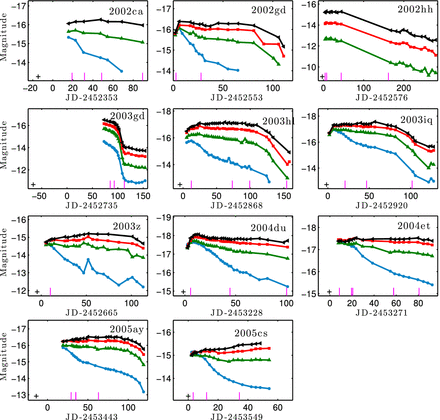
In Figs 1 and 2, we show the BVRI light curves of our 23 SNe, marking the epochs at which spectra were taken. The light curves are typically better sampled than the time-scales for brightness change, so it is safe to interpolate the photometry when needed. Information on the SNe is presented in Table 1. The explosion day is set as the mid-point between the first detection and the last non-detection, and the uncertainty is conservatively set as half the difference. There are three objects with weak constraints. For SN 2002gd, a rough estimate for the explosion day can be obtained by comparing the epoch of peak brightness to SNe with similar light curves. The photometry of SN 1999D and SN 2001hg does not even allow that. These objects are naturally excluded from analyses where time reference is required.
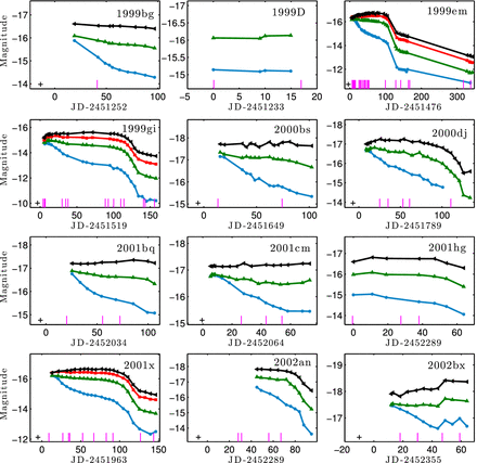
Light curves of the 23 SNe in our sample. B (blue circles), V (green triangles), R (red squares), and I (black side triangles). Magenta ticks mark the epochs at which spectra were obtained. The black crosses denote the last non-detections. SNe 1999D and 2001hg are plotted relative to the first photometric point. Continued in Fig. 2.
SN sample.
| SN name | zhost | μa | Explosion MJD | E(B − V)MWc |
|---|---|---|---|---|
| 1999bg | 0.0043 | 31.83 | 51251 (14) | 0.0184 |
| 1999D | 0.0104 | 33.17b | – | 0.0166 |
| 1999em | 0.0024 | 29.95 | 51476 (4) | 0.0400 |
| 1999gi | 0.0020 | 29.55 | 51518 (4) | 0.0166 |
| 2000bs | 0.0280 | 35.30b | 51648 (6) | 0.0317 |
| 2000dj | 0.0154 | 34.19 | 51788 (7) | 0.0734 |
| 2001bq | 0.0087 | 32.78b | 52034 (6) | 0.0441 |
| 2001cm | 0.0114 | 33.48 | 52063 (1) | 0.0124 |
| 2001hg | 0.0086 | 33.00 | – | 0.0351 |
| 2001X | 0.0049 | 31.37 | 51963 (5) | 0.0401 |
| 2002an | 0.0129 | 33.85 | 52288 (8) | 0.0348 |
| 2002bx | 0.0075 | 34.42 | 52354 (10) | 0.0118 |
| 2002ca | 0.0109 | 33.26b | 52353 (15) | 0.0242 |
| 2002gd | 0.0089 | 33.07 | 52552 (?) | 0.0676 |
| 2002hh | 0.0001 | 28.87 | 52576 (3) | 0.3413 |
| 2003gd | 0.0022 | 29.66 | 52735 (67) | 0.0682 |
| 2003hl | 0.0082 | 32.68 | 52867 (5) | 0.0734 |
| 2003iq | 0.0082 | 32.68 | 52920 (2) | 0.0725 |
| 2003Z | 0.0043 | 31.77 | 52664 (5) | 0.0384 |
| 2004du | 0.0168 | 34.40 | 53228 (2) | 0.0947 |
| 2004et | 0.0001 | 28.87 | 53271 (1) | 0.3415 |
| 2005ay | 0.0027 | 31.15 | 53442 (14) | 0.0214 |
| 2005cs | 0.0015 | 29.51 | 53549 (0.5) | 0.0347 |
aDistance modulus (mag) from NED, unless noted otherwise.
bRedshift-based distance.
cMag, assuming RV = 3.1.
Distance measurements are collected from NED2 and averaged, using only distances based on the Tully–Fisher method, Cepheids, and SNe Ia. When the distance is ambiguous or unknown, we derive the distance to the SN using Hubble's law and the redshift, using a Hubble constant of H0 = 73 km s−1 Mpc−1, assuming an uncertainty of 10 per cent. All of the objects in our sample are at low redshifts with z < 0.03.
We obtained optical spectra with the Kast double spectrograph (Miller & Stone 1993) mounted on the Lick Observatory 3 m Shane telescope, the Low Resolution Imaging Spectrometer (LRIS; Oke et al. 1995) on the 10 m Keck-I telescope, the Stover spectrograph mounted on the 1 m Nickel telescope, and the Deep Imaging Multi-Object Spectrograph (Faber et al. 2003) on the 10 m Keck-II telescope. Reduction details are given by Poznanski et al. (2009) and Li et al. (2001).
Partial photometric and spectroscopic data are shown in Tables 2 and 3. Complete data are available in the electronic version.
Partial photometric data of the KAIT sample.
| SN name | MJD | Agea | B(σB) | V(σV) | R(σR) | I(σI) |
|---|---|---|---|---|---|---|
| 1999em | 51481.39 | 5.4 | 13.704(0.010) | 13.782(0.010) | 13.621(0.010) | 13.640(0.035) |
| 1999em | 51482.43 | 6.5 | 13.677(0.010) | 13.718(0.010) | 13.577(0.010) | 13.578(0.036) |
| 1999em | 51483.43 | 7.5 | 13.675(0.010) | 13.713(0.010) | 13.539(0.010) | 13.568(0.031) |
| ⋅⋅⋅ | ⋅⋅⋅ | ⋅⋅⋅ | ⋅⋅⋅ | ⋅⋅⋅ | ⋅⋅⋅ | |
| 1999gi | 51523.52 | 5.4 | – | 14.736(0.020) | 14.552(0.011) | 14.381(0.020) |
| 1999gi | 51524.56 | 6.4 | 14.861(0.034) | 14.744(0.033) | 14.481(0.012) | 14.286(0.013) |
| 1999gi | 51527.48 | 9.3 | 14.763(0.034) | 14.614(0.013) | 14.299(0.010) | 14.116(0.010) |
| ⋅⋅⋅ | ⋅⋅⋅ | ⋅⋅⋅ | ⋅⋅⋅ | ⋅⋅⋅ | ⋅⋅⋅ | |
| 2001X | 51975.55 | 12.9 | 15.161(0.014) | 15.169(0.010) | 14.973(0.012) | 14.974(0.032) |
| 2001X | 51983.52 | 20.9 | 15.371(0.012) | 15.178(0.010) | 14.915(0.011) | 14.875(0.018) |
| 2001X | 51988.50 | 25.8 | 15.681(0.065) | 15.257(0.072) | – | – |
| ⋅⋅⋅ | ⋅⋅⋅ | ⋅⋅⋅ | ⋅⋅⋅ | ⋅⋅⋅ | ⋅⋅⋅ | |
| 2004du | 53230.35 | 2.5 | 16.882(0.020) | 17.069(0.019) | 16.994(0.023) | 17.056(0.051) |
| 2004du | 53231.30 | 3.5 | 16.828(0.024) | 16.954(0.025) | 16.856(0.017) | 16.948(0.041) |
| 2004du | 53233.26 | 5.5 | 16.767(0.019) | 16.780(0.019) | 16.671(0.030) | 16.533(0.035) |
aDays since explosion.
Sample journal of spectroscopic observations.
| SN Name | MJD | Age (d)a | Instrument | Range (Å) | Exposure (s) |
|---|---|---|---|---|---|
| 2001X | 51971.54 | 8.9 | Kast | 3300–10 400 | 900 |
| 2001X | 51989.44 | 26.8 | Kast | 3300–7820 | 600 |
| 2001X | 51997.00 | 34.3 | LRIS | 4350–6870 | 4400 |
| 2001X | 51998.52 | 35.9 | Kast | 3300–10 400 | 600 |
| 2001X | 52015.00 | 52.3 | LRIS | 4350–6870 | 5200 |
| 2001X | 52029.38 | 66.7 | Kast | 3300–7840 | 900 |
| 2001X | 52045.36 | 82.7 | Kast | 3300–7800 | 900 |
| 2001X | 52054.00 | 91.3 | Kast | 4290–7060 | 2100 |
| 2001X | 52089.39 | 126.7 | Kast | 3300–10 400 | 600 |
| 2001X | 52106.34 | 143.7 | Kast | 3300–10 400 | 1000 |
| 2001X | 52144.21 | 181.6 | Kast | 3300–10 400 | 1800 |
| ⋅⋅⋅ | ⋅⋅⋅ | ⋅⋅⋅ | ⋅⋅⋅ | ⋅⋅⋅ | ⋅⋅⋅ |
aDays since explosion.
All photometric and spectroscopic data are available electronically via the Berkeley3 (Silverman et al. 2012) and WISeREP4 (Yaron & Gal-Yam 2012) data bases.
3 EXTINCTION ESTIMATION
There are different common methods for extinction and reddening correction. However, various methods often give different results (see e.g. table 4 of Olivares et al. 2010). In this section, we inclusively try all the techniques we can apply in search of an optimal correction.
Schmidt, Kirshner & Eastman (1992) showed that the B − V curves of different SNe II-P evolve similarly, while some objects appear to be offset by a constant. Those SNe were found in highly inclined spiral galaxies and consequently suffered from more severe host extinction than the remainder, which reside in face-on spiral galaxies or in the outer regions of their host galaxies. The shift in colour can be attributed to the combined effect of dust and intrinsic differences.
The standard deviation in colour of a sample probes a combination of intrinsic diversity and reddening. If all objects are intrinsically similar, and are behind dust with a similar composition, then σB − V ≈ E(B − V), the typical colour excess. For our sample, when using epochs between days 5 and 150 after explosion, and excluding objects with explosion day uncertainties larger than 10 d, we find a value σB − V = 0.22 mag. This is within the range of typically measured values of E(B − V) (see e.g. Maguire et al. 2010b, table 3; Pastorello et al. 2005, table 1, and references therein).
3.1 Increasing uniformity
A priori, there could be a phase in the light curve of a SN where the prevailing physical conditions are similar, so that scatter in colour may be attributed mostly to extinction. At the beginning of the plateau phase, the entire hydrogen envelope is ionized, and consequently highly opaque owing to electron scattering. As the temperature in the outer layers of the ejecta approaches 6000 K, the plateau phase begins – hydrogen starts to recombine and the opacity drops by several orders of magnitude. A recombination front develops towards the inner layers, until it reaches the base of the hydrogen envelope. At this stage, the internal energy has been depleted, and the plateau ends (e.g. Popov 1993; Kasen & Woosley 2009). However, variations of the photospheric temperature could result from variations in H/He abundance ratio (Arnett 1996), which alter the hydrogen density in the envelope and hence shift the recombination temperature.
Nevertheless, Hamuy (2005) suggests that during the plateau, the colour scatter should be minimal since the same hydrogen recombination temperature is reached. He derives the colour excess for several objects by comparing colour curves at the end of the plateau to a template SN (the well-studied SN 1999em), assuming that all SNe reach the same temperature at that phase.
We align the colour curves in time and measure σB − V, where we try two different time origins – the explosion day and the end of the plateau. We define the latter as the day by which the brightness drops by 0.5 mag below the average plateau luminosity in the I band.
We plot the time evolution of the B − V curves aligned to the explosion day (Fig. 3) and to the plateau end, tp (Fig. 4), along with their corresponding σB − V in the bottom panels. Note that we were able to extract tp for only a fraction of the SNe (9 out of 23 SNe). For consistency, we use the same subsample for both analyses according to the two time origins.
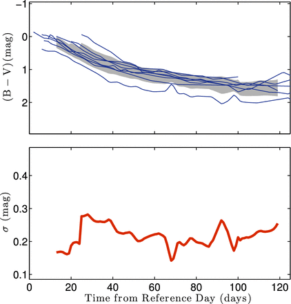
B − V colour, as a function of time (upper panel) and its standard deviation (bottom panel). Colour curves are aligned according to their explosion day. The shaded area represents ±1σ from the mean colour values. The scatter appears similar throughout the plateau.
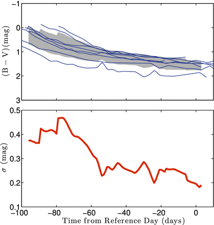
When the curves are aligned to the explosion day, the standard deviation remains generally constant over time, showing that there is no ‘preferred epoch’ with smaller scatter. When we set the zero time to the end of the plateau phase (e.g. as done by Olivares et al. 2010), σB − V at that origin is similar to what we had before, but rises dramatically as we move away towards earlier times. This indicates that not only intrinsic differences still exist at all plateau phases, but that the end of the plateau is not a natural origin for object comparison. This is consistent with a theoretical picture, where the precise end of the plateau will depend on envelope masses, velocities, nickel mass, and other specific properties of a given object (e.g. Kasen & Woosley 2009).
Nevertheless, we follow Hamuy (2005), take the end of the plateau as a reference point, and compare colours at that point to those of SN 1999em. We assume that any relative departure of the colour of a SN from SN 1999em is caused by dust. This SN has been extensively modelled by Baron et al. (2000) and others and has an upper limit of E(B − V)tot = 0.15 mag. This value also includes Milky Way reddening in the direction of SN 1999em (0.036 mag; Schlegel et al. 1998), so we adopt E(B − V)host = 0.12 mag. The results are shown in the last column of Table 4.
Extinction values extracted from the Na iD EW.
| SN name | EW|$_{\rm Na\,\small {I}D}$| (Å) | E(B − V)Tur016 | E(B − V)Bar025 | E(B − V)colour |
|---|---|---|---|---|
| 1999em | 1.43 | 0.22 ± 0.04 | 0.36 ± 0.06 | 0.12 |
| 1999gi | 0.92 | 0.14 ± 0.01 | 0.23 ± 0.02 | 0.33 |
| 2000bs | 0.97 | 0.15 ± 0.04 | 0.24 ± 0.07 | – |
| 2000dj | – | – | – | −0.09 |
| 2001cm | 0.73 | 0.11 ± 0.03 | 0.18 ± 0.04 | – |
| 2001X | 0.51 | 0.07 ± 0.01 | 0.13 ± 0.01 | 0.09 |
| 2002an | 0.43 | 0.06 ± 0.01 | 0.11 ± 0.01 | – |
| 2002gd | 0.92 | 0.14 ± 0.01 | 0.23 ± 0.02 | 0.27 |
| 2002hh | 2.75 | 0.43 ± 0.02 | 0.69 ± 0.03 | – |
| 2003hl | 2.00 | 0.31 ± 0.03 | 0.50 ± 0.05 | 0.57 |
| 2003iq | 1.33 | 0.20 ± 0.02 | 0.33 ± 0.03 | −0.03 |
| 2003Z | – | – | – | 0.19 |
| 2004du | – | – | – | 0.13 |
| 2004et | 1.67 | 0.26 ± 0.00 | 0.42 ± 0.01 | – |
| 2005ay | – | – | – | 0.11 |
Using the resulting E(B − V) values and the extinction curve of Cardelli, Clayton & Mathis (1989), we can estimate E(V − R) and E(R − I). In Fig. 5, we show the curves before and after the correction. The corrected B − V curves obviously meet at zero and show a gradual decline in scatter approaching the end of the plateau. This sample is small and does not allow for a definitive conclusion. However, one can see that while the scatter in the redder colours is marginally reduced, it is achieved by shifting two objects, at the cost of somewhat scattering the remainder of the sample. When SNe 1999gi and 2003hl are excluded from the analysis, the mean σ increases from 0.06 to 0.09 in V − R and from 0.04 to 0.06 in V − I. Since before any correction the scatter in colour is small, only highly accurate extinction values can have a chance to reduce it more.
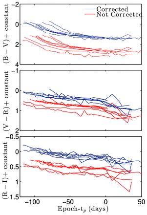
B − V, V − R, and R − I curves aligned to the end of the plateau phase, before, and after extinction correction by comparing to SN 1999em. Since B − V colour is used for correction, its scatter is obviously reduced (though not significantly at early times), but other bands hardly benefit from this correction.
3.2 The Na iD equivalent width
Early studies on SNe Ia have suggested that the equivalent width of the Na iD doublet, EW|$_{\rm Na\,\small {I}D}$|, is a good proxy for the amount of extinction towards a SN (Barbon et al. 1990; Turatto, Benetti & Cappellaro 2003). However, using a much larger sample, Poznanski et al. (2011) showed that although EW|$_{\rm Na\,\small {I}D}$| correlates with the extinction when measured from low-resolution spectra, there is so much scatter that the method is effectively useless. This is likely due to a combination of the doublet lines not being resolved, variations in observing conditions introducing different amounts of continuum light from the host galaxy, the effects of CS matter (Phillips et al. 2013), as well as intrinsic sources of scatter, such as variations in dust-to-gas ratios in different galaxy types (Issa, MacLaren & Wolfendale 1990; Lisenfeld & Ferrara 1998), the effects of depletion of metals on dust grains (e.g. Savage & Mathis 1979), and similar processes.
We collect from the literature four of the available dereddening relations: Barbon et al. (1990), |$E(B-V) = 0.25\,{\rm EW}_{\rm Na\,\small {I}D}$| (Bar025); the two linear relations derived by Turatto et al. (2003), |$E(B-V) = 0.16\,{\rm EW}_{\rm Na\,\small {I}D} - 0.01$| (Tur016) and |$E(B-V) = -0.04 + 0.51\,{\rm EW}_{\rm Na\,\small {I}D}$| (Tur051); and the relation derived by Poznanski et al. (2011): |$E(B-V) = -0.08 + 0.43\,{\rm EW}_{\rm Na\,\small {I}D}$| (Poz043). We note that we do not use the more recent relation from Poznanski, Prochaska & Bloom (2012), since it only holds for EW < 1 Å, and many objects in the sample exceed this value.
The EWs are measured using a similar method to the one described by Poznanski et al. (2011). We inspect the spectra visually, and when we detect a line, we identify its edges and pseudo-continuum manually. We fit a low-order polynomial to the continuum and divide the data by the continuum fit. We then perform a numerical integral on the normalized data to find the EW and measure the noise of the spectrum, N, defined as the 5σ clipped standard deviation around the flattened spectrum. We assume the uncertainty in EW to be dominated by N. We calculate the uncertainty, δEW, as δEW = N W/2, where W is the width of the line (defined as the distance in Å between the manually marked line limits). We divide by a factor of 2 to account for the approximately triangular shape of the feature. We average the EWs obtained from different spectra for every SN, except for SN 1999em for which we use only one spectrum, where the doublet lines were resolved, and we assume this particular spectrum to be more reliable than the rest of the spectra. We manage to detect Na iD in a total of 11 SNe, and their values appear in Table 4.
From the dereddened colour curves shown in Fig. 6, it is clear that Tur051 (with a slope that heavily depends on the single very reddened SN 1986G) and Poz043 only increase the scatter and therefore overestimate E(B − V). Tur016 reduces σ only by an insignificant 9 per cent and Bar025 by 7 per cent.
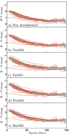
B − V colour curves of 12 SNe for which an Na iD absorption line is detected, dereddened according to various relations from the literature; a decrease in scatter is observed only in (b), where the average σ is reduced by 9 per cent, whereas (c) and (d) show an increase of 40 and 15 per cent (respectively) in scatter. The shaded area represents ±1σ from the mean colour.
Comparison of E(B − V) values extracted from the three methods that showed a modicum of success can be found in Table 4. The methods give different and typically inconsistent values, indicating that they are too often equivalent to an educated guess. Since all the methods seem to suffer from systematic uncertainties, any averaging between the results is nearly guaranteed to be wrong. With the exception of SN 2002hh (Pozzo et al. 2006), our SNe suffer rather moderate extinction, and we apply no dust correction in the following sections.
4 PHOTOMETRIC PROPERTIES
Pastorello et al. (2004) suggested that there are two distinct classes of SNe II-P, faint and bright (though see an update in Spiro et al. 2014). Fraser et al. (2011) further find that low-luminosity objects also tend to result from explosions of lower mass stars. In contrast, using all SNe II-P with measured progenitor masses, Poznanski (2013) finds that there is a correlation between the mass and ejecta velocity, and since velocity and luminosity are related as well, mass should correlate with luminosity. With the large uncertainties involved in mass determination, it is hard to determine whether what one sees is indeed a correlation in a one-parameter family or two distinct populations.
In Fig. 7, we show the I-band light curves for the entire sample. It is rather apparent that while it spans a range of 3 mag, there is a continuous distribution of luminosities, with at most a half-magnitude gap below M = −16 mag.
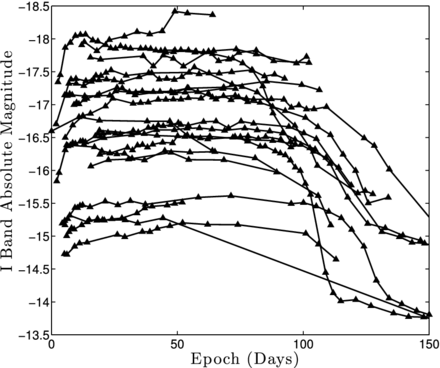
I-band light curves in absolute magnitude for the sample. The curves seem to continuously cover a range of the order of 3 mag (between −18 and −15 mag). However, plateau duration is rather uniform, near 100 d.
In the top panel of Fig. 8, we plot the I-band absolute magnitude on day 50 versus plateau length. We define the plateau duration as the time from explosion to the day where the light curve drops by 0.5 mag from the mean plateau value, which is longer than the actual time during which the photometric (or bolometric) luminosity is actually constant, but is more easily defined. We exclude objects with incomplete data (i.e. for which the light curves terminate before the post-plateau drop), so that we are ultimately left with nine objects. The analysis is done in the I band where the plateau is the most prominent. Plateau durations are rather similar for all objects, of the order of 100 d, reinforcing the findings of Arcavi et al. (2012) and Poznanski (2013). However, within the scatter, it is apparent that more luminous SNe have shorter plateaus, as predicted by Poznanski (2013). One should note that since we define the durations from explosion rather than peak brightness or some other metric, we tend to have plateaus that are a few days longer than other authors (e.g. Anderson et al. 2014b).
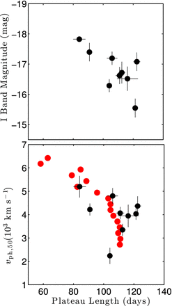
Top panel: I-band absolute magnitude on day 50 versus plateau duration. The plateau length stays approximately constant over a large range of magnitudes, though perhaps getting shorter for brighter SNe. Bottom panel: photospheric velocities on day 50 versus plateau duration. Since there is an established correlation between luminosity and velocity for SNe II-P, the plot resembles the one in the top panel. The red dots are a subset of grid models computed by Dessart et al. (2010), interpolated to satisfy the mass–velocity relation found by Poznanski (2013). These models show very good agreement with our measurements.
The luminosity of SNe II-P correlates with the day 50 photospheric velocity (Hamuy & Pinto 2002), and in the lower panel of Fig. 8 we plot the latter against the plateau length. We compare our results to a subset of grid models computed by Dessart, Livne & Waldman (2010), interpolated to satisfy the mass–velocity relation found by Poznanski (2013, red points). We can see a reasonable match between the models and our observations of SNe II-P, both consistent with a uniform plateau duration of ∼100 d up to a velocity ∼4500 km s−1, after which the plateaus tend to get shorter.
Various authors define the plateau duration differently and measure it in different bands. While it is beyond the scope of this work to quantitatively test this result with objects from the literature, we do note that when looking at a handful of such SNe we see a complex picture. While SNe 2003hn (Harutyunyan et al. 2008; Bersten & Hamuy 2009; Jones et al. 2009; Krisciunas et al. 2009) and 2012A (Tomasella et al. 2013) have markedly shorter plateaus and relatively high ejecta velocities, SN 2005ay (Tsvetkov et al. 2006; Gal-Yam et al. 2008) may not be consistent with that trend.
We also find that the decline rate of the I-band light curves correlates well with vph, 50, as seen in Fig. 9. A possible explanation is that high ejecta velocities will cause a fast decrease in density, which will be followed by a quicker release of radiation.
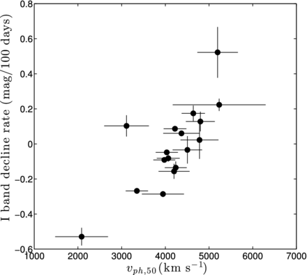
The I-band decline rate versus vph, 50. There is a clear correlation between the decline rate of the light curve and the photospheric velocity.
4.1 Colour evolution
Fig. 10 shows the colour evolution of the sample. At early times, the B − V colour declines sharply owing to the drop in temperature. This is because the bluer bands are in the Wien part of the blackbody spectrum and therefore more sensitive to temperature change. In addition, strong iron blanketing mostly affects bluer bands. However, during the recombination phase B − V changes moderately since the conditions at the photosphere remain approximately constant. For the same reason, V − R and R − I show almost no change. The larger scatter in B − V compared to redder colours could be due to extinction, but also to variations in metallicities that translate to a different amount of line blanketing.
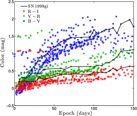
B − V, V − R, and V − I colour evolution of the whole sample. The individual curves of SN 1999gi are shown in black to guide the eye. The highly reddened object separated from the other curves is SN 2002hh.
At the end of the plateau phase, for the objects for which we have extending post-plateau data (SNe 1999em, 2001X, and 2003gd) one can see a turnover in B − V as shown in Fig. 11. In SNe 2001X and 2003gd, we also see a marginal B-band brightening, of the order of 0.1–0.2 mag at one and three epochs, respectively. We tentatively suggest that this might be related to the prediction of Chieffi et al. (2003), who calculate that this may occur due to the rising helium abundance in the photosphere, which decreases the recombination temperature and causes a rapid release of energy.
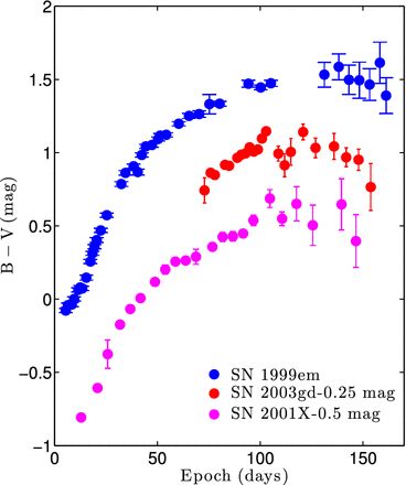
SNe for which we have post-plateau measurements exhibit a phase of rising B − V colour after the end of the plateau. This behaviour was predicted by Chieffi et al. (2003), and it might be the result of the rising helium abundance in the photosphere, which decreases the recombination temperature and causes a more rapid release of energy.
4.2 Rise time
It is usually hard to detect a SN II-P during its early rise to maximum brightness owing to the rapid nature of this stage, so light curves usually begin on the plateau. Luckily, four of our SNe II-P were detected sufficiently early to reveal part of the rise, and we display their R-band light curves in Fig. 12. Our data show that most of the rise time to maximum brightness occurs within a handful of days, after which the emission settles on to the plateau within a few more days; however, there are significant variations in the light-curve shapes.
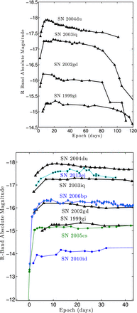
Upper panel: R-band light curves of the four events for which we have captured the early rise to the plateau. SN 2004du is the only one that also has an early bump peaking ∼12 d past explosion. Lower panel: the early R-band light curves of eight SNe. The rise time and the absolute magnitude on the plateau do not show an obvious correlation.
Gal-Yam et al. (2011) suggest a correlation between the rise time of SNe II-P and their luminosity. They show that two underluminous events (SN 2005cs and SN 2010id) rise sharply to the plateau, compared to the more luminous SN 2006bp. To the four SNe in our sample for which we have early-time data, we add the recent SN 2013ej from Valenti et al. (2014) and the events used by Gal-Yam et al. (2011): SN 2006bp (Quimby et al. 2007) and SN 2010id (Gal-Yam et al. 2011). We also add from Pastorello et al. (2009) early data for SN 2005cs, in order to cover the earliest parts of the light curve. The early-time data for SN 2005cs were collected by amateur astronomers and were taken from the Astrosurf website.5 These data were rescaled by Pastorello et al. (2009) to V- and R-band magnitudes.
Fig. 12 shows the R-band evolution of this largest sample ever compiled of early-time SN II-P light curves. Upon visual inspection, no striking correlation between rise time and luminosity emerges. A quantitative assessment will be inconclusive, owing to the still small sample size, the sparse sampling of the light curves, and difficulty defining the endpoint consistently due to the large variance in light-curve shapes.
The plateau starts once the temperatures drop below ∼8000 K. It implies, based on equation 31 of Nakar & Sari (2010), that the time to the plateau (roughly the rise time) is trise ∝ M−0.23 E0.2 R0.68. Taking E ∝ M3, M ∝ v, and L ∝ v2 (Poznanski 2013) implies trise ∝ L0.18R0.68. As we see, the dependence of the rise time on luminosity is weak, and most of the variance would come from differences in radii. However, due to the large luminosity range, and assuming that the radii do not correlate with luminosity (which is probably wrong), one can still get a factor of 2 variation in the rise time, which we cannot rule out.
5 SPECTROSCOPIC COMPARISON
In Figs 13 and 14, we show the spectral evolution of our sample of SNe II-P until the end of the plateau phase. In each panel, we plot a representative subsample of our spectra in the indicated range of epochs including line identifications. The spectral lines were identified using the local thermodynamic equilibrium (LTE) synthetic spectra of Hatano et al. (1999). We compared the synthetic spectrum of various ions to our spectra, looking for coinciding lines. Candidate ions were those whose optical depth is close to unity at the temperature of the photosphere, which we assumed to be in the range of 6000–10 000 K. Once a feature was associated with a specific species, we searched for other strong lines of the same ion in the spectrum in order to confirm or reject the identification. When several species blend, we order them by the importance of their contribution.
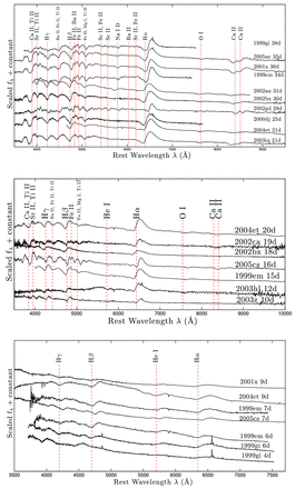
Representative spectra 0–40 d after explosion. Dashed vertical lines indicate the wavelengths of the specified species displaced by the mean Fe ii velocities during those epochs and by the mean Hα velocities for Balmer lines. Early spectra before day 10 are very hot and display only Balmer (Hα, Hβ, and Hγ) and He i λ5876 P-Cygni profiles. Between days 10 and 20, the spectra flatten and lines of heavier species appear. All absorption and emission lines are very broad due to high velocity dispersion. Absorption lines are enhanced as well as emission lines towards mid-plateau phases.
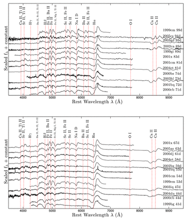
Same as Fig. 13, for 40–100 d past explosion. Absorption and emission lines are clearly stronger towards mid-plateau phases. As a SN approaches the nebular phase and temperatures drop, one can see reduced absorption and an enhancement of line emission.
The first panel of Fig. 13 displays the early hot days of the SNe, where the spectra are very blue and only few lines are present. Balmer (Hα, Hβ, and Hγ) and the Na iD (blended with He I) lines exhibit prominent and broad P-Cygni profiles, with blueshifted emission components in the Hα and Hβ profiles.
In Fig. 15, we illustrate the evolution of Hα and Hβ for three SNe, selected for having multiple spectra (SN 2004et, SN 2001cm, and SN 2001X). The absorption and emission features are very broad owing to large dispersion in the ejecta velocities. The absorption full width at half-maximum intensity is ∼5000–6000 km s−1 around day 25. The deviation of the emission peak from the rest wavelength is substantial during the first days and reaches ∼2000–3000 km s−1 around day 20, after which it declines. On day 57 the shift is only ∼540 km s−1 for SN 2004et and it completely disappears by day 117. SN 2001cm behaves similarly, whereas SN 2001X is still blueshifted by ∼250 km s−1 on day 181. The assumption of a spherically symmetric expansion should lead to the formation of a symmetric emission profile around zero velocity, in contrast to what we actually see. Dessart & Hillier (2005a) explain these observations using the cmfgen model atmosphere code (Hillier & Miller 1998), which solves the radiative transfer and statistical equilibrium equations in an expanding medium, assuming radiative equilibrium. They show that the blueshift of the emission peak arises from the combined effect of disc occultation and a line-forming region very close to the photosphere. The confinement of that region to the photosphere causes a significant flux deficit in the red side of the emission profile, which is enhanced for rapidly declining density profiles, like the ones assumed for CC-SNe. The offset of the emission peak from zero velocity declines with time, as the occulted region becomes smaller with the photosphere's recession into the star. These blueshifts are discussed in detail by Anderson et al. (2014a).
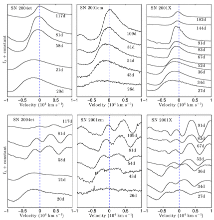
P-Cygni profiles of Hα (upper panel) and Hβ (lower panel) for three SNe: SN 2004et, SN 2001cm, and SN 2001X. The emission component is blueshifted by ∼2000 km s−1 in early spectra (around day 20), but as the SN evolves with time the shift decreases, and it almost disappears when the SNe approach the nebular phase.
By day 10 the temperature drops and the continuum flattens, and around day 15, Fe ii λ5169 and the Ca ii lines emerge along with O i λ7774. By day 20 we can already see a strong line of Ba ii λ4554 (probably blended with Fe ii and Ti ii) and a hint of what appears to be Sr ii λ4077 (blended with Ti ii).
During this range of epochs, most spectra are not yet very developed. However, SN 2005cs shows many details quite early relative to other objects (e.g. see the spectrum at day 16 in Fig. 13). Around day 10, a notch appears in the Hα blue wing of several SNe. This feature, possibly due to hydrogen at high velocity (HV), gets stronger and remains visible until the end of the plateau phase. We will discuss this matter in detail in Section 6.
A few more lines appear near day 35, where we can perhaps see Ba ii λ6141 and Sc ii λλ6305, 5672, 5520, which are strongest for SN 2005cs. On the second half of the plateau and towards its end, the strong Balmer Hβ and Hγ lines, as well as Ca ii H&K, become wider and less distinct owing to blending with (perhaps) Ti ii and Fe ii, and are thus much more difficult to detect. One can also notice the growing emission lines along with the reduction of the absorption components, as the SNe approach the nebular phase.
The absorption EW of the hydrogen lines grows approaching mid-plateau epochs and declines towards the nebular phase. The general shape of the evolution can be interpreted as follows. When the SN is young and hot, the hydrogen is fully ionized and its optical depth at the photosphere is close to 1, generating only little absorption. When the photosphere cools and hydrogen atoms start recombining with electrons, the optical depth approaches ∼1000, and simultaneously more material is revealed as the photosphere recedes, bringing the line profile to maximal absorption. By the end of the plateau phase, the density is small enough to increase the probability of photon escape without going through absorption in hydrogen atoms, and the EW decreases slowly. We discuss this further in Faran et al. (2014).
5.1 Ejecta velocities
We measure the velocities of Hα, Hβ, and Fe λ5169 in every spectrum where they can be detected. We do so by fitting a third-order polynomial to the absorption component of the P-Cygni line, and taking its minimum as the centre of the velocity distribution. We do not rectify the lines owing to the difficulty in defining the continuum around the profiles, which might cause systematic errors in our measurements. In order to estimate measurement uncertainties, we smooth the data using a Savitzky–Golay filter (Savitzky & Golay 1964). We then divide our spectra by their smoothed versions, thus generating a vector of noise. We randomly mix the noise vector in wavelength to create 104 different vectors. Each artificial noise spectrum is then multiplied by the smoothed spectrum to create a ‘new’ spectrum of signal plus noise, and the velocity is measured for every one of these. The standard deviation of the results gives us the uncertainty in the original velocity measurement and is typically ∼70 km s−1 when the signal to noise is high. This is probably an underestimate, but an uncertainty of 250 km s−1 is added in quadrature to account for peculiar velocities. We linearly interpolate (or extrapolate) the velocities of each object to day 50 after explosion and normalize the measurements by that value.
Hα and Hβ are detected at high velocities in early epochs and are emitted from the outer ejecta. Lower velocity layers are revealed as the photosphere recedes and lines of heavier ions emerge. The velocity of the photosphere can be traced using the Fe ii triplet, which is believed to be generated at the thermalization surface, and is therefore considered a good proxy for the velocity near the photosphere (Schmutz et al. 1990; Dessart & Hillier 2005b).
The temporal evolution of the various scaled velocities is well fitted by power laws as can be seen in Fig. 16, where we use only spectra obtained before day 150. Uncertainties in the explosion date are also taken into account in the calculation. The Fe ii velocity declines with a power of β = −0.581 ± 0.034, a somewhat sharper decline than the −0.464 ± 0.017 found by Nugent et al. (2006). Since they used a narrower time window, we repeat our fit using only spectra obtained between days 9 and 75, but we obtain roughly the same sharp decline as we did using all of our data. The difference might be caused by our better sampling of the early days, where the decline is significant and can change the fit most effectively. Overall, we can represent the SN II-P evolution of the velocities as |$v_{\rm Fe\,\small {II}}=v_{\rm ph,50}\,(t/50)^{-0.581\pm 0.034}$|, vHα = vph, 50 (t/50)−0.412 ± 0.020, and vHβ = vph, 50 (t/50)−0.529 ± 0.027.
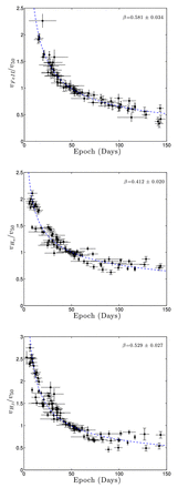
Fe ii λ5169 (top panel), Hα (middle), and Hβ (bottom) velocities normalized by vph, 50. Best-fitting power laws are plotted with dashed lines. All SN II-P velocities follow their respective power laws quite well and with little scatter.
Our results show that |$v_{\rm Fe\,\small {II}}$| and vHβ follow a similar power law, and are thus linearly related, as was already shown by Poznanski et al. (2010) and earlier explored by Nugent et al. (2006). This allows vHβ to be a proxy for the photospheric velocity at early epochs, when the Fe ii lines have not yet emerged. We fit a power law of the form |$v_{\rm Fe\,\small {II}} = a\,v_{\rm H}^{-b}$| using 79 spectra of 20 SNe for which all the velocities are measurable. We restrict the velocities to epochs earlier than 200 d. We find that |$v_{\rm Fe\,\small {II}}$| is indeed linearly proportional to Hβ with a power law of b = 1.01 ± 0.01. Fitting a linear function, we find that |$v_{\rm Fe\,\small {II}} = (0.805 \pm 0.006)v_{\rm H\beta }$| with χ2/dof = 1.72. This agrees with the results of Poznanski et al. (2010). On the other hand, vHα follows Fe ii with a power law of b = 1.32 ± 0.02. Nevertheless, fitting a linear function, we find that |$v_{\rm Fe\,\small {II}} = (0.855 \pm 0.006)v_{\rm H\alpha } - (1499 \pm 87)$| km s−1 with χ2/dof = 2.23. Both fits to the data are shown in Fig. 17.
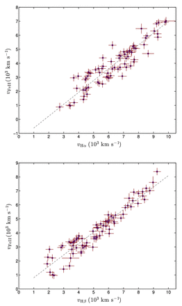
Fe ii λ5169 velocities versus Hα (upper panel) and Hβ (lower panel) velocities. |$v_{\rm Fe\,\small {II}}$| is linear with vHβ, and the best-fitting gives |$v_{\rm Fe\,\small {II}} = (0.805 \pm 0.005)v_{\rm H\beta }$|. While the vHα evolution is different from |$v_{\rm Fe\,\small {II}}$|, their dependence can still be approximated by a linear relation, |$v_{\rm Fe\,\small {II}} = (0.855 \pm 0.006)v_{\rm H\alpha } - (1499 \pm 87)$| km s−1.
6 HV FEATURES
Eight different objects at various epochs during their photospheric phase (day 14 or earlier in SN 1999em, day 81 in SN 2001cm) have a blue notch in Hα, which could be HV hydrogen features. Alternatively, it could be Si ii λ6355. If these are indeed HV features, one should expect to find similar absorption in the profiles of other hydrogen lines. In Fig. 18, we compare the spectra that show the feature near Hα (black) as well as near Hβ (red). The presence of an additional absorption supports the identity of the lines as HV features, as discussed by Inserra et al. (2012) who identified similar features in the spectra of SN 2009bw. Note that for SN 2001X, the velocities of the Hα and Hβ components do not match, and the identification as HV features is therefore dubious. The HV lines follow the redward drift with time like the rest of the spectral lines.
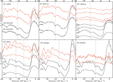
Spectra of six SNe showing the HV features in Hα (black) which have a counterpart in Hβ (red). The HV components are seen at high velocities of ∼−10 000 km s−1 and slow down with time. The presence of matching line in Hβ supports an interpretation of a hydrogen HV feature.
In Fig. 19, we show the spectra of two SNe where no counterpart is detected in Hβ. The spectrum of SN 2002ca has low signal-to-noise ratio, which might affect our ability to detect the Hβ component, but that is not the case for the other SN. We therefore favour an interpretation of Si ii λ6355 at a velocity of ∼5000 km s−1, typical to metals in SNe II. In a similar case, Valenti et al. (2014) see a wide absorption feature in SN 2013ej on the blue side of Hα without a counterpart in Hβ, and interpret it as a line of Si ii λ6355. However, it is much stronger than the lines in our sample.
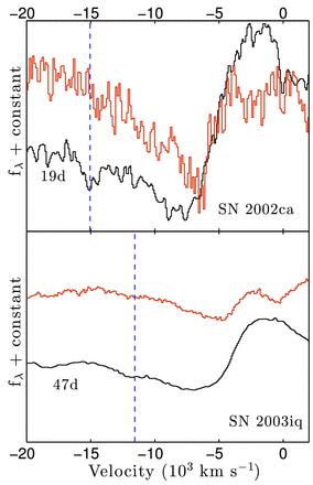
Same as Fig. 18 for SNe with a blue notch in Hα but not in Hβ, favouring the interpretation as Si ii λ6355.
It is interesting to follow the time evolution of the Hα HV feature in the spectra of SN 1999em. As seen in Fig. 20, the feature is first evident in the ninth spectrum on day 15, and appears relatively strong and wide at a velocity of ∼−15 000 km s−1. It is still present on the subsequent day, but completely disappears 10 d later. A new HV feature appears again between days 34 and 38, but this time it is much narrower and does not resemble the previous feature in shape. The notch remains apparent at least until the SN enters the nebular phase. We do not see this behaviour in the HV feature we associated with Hβ, as it emerges only at days 34–38, together with the Hα HV notch. The complete disappearance and the different shape of the line after it reappears suggest that the feature comes from two different emission regions or mechanisms dominating at different epochs. However, since no counterpart in Hβ is found before days 34–38, the early feature might be associated with Si ii λ6355 and not HV hydrogen.
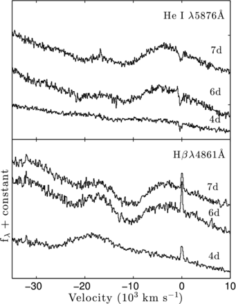
Early-time HV features associated with Hβ and He i λ5876 in SN 1999gi. The HV components are observed at high velocities of ∼−20 000 km s−1, with a P-Cygni profile.
HV features are also present during early phases near the Hβ and He i λ5876 profiles of SN 1999gi (Leonard et al. 2002b), and in the Hβ absorption of SN 1999em (Baron et al. 2000; Leonard et al. 2002a) and SN 2001X. Figs 21 and 22 show the early-time spectra of SNe 1999gi, 1999em, and 2001X around those lines. The line near 5800 Å is most likely a product of He i and not Na iD, especially if non-LTE effects are responsible for these lines (Baron et al. 2000). If these features are indeed associated with hydrogen and He i λ5876, they appear at much higher velocities than those measured in later epochs. In Figs 21 and 22, both the Hβ and the He i λ5876 profiles of SN 1999gi on days 6–7 and day 9 in SN 2001X reveal what seems to be a second P-Cygni profile, containing both an emission peak and an absorption dip, at ∼−25 000 km s−1. Alternatively, Dessart et al. (2008) identify the HV feature in SN 1999gi as He ii λ4686.
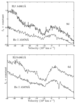
Early-time HV features of SN 2001X (top) and SN 1999em (bottom) near Hβ and He i λ5876. The Hβ line presents a quite prominent HV absorption line, which is missing from the He i line.
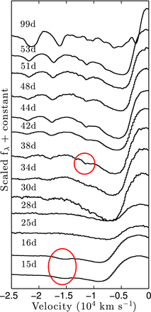
The evolution of the HV feature in the Hα blue wing of SN 1999em. An HV component is evident in the first two lower spectra at a velocity of ∼−15 000 km s−1, and it disappears on day 25. It suddenly reappears in the spectrum of day 38 and remains visible until the end of the plateau phase.
There have been several attempts to explain the origin of these strange features. Using synow, Baron et al. (2000) identified them as HV absorption of hydrogen in the spectra of SN 1999em. They further raised the hypothesis that these are ‘complicated P-Cygni profiles’, created by non-LTE effects which alter the Balmer level populations in the mid-velocity range, and create two line-forming regions of hydrogen and helium. Alternatively, these lines could be more easily explained by N ii if there is a steep density gradient, as later advocated by Dessart & Hillier (2005a).
Chugai, Chevalier & Utrobin (2007), on the other hand, suggest that interaction of the ejecta with a typical red supergiant wind leads to the formation of those features. They develop a model for the ionization and excitation of H and He in the unshocked ejecta, considering time-dependent effects and the irradiation of ejecta by X-rays in order to study the signs of CS interaction.
They base their diagnosis of CS interaction on spectroscopic observations of Hα and He i λ10 830 at the photospheric phase of SN 1999em and SN 2004dj. In their model, the interaction between the SN ejecta and the circumstellar material (CSM) results in the formation of forward and reverse shocks, which emit X-rays and ionize and excite the outer recombined layers of the unshocked ejecta. This interaction is too weak to be revealed through specific emission lines in SNe II-P, but sufficient to be detected as HV absorption features in the blue wing of Hα and He i λ10 830. This process causes the emergence of HV absorption in the blue wing of Hα at t ≈ 40–80 d and another component in He i λ10 830 at ∼20–40 d, both at a radial velocity of ∼104 km s−1. The depth of these features increases with wind density. Chugai et al. (2007) measured a much lower velocity for SN 2004dj than SN 1999em (8200 versus 11 500 km s−1). Based on this, they ruled out the possibility that the line was an unidentified metal line. Similar differences in velocities at comparable epochs can be seen in Fig. 18.
Chugai et al. (2007) further suggest an additional mechanism to account for the narrow notch that appears in mid-plateau spectra of SN 1999em and SN 2004dj. They raise the possibility that a cool, dense shell might form at the interface between the SN and the CSM through radiative cooling. When the shell is excited by X-rays, it can produce narrow HV absorption components in Hα. This produces two components: a narrow notch, created in the weakly perturbed shell, and a broad notch originating in the area of Rayleigh–Taylor instability occurring in a decelerating shell (the instability increases the turbulent velocity and broadens the line). Those components are distinguished from the effect of the ionized unshocked ejecta discussed previously, which produces a broader shallow absorption. We detect the narrow notch in the Hα profile of SN 1999em around day 50 and also in spectra of SN 2001cm (day 81 – earliest spectrum), SN 2001X (day 91, in both features), and SN 2003hl (day 73). This interpretation explains the evolution of the HV feature in SN 1999em described above.
7 CONCLUSIONS
Our photometric and spectroscopic analysis of a sample of 23 SNe II-P reveals the following.
The luminosity distribution of SNe II-P seems continuous, spanning 3 mag, as numerous authors have shown in the past and more recently (e.g. Hamuy 2003; Anderson et al. 2014b; Sanders et al. 2014; Spiro et al. 2014).
Plateau durations are typically 100 d, but we find preliminary indications that they get shorter for more luminous, energetic SNe, as expected from Poznanski (2013).
Using a sample of eight SNe, the largest to date, we do not find obvious support to the claim of a correlation between rise time and plateau luminosity as previously suggested by Gal-Yam et al. (2011) and Valenti et al. (2014); however, we cannot rule it out, mostly due to the large variance in light-curve shapes.
Three SNe tentatively show a post-plateau colour change and rebrightening, which could perhaps be interpreted as being caused by helium recombination (Chieffi et al. 2003).
We find that hydrogen and iron velocities follow well-behaved power laws, with little scatter, as shown by Nugent et al. (2006), though we derive a somewhat steeper decline using a much larger sample.
Signs of interaction with CSM might be evident in the spectra of at least six events, where we find HV features in the blue wing of Hα during the plateau phase. Corresponding absorption in Hβ reinforce the interpretation that these are indeed HV lines associated with hydrogen and not metal lines. However, other interpretations are possible.
When studying SNe, there are a multitude of methods used in the literature to correct for dust extinction: photometric methods based on comparison to low-extinction SNe or spectroscopic ones using the Na iD doublet. With the availability of a sample, we were given the opportunity to ask a simple question: Does the uniformity of the sample increase after the application of a given method? Any reasonably behaved underlying distribution should become tighter after correction. The uniform answer was negative; no method we tested made a significant improvement. This is likely due to a combination of the weakness of the methods (i.e. the intrinsic scatter they introduce) and modest typical extinction of SNe II, of the order of ∼0.2 mag.
We thank D. Maoz I. Arcavi, and the referee for helpful comments on this manuscript. A. Barth, A. Coil, E. Gates, B. Swift, and D. Wong participated in the many observations that made this work possible, and we thank them for it. Some of the data presented herein were obtained at the W. M. Keck Observatory, which is operated as a scientific partnership among the California Institute of Technology, the University of California, and the National Aeronautics and Space Administration; it was made possible by the generous financial support of the W. M. Keck Foundation. We wish to recognize and acknowledge the very significant cultural role and reverence that the summit of Mauna Kea has always had within the indigenous Hawaiian community. We are most fortunate to have the opportunity to conduct observations from this mountain. The Kast spectrograph on the Shane 3 m reflector at Lick Observatory resulted from a generous donation made by Bill and Marina Kast. We also thank the dedicated staffs of the Lick and Keck Observatories for their assistance. This research made use of the Weizmann interactive supernova data repository (www.weizmann.ac.il/astrophysics/wiserep), as well as the NASA/IPAC Extragalactic Database (NED) which is operated by the Jet Propulsion Laboratory, California Institute of Technology, under contract with NASA.
KAIT (at Lick Observatory) and its ongoing operation were made possible by donations from Sun Microsystems, Inc., the Hewlett-Packard Company, AutoScope Corporation, Lick Observatory, the NSF, the University of California, the Sylvia & Jim Katzman Foundation, and the TABASGO Foundation. DP acknowledges support from the Alon fellowship for outstanding young researchers, and the Raymond and Beverly Sackler Chair for young scientists. DCL acknowledges support from NSF grants AST-1009571 and AST-1210311. JMS is supported by an NSF Astronomy and Astrophysics Postdoctoral Fellowship under award AST-1302771. AVF's group at UC Berkeley has received generous financial assistance from the Christopher R. Redlich Fund, the Richard and Rhoda Goldman Fund, the TABASGO Foundation, and the NSF (most recently through grants AST-0908886 and AST-1211916).
This paper is dedicated to the memory of our dear friend and colleague, Dr Weidong Li, without whom these data would not exist.
The NASA/IPAC Extragalactic Database (NED) is operated by the Jet Propulsion Laboratory, California Institute of Technology, under contract with the National Aeronautics and Space Administration (NASA).
REFERENCES
SUPPORTING INFORMATION
Additional Supporting Information may be found in the online version of this article:
Table 2. Sample journal of spectroscopic observations.
Table 3. Partial photometric data of the KAIT sample (Supplementary Data).
Please note: Oxford University Press is not responsible for the content or functionality of any supporting materials supplied by the authors. Any queries (other than missing material) should be directed to the corresponding author for the article.
Author notes
Deceased 2011 December 12.
NSF Astronomy and Astrophysics Postdoctoral Fellow.
