


Abstract
We investigate the structure of self-gravitating discs, their fragmentation and the evolution of the fragments (the clumps) using both an analytic approach and three-dimensional radiation hydrodynamics simulations starting from molecular cores. The simulations show that non-local radiative transfer determines the disc temperature. We find the disc structure is well described by an analytical model of a quasi-steady self-gravitating disc with radial radiative transfer. Because the radiative process is not local and radiation from the interstellar medium cannot be ignored, the local radiative cooling is not balanced with the viscous heating in a massive disc around a low-mass star. In our simulations, there are cases in which the disc does not fragment even though it satisfies the fragmentation criterion based on disc cooling time (Q ∼ 1 and Ωtcool ∼ 1). This indicates that, at least, the criterion is not a sufficient condition for fragmentation. We determine the parameter range for the host cloud core in which disc fragmentation occurs. In addition, we show that the temperature evolution of the centre of the clump is close to that of typical first cores, and that the minimum initial mass of clumps is about a few Jupiter masses.
1 INTRODUCTION
Stars form in gravitationally collapsing molecular cloud cores. Since molecular cloud cores have angular momentum (Goodman et al. 1993; Caselli et al. 2002), a circum-stellar disc forms around the protostar. According to recent theoretical studies of the gravitational collapse of molecular cloud cores, the protostar is surrounded by a circum-stellar disc early in its evolutionary phase when there is no magnetic field (Bate 1998; Machida, Inutsuka & Matsumoto 2010; Tsukamoto & Machida 2011) and when there is a magnetic field (Inutsuka, Machida & Matsumoto 2010; Machida, Inutsuka & Matsumoto 2011).
As Inutsuka et al. (2010) pointed out, a circum-stellar disc can be gravitationally unstable during its early evolution. When the protostar forms, its mass is only 10−2 to 10−3 M⊙. In contrast, the first core that is the precursor to the circum-stellar disc (Saigo & Tomisaka 2006; Machida et al. 2010) has an initial mass of ∼0.1 M⊙. Therefore, in the formation epoch of the protostar, the disc has a mass that is significantly greater than that of the protostar. Observations also suggest that massive discs can form in the main accretion phase (Enoch et al. 2009).
Disc fragmentation is a candidate mechanism for the formation of wide-orbit planets (Vorobyov & Basu 2010a; Machida et al. 2011; Vorobyov, DeSouza & Basu 2013). Wide-orbit planets are planets separated from the central star by more than 10 au (Marois et al. 2008; Lagrange et al. 2009; Thalmann et al. 2009; Lafrenière, Jayawardhana & van Kerkwijk 2010; Marois et al. 2010). Furthermore, it has been suggested that disc fragmentation can explain the formation of brown dwarfs (Stamatellos & Whitworth 2009a; Stamatellos et al. 2011a) and multiple stellar systems (Machida et al. 2008; Kratter et al. 2010).
The effects of radiative cooling on GI and disc fragmentation have been investigated by Gammie (2001) with two-dimensional local shearing box simulations. To model radiative cooling, he employed a simplified cooling law (see the last expression in (6)). In his simulations, the disc is initially unstable against GI (Q = 1) and GI immediately develops and heats the disc. When radiative cooling is not so strong, it balances the heating by GI, and the disc settles into a quasi-steady state. This quasi-steady state is also realized in three-dimensional global disc simulations (Lodato & Rice 2004). On the other hand, when radiative cooling is sufficiently strong, such a quasi-steady state cannot be realized and the disc fragments. In the simulations of Gammie (2001), disc fragmentation occurred when the disc cooling time tcool is comparable to the orbital timescale, tcool ∼ torbit (or Ωtcool ∼ O(1)). This fragmentation condition is also confirmed by three-dimensional global disc simulations (Rice et al. 2003) and the simplified cooling law was used.
Since Gammie (2001) and Lodato & Rice (2004) employed the simplified cooling law, they implicitly assumed that radiation just acts as a cooling process to decrease the local gas energy (we call this the assumption of local radiative cooling). However, this assumption is not necessarily true. For example, irradiation from the protostar and from the inner disc region can heat the disc. Thus, in reality, the incoming radiation flux, in addition to the outgoing radiation flux and local GI heating, should be considered. Furthermore, the interstellar medium has a typical temperature of about 10 K and it is almost impossible to cool the disc gas below 10 K because of the radiation flux from the ambient interstellar medium. Therefore, it is not clear that, in realistic situations, the local balance between radiative cooling and viscous heating is achieved or not as in Gammie (2001). Whether the balance is achieved is very important because the structure of a quasi-steady self-gravitating disc can be determined by the energy balance.
Another important issue is the applicability of the fragmentation criterion found by Gammie (2001), Q ∼ 1 and Ωtcool ∼ 1, for realistic situations. Gammie pointed out that, in realistic systems, fragmentation is realized when the external irradiation quickly diminishes and when the gas quickly cools. Thus, he regarded the fragmentation criterion as being applicable in very limiting cases.
On the other hand, Rice et al. (2003) interpreted this criterion as that ‘almost isothermal conditions are necessary for fragmentation’. When the cooling timescale of the disc is small, the gas evolves isothermally during the growth of GI and the pressure repulsion becomes weak compared to the adiabatic evolution case (or the inefficient cooling case). Rice et al. (2003) suggested that such almost isothermal evolution in the non-linear evolution phase of GI is necessary for fragmentation. According to this interpretation, how Q ∼ 1 is realized for the disc and the energy balance within it are not important because whether fragmentation is realized or not depends on the thermal behaviour of the gas in the non-linear evolution of the GI. The criterion seems to be a necessary condition in this interpretation.
In the previous works using an analytic approach, however, the criterion was used as if it were a sufficient condition for fragmentation (Rafikov 2005; Forgan & Rice 2011, 2013; Kratter & Murray-Clay 2011). As just described above, the interpretation of the criterion is ambiguous and its applicability for a realistic situation is still not clear.
Another mechanism that makes a disc gravitationally unstable is mass loading from the envelope (e.g. Matsumoto & Hanawa 2003; Inutsuka et al. 2010; Kratter et al. 2010; Vorobyov & Basu 2010a; Machida et al. 2011; Tsukamoto & Machida 2011; Bate 2011; Stamatellos, Whitworth & Hubber 2011b; Tsukamoto, Machida & Inutsuka 2013b; Tsukamoto & Machida 2013). This mechanism is efficient in the early phase of disc evolution during which the protostar and disc are embedded in a massive envelope. With mass accretion from the envelope, the Q value of the disc decreases due to the increase of the surface density. When the mass accretion on to the disc is sufficiently high, the disc eventually fragments, and planetary mass clumps form. In this process, whether fragmentation occurs depends on envelope (or cloud core) parameters such as thermal energy or rotational energy. The parameter range in which fragmentation occurs was investigated in our previous studies (Tsukamoto & Machida 2011, 2013); however, in those studies, the effects of radiative transfer were approximated. Radiative transfer could also play important roles during the early phase of disc evolution; therefore, a parameter survey of disc fragmentation with a radiation hydrodynamics simulation is necessary.
Initial properties and the evolution of fragments (or clumps) are other important issues. The ultimate fate of clumps depends on their orbital and internal evolution. For example, if the radial migration timescale is very short, clumps quickly accrete on to the protostar and disappear. If the radial migration timescale is sufficiently long and the clumps survive in the disc maintaining its mass in the range of planetary masses (≲ 10MJupiter), the clumps evolve into wide-orbit planets (Vorobyov & Basu 2010a; Machida et al. 2011). If the mass of the clumps quickly increases, disc fragmentation can be regarded as the formation process for brown dwarfs and binary or multiple stellar systems (Stamatellos & Whitworth 2009a).
In spite of its importance, only a few studies have focused on the orbital and internal evolution of clumps in circum-stellar discs. Baruteau, Meru & Paardekooper (2011) investigated the orbital evolution of massive planets in a gravitationally unstable disc under the assumption of local radiative cooling. They showed that massive planets rapidly migrate inward in a type I migration timescale (Tanaka, Takeuchi & Ward 2002). By adopting an analytical approach or three-dimensional smoothed particle hydrodynamics (SPH) simulation, Nayakshin (2010) and Galvagni et al. (2012) investigated the internal evolution and the collapse timescale of an isolated clump. The gravitational collapse (the second collapse) occurs in the clump when the central temperature reaches ∼2000 K, at which the dissociation of molecular hydrogen begins, and the gas pressure can no longer support the clump against its self-gravity. These authors suggested that the timescale for the second collapse after clump formation is in the range of several thousand years to several 104 yr. However, they ignored further mass accretion from the disc on to the clumps.
Tsukamoto et al. (2013b) investigated the orbital and internal evolution of clumps, permitting realistic gas accretion from the disc on to clumps with a three-dimensional radiation hydrodynamics simulation. They showed that although most of the clumps rapidly migrate inward and finally fall on to the protostar, a few clumps can remain in the disc. They also showed that clumps are convectionally stable (γ > γeff). The central density and temperature of a surviving clump rapidly increase, and the clump undergoes a second collapse within 1000–2000 yr after its formation. However, in this work, only one simulation was performed. The evolution of clumps may change under different initial conditions. For example, the central entropy of the clump could become small when fragmentation occurs in the outer relatively cold region of the disc. Since the central entropy of the clump determines its initial mass and the radius of the clump, different disc environments change the nature of the clumps. It is also expected that the mass accretion from the disc on to clumps becomes small when fragmentation occurs in the outer region where the disc surface density is small for Q = 1.
In this study, we investigate the structure of self-gravitating discs, fragmentation of the disc and the evolution of clumps using both an analytic approach and radiation hydrodynamics simulations starting from molecular cloud cores. This paper is organized as follows. In Section 2, we analytically derive the structure of a self-gravitating steady disc using various energy balance relations. It would be insightful to understand the general structure of self-gravitating discs. The numerical method and initial conditions for the simulations are described in Section 3. Results and discussions are divided into two parts (Sections 4 and 5). In Section 4, we mainly investigate the structure of a self-gravitating disc that formed in the radiation hydrodynamics simulations. The simulation results for disc evolution are presented in Section 4.1. In this section, we show that radiation can transfer energy within the disc and can heat the outer region of the disc. Therefore, the assumption of local radiative cooling is not valid in the disc. In Section 4.2, we discuss the consequences of the results obtained from our numerical simulations and their implications in interpreting previous work. In Section 5, we investigate disc fragmentation and the evolution of clumps. In Section 5.1, simulation results are shown. The parameter range of the molecular cloud core in which fragmentation occurs is determined, and the orbital and internal evolution of clumps is investigated. In Section 5.2, we discuss the results reported in Section 5.1 and derive the minimum initial mass of clumps. Finally, we summarize our results and discuss future perspectives in Section 6.
2 STRUCTURES OF SELF-GRAVITATING STEADY DISCS WITH VARIOUS ENERGY BALANCE EQUATIONS
An analytical description of the radial structure of a self-gravitating steady disc is useful for interpreting the simulation results shown in this study and in previous studies. In this section, we derive radial profiles for physical quantities in a self-gravitating circum-stellar disc using various energy balance equations. We assume that the disc: (1) is steady (|$\dot{M}={\rm const.}$|), (2) can be described by the viscous α accretion disc model (Shakura & Sunyaev 1973) and (3) is in the quasi steady-state against GI (Q ∼ 1).
Equations (5) shows that only a globally isothermal disc can achieve a globally constant α. In other words, if the disc has a radial temperature profile, then it also inevitably has a radial profile for α. Therefore, all self-gravitating disc models that have a radially constant α and a radially dependent temperature profile violate the assumption of steady state.
2.1 Disc structure with local cooling law
First, we investigate the steady-state structure of a disc with a local cooling law (Gammie 2001), which is often used in global disc simulations in the context of GI or disc fragmentation (e.g. Rice, Lodato & Armitage 2005; Lodato & Rice 2005; Paardekooper, Baruteau & Meru 2011; Meru & Bate 2012).
2.2 Disc structure with the local energy balance equation
The exponents in the power laws for the disc profile are determined by (2), (4), the energy balance equation (11) and the rotation profile Ω. Thus, there is no degree of freedom available to change them. Therefore, it is impossible to realize a radially constant α in the Keplerian disc with a local energy balance equation.
2.3 Disc structure with a given temperature profile
As we will see below, the radiation flux from the inner region can heat the outer region of the disc. Furthermore, in a realistic disc around a protostar, stellar irradiation may have an important effect on the disc temperature. Therefore, it is useful to investigate the steady-state structure of a disc with a given temperature profile.
3 NUMERICAL METHOD AND INITIAL CONDITIONS
In the simulations performed for this study, we solved the radiation hydrodynamics equations with the flux-limited diffusion (FLD) approximation SPH schemes according to Whitehouse & Bate (2004) and Whitehouse, Bate & Monaghan (2005). We adopted the tabulated equation of state used in Tomida et al. (2013), in which the internal degrees of freedom and chemical reactions of seven species (H2, H, H+, He, He+, He++ and e−) are included. The hydrogen and helium mass fractions were assumed to be X = 0.7 and Y = 0.28, respectively. We used the dust opacity table provided by Semenov et al. (2003) and the gas opacity table from Ferguson et al. (2005).
When the gas density exceeds the threshold density, ρthr (5 × 10⁻⁸ g cm−3), a sink particle was introduced. Around this density, the gas temperature reaches the dissociation temperature of molecular hydrogen (T ∼ 1500 K) and the second collapse begins in the first core or in the clumps. Therefore, we can follow the thermal evolution just prior to the second collapse. The sink radius was set to rsink = 2 au.
We adopted an isothermal, uniform and rigidly rotating molecular cloud core as the initial condition. Starting the simulations from molecular cloud cores has several merits for investigating the disc evolution. First, we can investigate the formation and evolution of the disc in a self-consistent manner. Second, the boundary conditions for radiative transfer can be placed far from the disc photosphere. As Rogers & Wadsley (2011) pointed out, the boundary conditions significantly affect disc fragmentation in radiation hydrodynamics simulations. Thus, appropriate boundary conditions are crucial for investigating both the temperature structure of the disc and disc fragmentation. For the boundary conditions in this work, we fixed the gas temperature to be 10 K if the gas density is less than 10−18 g cm−3. Thus, the boundary was far from the disc photosphere and did not affect the temperature structure of the disc.
The initial mass and temperature of the cores were 1 M⊙ and 10 K; therefore, the free parameters of the core were the radius R0 and the angular velocity Ω0. The parameters of the initial cloud cores are listed in Table 1. In this table, the values of the initial condition used Tsukamoto et al. (2013b) (model TMI13) is also shown to allow us to investigate the boundary between fragmentation and no-fragmentation models. In the table, αth and βrot are the ratios of thermal to gravitational energy (αth ≡ Et/|Eg|) and rotational to gravitational energy (βrot ≡ Er/|Eg|), respectively. The values for cloud core parameters adopted in this study are consistent with results obtained by recent three-dimensional magneto-hydrodynamics simulations that investigated the evolution of molecular clouds and involved core formation (Inoue & Inutsuka 2012). The initial cores were modelled with about 520 000 SPH particles.
Model parameters and the simulation results. R, Ωinit and ρinit are the radius, angular velocity and density of the initial cloud core, respectively.
| Model | R (au) | Ωinit(s−1) | ρinit (g cm−3) | αth | βrot | Fragmentation |
|---|---|---|---|---|---|---|
| 1 | 5.8 × 10³ | 7.61 × 10⁻¹⁴ | 6.91 × 10⁻¹⁹ | 0.58 | 0.01 | No |
| 2 | 5.8 × 10³ | 1.07 × 10⁻¹³ | 6.91 × 10⁻¹⁹ | 0.58 | 0.02 | Yes |
| 3 | 4.9 × 10³ | 8.37 × 10⁻¹⁴ | 1.19 × 10⁻¹⁸ | 0.48 | 0.007 | No |
| 4 | 4.9 × 10³ | 1.00 × 10⁻¹³ | 1.19 × 10⁻¹⁸ | 0.48 | 0.01 | Yes |
| 5 | 3.9 × 10³ | 1.17 × 10⁻¹³ | 2.33 × 10⁻¹⁸ | 0.38 | 0.007 | No |
| TMI13 | 3.9 × 10³ | 1.40 × 10⁻¹³ | 2.33 × 10⁻¹⁸ | 0.38 | 0.01 | Yes |
4 QUASI-STEADY STRUCTURES OF SELF-GRAVITATING DISCS WITH RADIATIVE TRANSFER
4.1 Simulation results
4.1.1 Overview of disc evolution
We calculated the early evolution of the disc until about 10 000 yr after the formation of the protostar. Fig. 1 shows the evolution of surface density at the centre of the cloud core for model 1 in Table 1. In Figs 1(a) to (e), we can clearly see the bimodal structure, i.e. the central pressure-supported core (the first core) and the disc around it. The figure indicates that, before the second collapse, the disc forms around the central first core, and spiral arms develop. These features are commonly seen in unmagnetized or weakly magnetized molecular cloud cores (Bate 1998, 2011; Tsukamoto & Machida 2011; Machida, Inutsuka & Matsumoto 2010, 2011; Tsukamoto, Machida & Inutsuka 2013b; Bate, Tricco & Price 2014). The central temperature of the first core exceeds T ∼ 1500 K and the second core (or protostar) forms between Figs 1(e) and (f). The white dot at the centre of Figs 1(f) to (i) corresponds to the location of the protostar. The disc radius gradually increases by mass accretion from the envelope, and angular momentum is redistributed by the spiral arms.
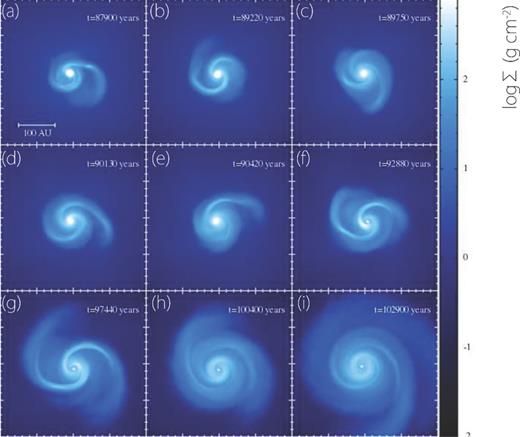
Time sequence for surface density at the cloud centre, viewed face-on for model 1. Elapsed time after the cloud core begins to collapse is shown in each panel.
Fig. 2 shows gas temperatures at the centre of the cloud at the same epochs as in Fig. 1. In comparison with Figs 1 and 2 shows that the structure of the gas temperature is more axisymmetric than that of the surface density. Figs 1 and 2 indicate that there is only a very weak correlation between surface density and temperature. If we assume that the heat source for the disc is viscous heating due to the GI, it is difficult to explain the axisymmetric temperature distribution because gravitational energy is mainly converted to thermal energy around the spiral arms and the heating should be localized around the spiral arms, and thus, the temperature structure should trace the surface density structure. Although we can see weak heating by the spiral arms (e.g. in Fig. 2(g)), the entire temperature structure is almost axisymmetric. Therefore, there must be other heating mechanisms that cause the axisymmetric temperature structure. As we will see below, the radiation flux within the disc determines the axisymmetric component of the gas temperature.
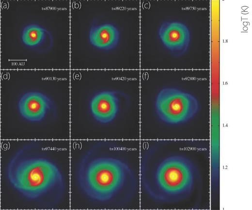
Time sequence for the density-weighted gas temperature at the cloud centre, viewed face-on for model 1. Elapsed time after the cloud core begins to collapse is shown in each panel.
4.1.2 Vertical disc structures
Fig. 3 shows the density contour map on the y = 0 plane at the epoch in Fig. 1(i). The red lines show the scale height of the disc, H(r) = cs, mid(r)/Ω(r), where cs, mid is the velocity of sound on the mid-plane and Ω is the angular velocity at r. The cyan lines show the height of the vertical photosphere zphoto, defined as |$\tau _z=\int ^{\infty }_{z_{\rm photo}} \kappa \rho \mathrm{d}z=1$|. The green lines and arrows show the temperature contour and direction of the radiation flux, respectively. The green lines show that, in the outer region (r ≳ 20 au), the disc is almost vertically isothermal. This feature also occurs in two-dimensional radiation hydrodynamics calculations (Yorke, Bodenheimer & Laughlin 1993). The green arrows around the mid-plane are almost parallel to the x-axis. This indicates that the radial component of the radiation flux dominates the vertical component in the outer disc region. Therefore, the radial component of radiative transfer plays an important role in determining the temperature structure of the disc. We can see weak heating due to the spiral arms at (x, z) = (40 au, 0 au) where the green arrows spread out. Although such spiral heating occasionally occurs, it is transient and does not significantly contribute to the temperature in the outer disc region. Actually, as we will see below, the theoretical disc model in which local heating due to GI balances radiative cooling cannot reproduce the radial profiles of this disc (see thick dashed lines in Fig. 4).
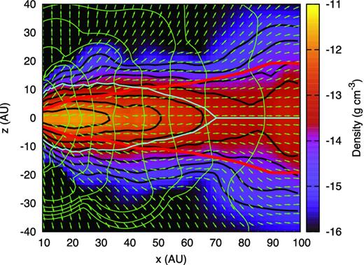
Density contour on the y = 0 plane at the same epoch as in Fig. 1(i) of model 1. Red lines show scale height of disc, H(r); cyan lines show height of vertical photosphere; green lines and arrows show temperature contours and direction of radiation flux, respectively.
The vertical density structure is well described by the vertically isothermal thin disc profile, ρ(z) = ρ0exp (− z2/2H(r)2), although the disc is slightly compressed by the ram pressure of mass accretion from the envelope. The aspect ratio of the disc is about 0.2 at r = 50 au. In the inner region, r ≲ 30 au, the height of the disc photosphere is greater than the disc scale height. This structure is different from a passively irradiated optically thick disc (Kusaka et al. 1970). This is one reason why our discs have a steeper profile T(r) ∝ r−1.1 (see left middle panel in Fig. 4) than the passively irradiated disc model T(r) ∝ r−3/7.
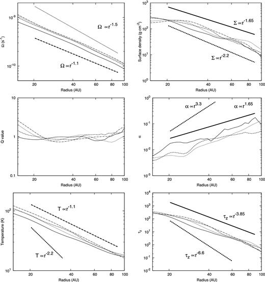
Azimuthally averaged radial profiles of the disc of model 1. Thin solid, dashed, dotted and dashed-dotted lines correspond to profiles at the same epoch as in Figs 1(f), (g), (h) and (i), respectively. Top, middle and bottom left panels show the angular velocity, Toomre's Q value and gas temperature, respectively. Top, middle and bottom right panels show the surface density, α parameter and vertical optical depth, respectively. Thick solid lines show power law profiles estimated from (2), (4), T ∝ r−1.1 and Ω ∝ r−1.1. Thick dashed lines show power law profiles estimated from (2), (4), (11) and Ω ∝ r−1.1. Thick dotted lines show the power law of Kepler rotation Ω ∝ r−3/2. Thick dashed-dotted lines are fittings used for theoretical estimates.
4.1.3 Radial disc structure
Fig. 4 shows the azimuthally averaged radial profiles of the disc. Thin solid, dashed, dotted and dashed-dotted lines are for profiles at the same epochs as in Figs 1(f), (g), (h) and (i), respectively. In the figure, the top left panel shows the angular velocity Ω. Because the disc is massive, the rotation profile is not Keplerian (Ω ∝ r−1.5; thick dotted line). We fitted Ω to Ω ∝ r−1.1 (thick dotted-dashed line) to obtain the power law of the disc with (2) and (4).
The bottom left panel shows the mid-plane gas temperature. The thick dashed line shows the theoretically estimated power law under the assumption that local heating balances local cooling (T ∝ r−2.2). This power law is calculated from (2), (4), (11) and Ω ∝ r−1.1. This power law does not agree with the disc structure because the energy balance is not local, and the radial component of the radiative transfer heats the outer disc region. We fitted the temperature to T ∝ r−1.1 (thick dashed-dotted line). The power law T ∝ r−1.1 can be derived with the diffusion approximation (see Section 4.2.1 for details).
The right top panel shows the profile of surface density Σ. The thick solid lines show the power law that is predicted from (2), (4), Ω ∝ r−1.1 and T ∝ r−1.1. The thick dashed line is the power law predicted from (2), (4), Ω ∝ r−1.1 and (11). In the outer region with r > 20 au, the surface density profile is consistent with the thick solid line. However, in the region r < 20 au, the profile does not agree with the thick solid line because Q is not constant (see left bottom panel), and the assumption of Q ∝ r0 does not apply in this region. The thick-dashed line does not agree with the profile over the entire region.
In the α profile, t0 corresponds to the epochs of Figs 1(f) (solid), (g) (dashed) and (h) (dotted). The profile can be described well by the theoretical estimate from (2), (4), T ∝ r−1.1 and Ω ∝ r−1.1 (α ∝ r1.65; thick solid line). As expected, α was not constant. This is a general feature of a non-isothermal self-gravitating disc. Note that the model in which local viscous heating balances local radiating cooling predicts a very steep radial profile α ∝ r3.3 (thick dashed line) and fails to explain the α profile obtained from the numerical simulation.
The bottom right panel shows the vertical optical depth, τz. The optical depth was calculated from |$\tau _z=\int ^{\infty }_{\infty } \kappa \rho \mathrm{d}z$|. In almost all regions of the disc, the vertical optical depth is greater than unity, τz > 1. Again, the thick solid line describes the radial profile very well.
4.1.4 Cooling time of disc
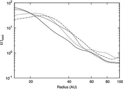
Azimuthally averaged Ωtcool, where tcool is the cooling time of the disc. Thin solid, dashed, dotted and dashed-dotted lines correspond to profiles at the same epoch as in Figs 1(f), (g), (h) and (i), respectively.
4.2 Discussion
4.2.1 Temperature profile determined by radial radiative transfer in an optically thick disc
The results in Section 4.1 shows that the temperature profile of the disc formed in our simulation is T ∝ r−1.1. This is significantly shallower than the disc in which local heating balances local cooling T ∝ r−2.2 (see Fig. 4) and steeper than the passively irradiated disc T ∝ r−3/7. In this subsection, we analytically derive the profile T ∝ r−1.1.
4.2.2 Importance of non-local radiative transfer
As pointed out in Section 1, the locality of radiative cooling has been assumed in many previous simulations (e.g. Rice et al. 2003; Lodato & Rice 2005; Rice, Lodato & Armitage 2005; Paardekooper, Baruteau & Meru 2011; Rice, Forgan & Armitage 2012) and in many analytical studies (Rafikov 2005; Clarke 2009; Kratter & Murray-Clay 2011) to investigate the nature of GI and the conditions of disc fragmentation with radiative cooling. In contrast, our simulations show that radiation can transfer significant energy in the radial direction even in the absence of stellar irradiation.
Consequently, the temperature profile becomes T ∝ r−1.1 in our simulation and is significantly shallower than T ∝ r−2.2, which is expected under the assumption that local viscous heating balances local radiative cooling. Thus, the local energy balance between radiation and viscous heating is not satisfied in the disc formed in our simulations. This indicates that the assumption of local radiative cooling is not necessarily valid in a massive disc around a low-mass star. The radial profiles of the surface density and the viscous α parameter are consistent with a self-gravitating quasi-steady disc model with a given rotation profile and T ∝ r−1.1. Thus, the disc is in the quasi-steady state with an energy balance that is not local.
Therefore, we conclude that the local treatment of radiative cooling is not a suitable approximation to investigate a massive disc around a low-mass star.
We only calculated the disc evolution about 104 yr after protostar formation when the disc and the protostar were still embedded in a massive envelope (class 0 phase). One might think that non-local radiative transfer does not play a role in the later evolutionary phase. However, with a two-dimensional radiation hydrodynamics simulation, Yorke et al. (1993) showed that an almost isothermal temperature distribution in the vertical direction is also realized in the late evolutionary phase of a disc for which 95 per cent of the initial cloud core has already accreted on to the protostar or disc. Thus, we expect that non-local radiative transfer also plays an important role for the temperature structure of discs in the later evolutionary phase. Note that a large simulation box in which the boundary is far from the disc photosphere is crucial for investigating the effects of non-local radiative transfer, otherwise the radiation flux is easily affected by the boundary conditions.
We could not find evidence that the non-local energy transport of GI suggested by Balbus & Papaloizou (1999) plays an important role because GI heating is itself small compared to radiation energy transfer in the outer region of the disc.
4.2.3 Applicability of fragmentation criterion based on disc cooling time
In Fig. 5, we show that the cooling time of the disc corresponds to Ωtcool ≲ 1 in the outer region and our disc apparently satisfies the fragmentation criterion based on the disc cooling time (Q ∼ 1 and Ωtcool ∼ 1). Because the cooling time is very short compared to the orbital period, the gas evolves almost isothermally during the growth of GI in the outer region. However, the disc does not fragment.
For our disc, the most unstable wavelength of the GI is relatively large and global spiral arms develop. The spiral arms readjust the surface density and the disc is stabilized. Such a readjustment was also observed in previous works (Laughlin & Bodenheimer 1994; Kratter et al. 2010). In particular, Kratter et al. (2010) showed that disc fragmentation is suppressed by the readjustment even with an isothermal equation of state. Because such a stabilizing process also plays a role in a realistic disc, we conclude that at least the fragmentation criterion is not a sufficient condition for fragmentation of a realistic disc around a low-mass star.
A significant difference between our disc and discs used in the previous works with a local cooling law is the most unstable wavelength of GI. The discs used in previous studies using a local cooling law (e.g. Rice et al. 2003; Meru & Bate 2012) have a very small value for the most unstable wavelength and the spiral arms formed in these simulations are not geometrically thick and have large azimuthal mode numbers m. It is expected that the efficiency of the readjustment promoted by such spiral arms is small compared to that promoted by global spiral arms that may form in a realistic disc.
Is the fragmentation criterion based on local cooling a necessary condition for disc fragmentation? We think this is not true, either. Although the efficiency of radiative cooling may affect the evolution of condensation formed by GI, a cooling criterion is not necessary for fragmentation of a Q ∼ 1 disc. This can be understood from the previous works that employed the simplified equation of state. For example, Vorobyov & Basu (2006), Inutsuka et al. (2010), Tsukamoto & Machida (2011) and Machida & Matsumoto (2011) employed a barotropic equation of state and the gas evolves adiabatically when ρ ≳ 10−13 g cm−3 (the condensation exceeds this density at a very early phase of its evolution). Even with such a stiff (or adiabatic) equation of state, fragmentation is observed.
Therefore, we conclude that, in general, the fragmentation criterion based on disc cooling time (Q ∼ 1 and Ωtcool ∼ 1) is neither a necessary nor a sufficient condition for fragmentation.
One may think that our results appear very different from the previous results that show that disc fragmentation occurs when the fragmentation criterion is satisfied and does not occur when it is not satisfied (e.g. Rice et al. 2005; Stamatellos & Whitworth 2008, 2009a). However, we emphasize that there is no contradiction. Logically speaking, there are four possible cases:
The disc satisfies (Q ∼ 1 and Ωtcool ∼ 1) and the disc fragments.
The disc does not satisfy (Q ∼ 1 and Ωtcool ∼ 1) and the disc does not fragment.
The disc satisfies (Q ∼ 1 and Ωtcool ∼ 1) but the disc does not fragment.
The disc does not satisfy (Q ∼ 1 and Ωtcool ∼ 1) but the disc fragments.
The previous works mentioned above show examples of cases (i) and (ii). On the other hand, we point out there exist examples of cases (iii) and (iv). Therefore, there is no contradiction.
Note, however, that the finite number of examples of (i) and (ii) are not enough to prove that the disc always fragments when (Q ∼ 1 and Ωtcool ∼ 1) is satisfied or that the fragmenting disc must always satisfy (Q ∼ 1 and Ωtcool ∼ 1), because we cannot prove the non-existence of exceptions with a finite number of simulations. On the other hand, just one counter-example is enough to reject these statements. In this paper, we show there exists an example of case (iii) and this is a counter-example for the statement, the disk always fragmenting when (Q ∼ 1 and Ωtcool ∼ 1) is satisfied. Therefore, the fragmentation criterion is not a sufficient condition. On the other hand, the previous works we mentioned above show that there exists an example of case (iv). This is a counter-example for the statement, the fragmenting disc must always satisfy (Q ∼ 1 and Ωtcool ∼ 1). Therefore, the fragmentation criterion is not a necessary condition. Here we emphasize that the discussions above is based on azimuthally averaged quantities (see Section 5.1.2).
4.2.4 Resolution consideration for disc fragmentation simulations
Resolution consideration of the simulations performed in this paper
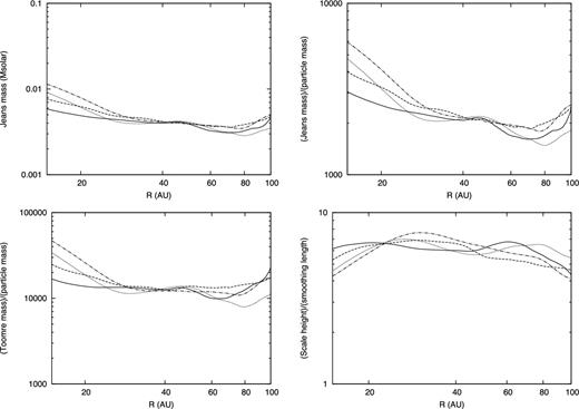
Azimuthally averaged Jeans mass (top left), ratio of Jeans mass to SPH particle mass (top right), ratio of Toomre mass to SPH particle mass (bottom left) and ratio of scale height to smoothing length (bottom right). Each line corresponds to the same epoch as in Figs 1(f) (solid), (g) (dashed), (h) (dotted) and (i) (dashed-dotted).
The Jeans mass of our disc is about 4 × 10⁻³ M⊙ over almost the entire region of the disc; this value is consistent with the initial clump mass that formed in model 2. As shown in the top right panel, the Jeans mass is resolved by more than ∼2000 particles. In our simulations, we adopted the number of neighbours to be Nn ∼ 50; hence, the mass resolution is about 20 times higher than that required by Bate & Burkert (1997).
The Toomre mass is resolved by more than ∼10 000 particles and this is about 30 times higher than the resolution criterion suggested by Nelson (2006). The bottom right panel shows that the vertical scale height H is resolved by larger than 4hsml and our simulation also satisfies the resolution requirement for vertical scale height. Therefore, we conclude that the numerical resolution in our simulation was sufficient to resolve fragmentation of the disc.
Resolution consideration of the simulations with a local cooling law
Why does the disc fragmentation criterion with a local cooling law strongly depend on the numerical resolution? To answer this question, we investigate the resolution requirement of the disc used in Rice et al. (2005) and Meru & Bate (2012) with the quasi-steady state structure. In Section 2, we investigated the steady state of a self-gravitating disc with a local cooling law. As we pointed out, the temperatures of the discs used in Rice et al. (2005) and Meru & Bate (2012) are very small in the quasi-steady state. Therefore, we can expect that the requirement for the numerical resolution for their discs that settled into quasi-steady states is very severe. In this subsection, we only consider the resolution requirement suggested by Bate & Burkert (1997).
In Fig. 7, we show the Jeans mass (top) and the required particle number to resolve the Jeans mass Nreq = 2NnMdisc/MJeans (bottom) as functions of the radius for a disc that has dimensionless parameters of Mstar = 1, Mdisc = 0.1, rin = 0.25 and rout = 25, and is in the quasi-steady state Σ ∝ r−3/2, T ∝ r0 and α ∝ r0. Here according to Rice et al. (2012), we approximated MJeans = πΣH2 for comparison and we assumed Nn = 50. The Jeans mass MJeans ≲ 10−5. This corresponds to about 0.01MJupiter if we regard the central star mass as 1 M⊙. This value of the Jeans mass is very small compared to that in our simulation and to the mass of wide-orbit planets (∼10MJupiter).
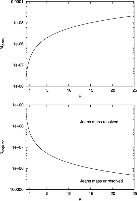
Jeans mass (top) and required number of particles to resolve the Jeans mass, Nreq = 2NnMdisc/MJeans (bottom) for a disc in which Mstar = 1, Mdisc = 0.1, rin = 0.25 and rout = 25 are adopted with the disc in the quasi-steady state with the local cooling law (8).
The bottom panel in Fig. 7 shows that a particle number of Np ≳ 107 is required to resolve the Jeans mass. Note that with Np < 500 000, the Jeans mass is not resolved over the entire disc region. Meru & Bate (2012) showed that the convergence of the calculation around Np ≳ 107 and their results are consistent with our estimate. Our estimate is more severe than that of Rice et al. (2012) in the outer disc region. The difference is because Rice et al. (2012) assumed Σ ∝ r−1 instead of assuming the steady state as in (2). Therefore, they derived T ∝ r1/2 and found a larger MJeans in the outer disc region. Note, however, that such a disc is not realized with a local cooling law because the surface density profile also changes because of the angular momentum transfer to realize the quasi-steady state structure (see fig. 1 of Baruteau et al. 2011).
In an isolated disc with a local cooling law and without a temperature floor, the disc cools infinitely to maintain Q = 1, and the Jeans mass becomes infinitely small as the disc evolves (or as the surface density decreases). We must carefully monitor the Jeans mass during the simulations.
On the other hand, in a realistic system, there exists an appropriate range of temperature or of the Jeans mass, depending on the system of interest. We emphasize that the nature of the GI depends not only on the value of Q but also on the most unstable wavelength of GI, |$\lambda _Q={2 c_s^2}/{G \Sigma }$| (|${\sim } \lambda _{\rm Jeans}^2/H$|), and different length scales give strikingly different outcomes for the non-linear growth phase. For example, the widths of spiral arms and masses of fragments differ for different length scales (compare the spiral pattern in Fig. 1 with fig. 1 in Rice et al. 2005).
We suggest that future self-gravitating disc simulations should use a disc model that has a realistic Jeans length. For example, the irradiated disc model (e.g. Cai et al. 2008) or a locally isothermal model seems to be more suitable for numerical simulations because we can limit the value of the most unstable wavelength to a realistic range. To construct appropriate initial conditions, the profiles derived in Section 2 would be useful.
5 DISC FRAGMENTATION AND EVOLUTION OF CLUMPS
In this section, we investigate fragmentation of a disc and the evolution of clumps after their formation. Understanding the evolution of a clump is crucial for the possible final outcomes (wide-orbit planets, brown dwarfs or binary/multiple systems) that could result from disc fragmentation.
5.1 Simulation results
5.1.1 Parameter survey for disc fragmentation
As shown in Table 1, we calculated the evolution of the cloud core for five models. In models 1, 3 and 5, fragmentation did not occur in the early phase of disc evolution. On the other hand, in models 2, 4 and TMI13, fragmentation did take place. The computation results are summarized in Fig. 8. In that figure, circles (triangles) indicate models in which fragmentation did not (did) occur. The figure shows how fragmentation correlates with |$\dot{M}$|, the mass accretion rate on to the disc, and rcent, the centrifugal radius of the fluid element. Qualitatively, larger mass accretion rates and larger centrifugal radii lead to fragmentation. The boundary that divides the fragmentation and no-fragmentation models is consistent with that determined by simulations with the barotropic approximation (see Tsukamoto & Machida 2011). This result suggests that, in the early evolution of a disc, fragmentation rarely depends on radiative transfer or the thermodynamics of the gas. This is because disc fragmentation in the early evolutionary phase is mainly determined by the mass accretion rate on to the disc and the angular momentum of mass accretion (Matsumoto & Hanawa 2003; Saigo & Tomisaka 2006; Vorobyov & Basu 2010a,b; Inutsuka et al. 2010; Tsukamoto & Machida 2011).
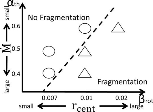
Classification of simulation results on the αth–βrot plane. Circles and triangles denote no-fragmentation and fragmentation models, respectively. The dashed line shows the boundary between fragmentation and no fragmentation.
5.1.2 Differences in the conditions between fragmenting and non-fragmenting discs
In this subsection, we investigate the differences in the conditions between fragmenting and non-fragmenting discs. In Fig. 9, we show the Q value and cooling time of models 1 (red lines; non-fragmenting disc) and 2 (green lines; fragmenting disc). The epoch of the red lines is the same as in Fig. 1(h). The epoch of the green lines is the same as in Fig. 10(a) and just prior to disc fragmentation. The solid lines of Fig. 9 show the azimuthally averaged Q value and the azimuthally averaged cooling time normalized by orbital period. They show both discs are gravitationally unstable (Qave ∼ 1) and their cooling time is sufficiently small ((Ωtcool)ave ∼ 1). From the azimuthally averaged quantities, we cannot find any significant difference between two the discs. But one fragments and the other does not. What is the difference between them?
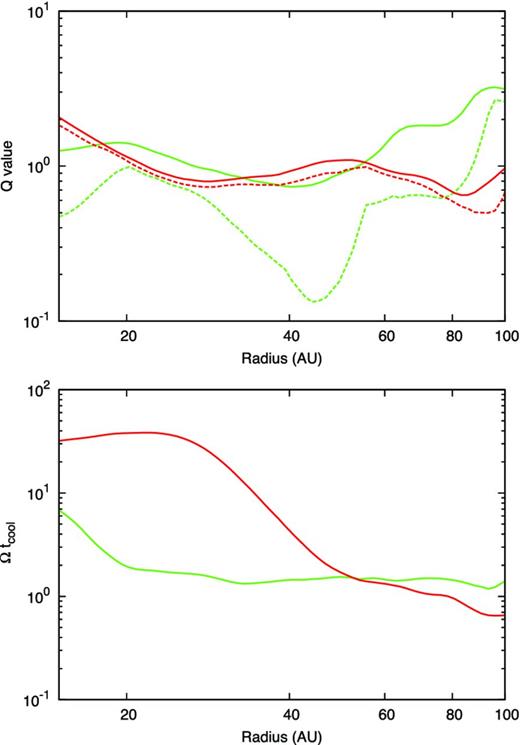
Top panel shows the azimuthally averaged Q values Qave (solid) and minimum Q values Qmin (dashed) for non-fragmenting (red; model 1) and fragmenting discs (green; model 2). Bottom panel shows the azimuthally averaged Ωtcool of non-fragmenting (red) and fragmenting discs (green). The epoch of the red lines is the same as in Fig. 1(h). The epoch of the green lines is the same as in Fig. 10(a) and just prior to disc fragmentation.
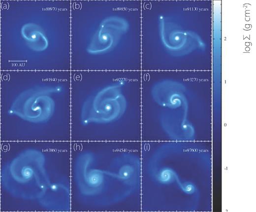
Time sequence for surface density at the cloud centre, viewed face-on for model 2. The elapsed time after the cloud core begins to collapse is shown in each panel.
The dashed lines in Fig. 9 show the minimum Q value Qmin at each radius. This traces the Q value at the spiral arms. We can see a clear difference between the red and green dashed lines. The Qmin of the fragmenting disc becomes significantly small (Qmin ≲ 0.2) for a relatively large width (Δr ∼ 10 au). On the other hand, the profile of Qmin for a non-fragmenting disc does not show such a dip. We monitored Qmin during the entire period of evolution of the non-fragmenting disc after protostar formation and found that Qmin < 0.2 is never satisfied. Note also that the width of the spiral arms of the fragmenting disc is smaller than that of the non-fragmenting disc [compare Fig. 1(h) with Fig. 10(a)].
From these results, we conclude that the Q value inside the spiral arms (not the azimuthally averaged Q value) and the width of the spiral arms are important quantities for disc fragmentation. The importance of the width of the spiral arms was also pointed out by Rogers & Wadsley (2012).
5.1.3 Fragmentation of discs and evolution of the clumps
In this subsection, we consider the evolution of the fragments (or clumps) formed by disc fragmentation. We have already investigated the evolution of clumps (Tsukamoto et al. 2013b). The parameters for the cloud core investigated in Tsukamoto et al. (2013b) were αth = 0.3844 and βrot = 0.01 (model TMI13 in Table 1). In model TMI13, low αth and βrot were adopted, which means that the disc formed is compact. In that case, fragmentation occurred in the region T ≳ 20 K. Thus, the entropy of the the centres of the clumps is greater than that of the typical first core (see fig. 4 in Tsukamoto et al. 2013b).
When the initial cloud core has a high value of βrot, it is expected that the disc will be more outspread, and clumps will form in low-temperature regions. Therefore, the entropy of the clumps would become small. The central entropy of clumps is important when we consider the initial mass and evolution of clumps. Smaller entropy leads to smaller clump mass (see equation (35)) and a smaller clump radius. Thus, investigating clump evolution for larger values of αth and βrot would be insightful to understand the initial properties and the evolutionary process of clumps in more detail. To do so, we investigate clump evolution in model 2. The cloud core of model 2 has αth and βrot values greater than those in model TMI13.
Fig. 10 shows the evolution of surface density at the centre of the cloud core for model 2. Analogous to Figs 1 and 10(a) shows a bimodal structure (the first core and disc around it) in the early phase of disc evolution. The first clump formed in Fig. 10(b). We define the epoch of clump formation as the time when the central density exceeds 10−11 g cm−3. Within 8000 yr after the first clump formed, six more clumps formed.
Fig. 11 shows the temperature evolution at the centre of the cloud core of model 2. As expected, disc fragmentation and clump formation occur in the very low-temperature region T ∼ 10 K. After disc fragmentation, the central temperature of the clump quickly increases because of compressional heating.
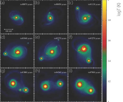
Time sequence for the density-weighted gas temperature at the cloud centre, viewed face-on for model 2. The elapsed time after the cloud core begins to collapse is shown in each panel.
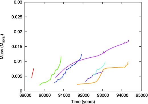
Fig. 12 shows the orbits of clumps after clump formation (solid lines) and the fluid elements at the centres of the clumps prior to clump formation (dashed lines). Four clumps, shown with red, green, blue and cyan lines, finally accreted on to the central first core or protostar. On the other hand, the remaining three clumps, shown with magenta, purple and orange lines, merged into one clump and became a secondary protostar [see Fig. 10(i)].
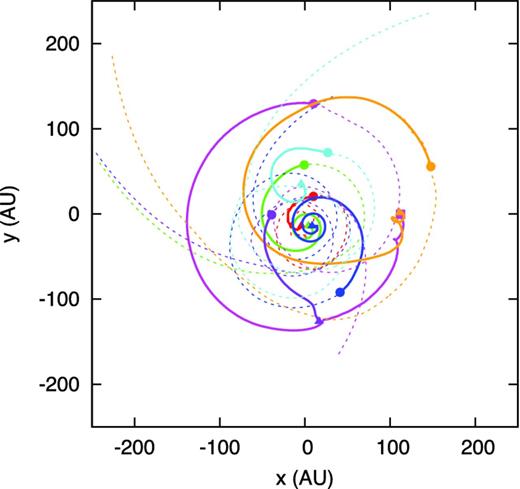
Orbits of clumps (solid lines). Dashed lines represent orbits of the fluid elements of the clump centre before clump formation (ρc < 10−11 g cm−3). Symbols mark positions where clumps form (circles), the clump central density begins to decrease or the clump begins to be destroyed (triangles), and second collapse begins in the clump or the sink particles are inserted (square).
Fig. 13 shows the temperature evolution of the centres of the clumps as a function of density (solid lines). The figure also shows the temperature evolution of fluid elements at the centres of the clumps prior to clump formation (dashed lines). In this figure, a typical temperature evolution with the barotropic equation of state, which is designed to mimic the temperature evolution of the centre of the first core (Masunaga & Inutsuka 2000), is also shown for comparison.
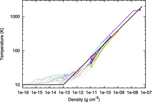
Temperature at the centres of clumps (solid lines) as a function of density. Dashed lines represent the temperature evolution of fluid elements at clump centres before clump formation (ρc < 10−11 g cm−3). Symbols and colours are the same as in Fig. 12. A typical evolution for the barotropic approximation is shown by the black solid line.
Until the density reaches ∼10−13 g cm−3, the temperature is almost isothermal because there is no significant heating by spiral arms. On the other hand, above ∼10−13 g cm−3, the gas evolution becomes adiabatic. The interesting finding is that the thermal evolution of the central temperature is almost consistent with the evolution in the barotropic approximation (black solid line). Because clumps form in the disc, we might expect that fluid elements at the centres of clumps have a good chance of decreasing their entropy by radiative cooling compared with that of the first core, which is surrounded by a spherically symmetric massive envelope. However, our results show that the centres of clumps do not efficiently cool before they become optically thick. As a result, the evolution of fluid elements follows the line of the barotropic equation of state.
For the magenta clump, the second collapse occurred about 3000 yr after its formation. This timescale is consistent with our previous results (Tsukamoto et al. 2013b). Note that the second collapse occurs at a slightly smaller mass (∼0.015 M⊙) compared to that in our previous results. This is because the central entropy of the clump is smaller than that of the clumps in Tsukamoto et al. (2013b). The smaller central entropy induces the second collapse at a smaller clump mass [see (3) in Tsukamoto et al. 2013b].
5.2 Discussion
5.2.1 Minimum central entropy of clumps
An important finding in Section 5.1.3 is that the evolutionary paths of the central temperatures of clumps on the ρ–T plane are close to that of the first core even though the clumps form in the disc. This implies that clump evolution after the fragmentation can be approximately regarded as spherically symmetric. Therefore, in the same manner as for the first core, we can describe the evolution of the central entropy of the clump.
Note that the minimum entropy does not depend on κ0 when the ratio of heat capacities γ is equal to 7/5 because |$T_{\rm ad}/\rho _{\rm ad}^{\gamma -1} \propto \kappa _0^{3/2(\gamma - 7/5)}$| (Omukai et al. 2005). Therefore, the evolution of the central region of the clump follows the same track in the ρ–T plane irrespective of different κ. The property is the same as in the evolution of the protostars with various metallicities shown by Omukai et al. (2005).
5.2.2 Minimum initial mass of the clump
5.2.3 Comparison with previous work
There have been few studies on the evolution of clumps with realistic accretion on to them and sufficient numerical resolution to resolve the central structure of the clump (Stamatellos & Whitworth 2009b; Tsukamoto et al. 2013b). In this subsection, we compare our results with those in Stamatellos & Whitworth (2009b).
Stamatellos & Whitworth (2009b) investigated the evolution of clumps with a three-dimensional simulation starting from a massive isolated disc. In the disc, fragmentation immediately occurs and the clumps form. They showed that a clump undergoes a second collapse when its mass reaches ∼10MJupiter and the timescale for the second collapse is several thousand years. They also point out that thermal evolution of the clump is consistent with the evolution of the first core (Masunaga & Inutsuka 2000). The evolution of the clumps formed in our simulation is consistent with that found in their simulations.
However, there are interesting differences between their results and ours. In their simulations, most of the clumps remained in the disc without falling on to the central protostar. On the other hand, in our simulation, a large fraction of clumps fell on to the central star and disappeared. This difference may arise because the initial disc of Stamatellos & Whitworth (2009b) is very massive (0.7 M⊙) and unstable (Q ∼ 0.9). In such a massive disc, fragmentation immediately occurs and many clumps simultaneously form. Thus, many clumps reside in the disc at the same epoch and interact with each other. On the other hand, in our simulation, only two or three clumps simultaneously exist in the disc at the same epoch because the disc is not so massive. The difference in the orbital evolution of the clumps may come from the difference between the discs. The orbital evolution of clumps depends very strongly on the condition of the disc, and further studies are needed on this issue.
5.2.4 Possible evolutionary path to realize a small-mass clump
Our simulation results have shown that the central entropy of a clump cannot become significantly smaller than that of the first core. However, there is a possible path that can lead to a clump with a central entropy smaller than that of the first core. The above discussion relies on clump evolution after disc fragmentation. Thus, the value of Q in the disc has already become Q ∼ 1. Once GI turns on, the surface density decreases by mass and angular momentum transfer by the spiral arms, or disc fragmentation occurs. As shown in Section 5.1.3, the rapid evolution of a clump after fragmentation prevents temperature evolution, which leads to a smaller central entropy than that of the first core.
This indicates that a high mid-plane density can be achieved in the inner region of the disc. If a disc with such a high mid-plane density at the inner region and low temperature somehow fragments, a clump with small central entropy could be created. For example, if a disc with a temperature of 50 K at 10 au around 1 M⊙ fragments, adiabatic contraction of the clump begins from ρ ∼ 10−10 g cm−3 and T = 50 K. In such a case, the initial mass of the clump is ∼0.7MJupiter. However, the realization of such a disc seems to require a magnetic field (Inutsuka et al. 2010; Machida et al. 2011), which is beyond the scope of this paper.
6 SUMMARY AND FUTURE STUDY
6.1 Summary
In this paper, we investigate the structure of self-gravitating discs, their fragmentation and the evolution of the fragments using an analytic approach and three-dimensional radiation hydrodynamics simulations. First, we analytically derive the quasi-steady structures of self-gravitating discs with various energy equations. We show that a local cooling law, which has been widely used in previous studies (e.g. Lodato & Rice 2005; Rice et al. 2005; Paardekooper et al. 2011; Meru & Bate 2012), describes a globally isothermal disc (T ∝ r0) in the quasi-steady state. In addition, we point out that the Jeans mass of a disc with a local cooling law and the fiducial disc model (Mstar = 1, Mdisc = 0.1, rin = 0.25 and rout = 25) becomes very small and the resolution requirement for the simulation is exceedingly severe. We show that at least ∼107 particles are required to resolve the Jeans mass of the disc. We also point out that such a small Jeans mass (∼10−5 M⊙, if we regard the mass of the central star as 1 M⊙) is not attainable in a realistic disc around a low-mass star since it requires an unrealistically low temperature.
We also investigated the quasi-steady structure of a disc in which radiative cooling locally balances viscous heating and showed that it has very steep radial profiles (e.g. T ∝ r−3 for a Keplerian disc) in the quasi-steady state. To investigate whether such a steep profile can be realized (in other words, whether the local balance between radiative cooling and viscous heating can be realized), we conducted three-dimensional radiation hydrodynamics simulations. We found that the disc does not have the radial profile expected from the local energy balance and that the disc temperature is non-locally determined by radiative transfer. The radial profile of the disc temperature was T ∝ r−1.1 and this scaling can be derived analytically by applying a diffusion approximation. Because the temperature of the disc is determined by radial radiative transfer within the disc, radial radiation transport is crucial for the outer regions of the disc. Thus, we conclude that a description with only local radiative cooling is not viable for massive discs around low-mass stars.
The disc formed in our simulation satisfies the fragmentation criterion based on disc cooling time (Q ∼ 1 and Ωtcool ∼ 1). However, fragmentation was not observed in the disc. Therefore, the fragmentation criterion is not a sufficient condition for fragmentation. Further studies to produce a more accurate criterion are needed.
Mass accretion from the envelope is another process that possibly drives disc fragmentation. Using a parameter survey with radiation hydrodynamics simulations starting from the molecular cloud core, we determined the parameter range of the host cloud core needed for gravitational fragmentation. The parameter range is in agreement with that obtained in our previous study based on a simplified equation of state (Tsukamoto & Machida 2011). Therefore, we conclude that a detailed treatment of radiative transfer is not crucial for disc fragmentation driven by mass accretion from the envelope.
We also investigated the internal evolution of fragments (clumps) formed in extended cold discs (T ∼ 10 K in the outer region). Even in such a disc, the central temperature of a clump does not fall sufficiently to give a smaller central entropy than that of the first core. Therefore, there is a minimum value of the central entropy. Using this value for the central entropy, we derived the minimum initial mass of the clumps to be about a few Jupiter masses. This is consistent with the initial mass formed in our simulations.
6.2 Future study
In our simulations, the FLD approximation was adopted. It is well known that the FLD approximation does not behave well in an optically thin region. Although the disc formed in our simulation can be regarded as optically thick in almost all regions, it is possible that the temperature profile is different for more realistic radiative transfer methods because the simulation box includes the optically thin region and the radiation flows along a roundabout path in the FLD approximation. Although the difference is expected to be approximately a small factor (see comparison tests of radiative transfer schemes, e.g. Pascucci et al. 2004; Kuiper & Klessen 2013), it is important to perform simulations with a more sophisticated radiative transfer method. We plan to do so to confirm our results for the disc structure of a massive disc around a low-mass star.
Another important issue, which is not discussed in this paper, is the effect of magnetic fields. These play important roles in the formation and early evolution of circum-stellar discs due to their efficient transfer of angular momentum and the formation of outflows (see Inutsuka 2012, and references therein). In particular, magnetic fields would change the parameter range of fragmentation that is derived in Section 5.1.1. They could also be important for the orbital and internal evolution of clumps. A disc is well coupled to the magnetic fields because magnetic diffusion is not significant in the range of disc densities. On the other hand, magnetic diffusion is effective inside clumps because of their high density. Thus, the magnetic field and clumps would be decoupled. In our future study, we will investigate the effects of magnetic fields using numerical methods for smoothed particle magneto-hydrodynamics as described in Iwasaki & Inutsuka (2011) and Tsukamoto, Iwasaki & Inutsuka (2013a).
We thank K. Iwasaki, T. Matsumoto, H. Kobayashi, M. Ogihara, K. Tanaka and T. Muto for fruitful discussions. We also thank K. Tomida and Y. Hori for providing their equation of state (EOS) table. We also thank the referee, Dr D. Stamatellos, for insightful comments. The snapshots were produced by SPLASH (Price 2007). The computations were performed on a parallel computer, an XC30 system at center for computational astrophysics (CfCA) of national astronomical observatory of Japan (NAOJ) and an SR16000 at Yukawa institute for theoretical physics (YITP) in Kyoto University. YT is financially supported by a Japan society for the promotion of science (JSPS) research fellowship for young scientists.
