


ABSTRACT
We observed the Ultraluminous X-ray Source (ULX) IC 342 X-1 simultaneously in X-ray and radio with Chandra and the JVLA to investigate previously reported unresolved radio emission coincident with the ULX. The Chandra data reveal a spectrum that is much softer than observed previously and is well modelled by a thermal accretion disc spectrum. No significant radio emission above the rms noise level was observed within the region of the ULX, consistent with the interpretation as a thermal state though other states cannot be entirely ruled out with the current data. We estimate the mass of the black hole using the modelled inner disc temperature to be |$30 \,\mathrm{M_{{\odot }}} \lesssim M\sqrt{\mathrm{cos}i}\lesssim 200 \,\mathrm{M_{{\odot }}}$| based on a Shakura–Sunyaev disc model. Through a study of the hardness and high-energy curvature of available X-ray observations, we find that the accretion state of X-1 is not determined by luminosity alone.
1 INTRODUCTION
Ultraluminous X-ray sources (ULXs) are non-nuclear, extragalactic accreting compact objects whose X-ray luminosities exceed the Eddington limit for stellar mass black hole binaries (BHB) with mass ≲20 Mȯ. Their high luminosities suggest they are either intermediate-mass black holes (IMBH) (Colbert & Mushotzky 1999; Makishima et al. 2000; Kaaret et al. 2001), that their emission is beamed (e.g. Poutanen et al. 2007; King 2009), or that they are stellar-mass BHBs that are emitting at super-Eddington rates (e.g. Begelman 2002). Beaming alone cannot account for the excess luminosity from all sources, as demonstrated by observations using He ii recombination lines in surrounding nebula for the ULX Holmberg II X-1 and for NGC 5408 X-1 showing the observed luminosity to be consistent with relatively isotropic emission (Pakull & Mirioni 2003; Kaaret, Ward & Zezas 2004; Kaaret & Corbel 2009). Likely the ULX population is explained by some combination of these models. By studying the unique characteristics and spectral evolution of ULXs, and comparing their spectral and timing features to the well known properties of BHBs, we can hope to elucidate the physical processes that drive these sources.
Spectral curvature above ∼6 keV in the hard component of a large fraction of ULX spectra (Stobbart, Roberts & Wilms 2006; Gladstone, Roberts & Done 2009; Miyawaki et al. 2009) distinguishes them from BHBs, whose hard component is generally modelled by a power law which extends unbroken to much higher energies, often above ∼100 keV. With sensitivity above 10 keV, recent observations with the Nuclear Spectroscopic Telescope Array (NuStar) have confirmed a spectral cutoff in ULXs such as NGC 1313 X-1 (Bachetti et al. 2013). Gladstone et al. (2009) suggested that the high-energy roll-over and soft spectral feature seen in many ULX spectra may correspond to a super-Eddington state of accretion on to a stellar-mass BH (the ‘ultraluminous’ state). The spectral curvature is thought to be due to heavy Comptonization of disc photons by a cool, optically thick corona. Further study of ULX populations has motivated the classification of three distinct ULX states: a Broadened disc state, and two-component hard ultraluminous and soft ultraluminous states (Sutton, Roberts & Middleton 2013). The broadened disc state is thought to occur near the Eddington accretion rate, while the latter two likely represent super-Eddington accretion states.
For a single source, transitions between accretion states in the ultraluminous classification scheme are ascribed solely to changes in the accretion rate. Inclination is also expected to affect the state classification (Poutanen et al. 2007; Sutton et al. 2013), but would not change over time for a single source with a fixed orientation to the observer. Luminosity is often used as a predictor of accretion rate, and in BHBs it is well established that the spectral state is not set by the luminosity alone (for a review, see Remillard & McClintock 2006). Grisé et al. (2010) and Vierdayanti et al. (2010) have shown that the spectral state varies at a single luminosity for the ULXs Holmberg II X-1 and Holmberg IX X-1, respectively, suggesting that an additional parameter beyond accretion rate can vary for individual sources. It would be interesting to discover whether this trait is common to other ULXs and, thus, an additional parameter is needed to set the accretion state of a given source.
IC 342 is a nearby (3.9 Mpc; Tikhonov & Galazutdinova 2010) starburst galaxy that contains two ULXs, X-1 and X-2. X-1 is surrounded by a large optical and radio nebula that may be an X-ray ionized bubble driven by strong outflows from the ULX (Pakull & Mirioni 2003; Roberts et al. 2003; Feng & Kaaret 2008). X-1 and X-2 were the first ULXs reported to transition between distinct spectral states (Kubota et al. 2001). X-1 transitioned from an apparently disc-dominant state to a power-law-dominant state while the spectrum of X-2 coincidentally made the reverse transition.
The X-ray spectrum of IC 342 X-1, hereafter X-1, has previously been observed in a spectral state characterized by a high luminosity, apparently cool disc, and a spectral turnover at high energy (Feng & Kaaret 2009; Yoshida et al. 2013). Feng & Kaaret (2009) reported an anti-correlation between the X-ray luminosity and temperature of the soft energy feature of X-1, ruling out interpretation of the soft component as thin disc emission. A negative temperature–luminosity correlation is predicted if the soft component is caused by optically thick outflows thought to occur in a super-Eddington accretion state (Poutanen et al. 2007; Kajava & Poutanen 2009). Therefore, X-1 is a strong candidate for a source which enters super-Eddington or ‘ultraluminous’ accretion states.
In VLA observations of X-1 in 2007 and 2008, Cseh et al. (2011, 2012) reported possible unresolved radio emission coincident with the ULX which was not detected with follow-up EVN observations. To confirm or deny the existence of a self-absorbed compact jet and investigate whether a relationship known as the Fundamental Plane (FP) of black hole activity (Merloni, Heinz & di Matteo 2003; Falcke, Körding & Markoff 2004) could be used to estimate the mass of the BH, we obtained simultaneous radio and X-ray observations of X-1.
In this paper, we describe the spectral properties of the recent Chandra X-ray and JVLA radio observations of X-1. We also analyse previous high-quality X-ray observations of the source in a systematic fashion to investigate the evolution of the system over time via its X-ray intensity, spectral hardness, and high-energy curvature. We additionally estimate the mass of the BH using fit parameters from the most recent Chandra observation.
2 X-RAY OBSERVATIONS AND REDUCTION
We analysed a new Chandra observation of X-1 and completed the analysis of the previous high-quality observations of X-1 in order to examine the evolution of its spectral properties. The data were reduced using heasoft (version 6.13) with up-to-date calibration files as of 2013 May. Reduction and analysis details for each instrument are described in this section.
The observations, with references to previous analysis in the literature and observation identifiers used in this paper, are summarized in Table 1. We have chosen to include Chandra observations described by Roberts et al. (2004) only in the hardness–intensity diagram (HID) due to pileup concerns. Using the xspec tool pileup map, we find that these observations have maximum count rates per frame of >0.14 in the region of X-1, corresponding to a pileup fraction greater than 5 per cent. We exclude all available Swift observations because they have too few counts to confidently constrain the spectral properties.
Summary of observations.
| Identifier | Date | Instrument | Exposure | Counts | ObsID | Ref |
|---|---|---|---|---|---|---|
| (1) | (2) | (3) | (4) | (5) | (6) | (7) |
| ASCA1 | 19/09/1993 | ASCA | 77.7 | 16621 | 60003000 | A, B, C, D, E |
| ASCA2 | 24/02/2000 | ASCA | 545 | 15804 | 68001000 | C, D, E |
| XM1 | 11/02/2001 | XMM–Newton | 9.5 | 3932 | 0093640901 | F, G, I, J, K, L |
| XM2 | 20/02/2004 | XMM–Newton | 21.2 | 22962 | 0206890101 | G, I, J, L |
| XM3 | 17/08/2004 | XMM–Newton | 23.4 | 13026 | 0206890201 | G, H, I, J, L |
| XM4 | 10/02/2005 | XMM–Newton | 7.6 | 12943 | 0206890401 | G, I, J, L |
| SU1 | 07/08/2010 | Suzaku | 74.4 | 22059 | 705009010 | J |
| SU2 | 20/03/2011 | Suzaku | 75.5 | 23408 | 705009020 | J |
| CHR | 26/08/2002 | Chandra | 9.9 | 2313 | 2917 | J |
| CH | 29/10/2012 | Chandra | 9.1 | 2245 | 13686 | This Paper |
(1) Identifiers follow convention of Yoshida et al. (2013); (2) Date of observation; (3) Instrument; (4) Duration of observation after filtering (ks); (5) Total counts in spectrum included in fitting; (6) Observation ID; (7) Selected reference to previous analysis in literature.
(A) Okada et al. (1998); (B) Makishima et al. (2000); (C) Mizuno, Kubota & Makishima (2001); (D) Watarai, Mizuno & Mineshige (2001); (E) Kubota et al. (2001); (F) Wang et al. (2004); (G) Feng & Kaaret (2009); (H) Gladstone et al. (2009); (I) Mak, Pun & Kong (2011); (J) Yoshida et al. (2013); (K) Sutton et al. (2013); (L) Pintore et al. (2014).
2.1 New Chandra observations
X-1 was observed with Chandra's Advanced CCD Imaging Spectrometer (ACIS) for 9.13 ks in its FAINT mode on 2012 October 29 beginning at 07:10:25 UTC (ObsId 13686), coincident with the JVLA radio observations. X-1 is a bright source with an ACIS counting rate ∼0.2 c s−1 and has suffered from pileup in previous Chandra observations. To avoid pileup, the observations were carried out using offset pointing (3.43 arcmin), operating only the S3 chip and using a 1/8 sub-array to reduce the frame time to 0.4 s. Data reduction was performed using the Chandra Interactive Analysis of Observation software package (ciao) (data processing version 8.4.5, caldb version 4.5.2), beginning with the level 2 event files. dmextract was used to create a light curve of the events on the S3 chip to look for background flares. No flares were observed and the maximum count rate was below 2.5 counts per second.
Offset pointing increases the positional uncertainty approximately to 1/4 times the 50 per cent encircled energy radius at the offset position.1 For our 3.43 arcmin offset and a photon energy of 5 keV, we used the ciao utility mkpsfmap to find the encircled energy radius and determined a positional uncertainty of 0.33 arcsec. The ciao wavdetect utility was used to search for point sources in the field using a significance threshold of 10−6 and returned four sources. The ULX is identified with a source centred at R.A. = |$3^{\rm h}45^{\rm m}55{^{\rm s}_{.}}55$|, Dec. = +68°04′55|${^{\prime\prime}_{.}}$|25 (J2000.0), consistent with the previously determined location of the ULX by Feng & Kaaret (2008) within positional uncertainties.
The ciao specextract utility was used to extract a spectrum and create unweighted, point-source aperture corrected ARF and RMF response matrices for events on the S3 chip using a 4 arcsec circular region centred at R.A. = 3:45:55.594, Dec. = +68:04:55.39, enclosing ∼90 per cent of the PSF at 8 keV. The background is specified by a surrounding annular region with an inner radius of 15.17 arcsec and outer radius of 28.7 arcsec. xspec version 12.8.0 (Arnaud 1996) was used to fit the spectrum in the 0.7–8 keV band. Events were grouped to 15 counts per bin.
2.2 ASCA
We screened event files for two ASCA observations using the heasoft ascascreen tool with standard REV2 screening procedures. A circular region of 3 arcmin radius was used to extract the spectrum of X-1 in both of the ASCA observations, encircling more than 60 per cent of the energy at 4.5 keV (SIS) and avoiding overlap with IC 342 X-2. There are three additional X-ray sources which overlap this region, sources 6, 12 and 9 which are described by Kong (2003). We mask out sources 6 and 12 using circular regions of 77 arcsec radius. Source 9 is unresolved by ASCA, but is not expected to cause significant contamination as its flux is approximately 1/10 that of X-1 in the 0.2–12 keV band (and only 4 per cent for the brighter ASCA1 observation). The luminosity of source 9 also appears constant over several years within errors (Kong 2003; Mak, Pun & Kong 2008). The inferred fluxes do not depend on the extraction region size as corrections for encircled energy fraction are included in the response files. The heasarc Ftools interface, xselect, was used to extract spectra for both GIS and SIS instruments. An energy range of 0.7–10 keV was used to fit the spectra due to the cutoff in instrumental sensitivity outside of this range.
Both the SIS and GIS instruments were analysed from the 1993 ASCA (ASCA1) observation. Because the source falls across two chips of the SIS detector, the response files were created for the source taking into account the gap between chips. sisrmg was used to create the SIS response matrices for each side of the gap, which were combined using addrmf with weighting by total counts within the source region on each CCD chip. SIS0 and SIS1 spectra were combined using addascaspec for bright and bright2 mode data separately. The SIS and GIS spectra were fit simultaneously, and a constant multiplier was fit in front of the GIS spectrum to account for its lower response compared to the SIS instrument; the constant was found to range between 1.1 and 1.15. Background files were created for the GIS using blank sky data with the tool mkgisbgd, and the GIS2 and GIS3 spectra and ancillary response file (arf) were combined using the tool addascaspec. For the ASCA2 observation, we consider only GIS instrument spectra due to degradation of the SIS instrument over time. Final spectra were grouped to a minimum of 60 counts per bin using the tool grppha before fitting.
2.3 XMM–Newton
We created event files for four XMM–Newton observations of X-1 using sas 12.0.1 with up-to-date calibration files. In all observations, the source is specified by a circular 30 arcsec radius extraction region and a background region is located nearby on the same chip as the source. The same background region was used for all four XMM–Newton observations. The reduction otherwise follows the same procedure as outlined in Feng & Kaaret (2009). The MOS and PN spectra were fit simultaneously, and a constant, which ranged between 1.0 and 1.1, was fit in front of the MOS spectra to account for their lower response compared to the PN instrument. Events were grouped to a minimum of 25 counts per bin and an energy range of 0.4–10 keV was used to fit the spectra due to the cutoff in instrumental sensitivity outside of this range.
2.4 Suzaku
We extracted spectra and created response files from XRT data for two Suzaku observation of X-1 using xselect. The data from the two remaining front illuminated (FI) and one back-illuminated (BI) XIS CCDs were reprocessed through the aepipeline; a third FI CCD (XIS2) was catastrophically damaged in 2006 November and has ceased useful operation. Events were screened out during and 436 s following passage through the SAA, and only events where pointing was ≥5° above Earth and ≥20° above the sunlit limb of Earth were accepted. The source was extracted from a circular region of 140 arcsec radius, encircling more than 60 per cent of the energy at 4.5 keV (XRT) with circular 1 arcmin radius masks used to exclude the same two weak sources as for ASCA. The weak source 9 is also unresolved in the Suzaku data as it is for ASCA, but again contributes approximately 1/10 times the flux of X-1. A circular region of 140 arcsec was used to create background spectra for both observations. Inferred fluxes are independent of the region size as the response files provide correction for the encircled energy fraction. Due to their very similar responses, spectra from the two operational FI CCDs were combined. The FI and BI spectra were each grouped to a minimum of 60 counts per bin using the tool grppha. An energy range of 0.7–10 keV was used to fit the spectra due to the cutoff in instrumental sensitivity outside of this range. We fit the FI and BI spectra simultaneously, allowing a constant multiplier ranging between 1.0 and 1.1 in front of the BI spectrum to account for the different normalizations of the instruments. Following Yoshida et al. (2013), we exclude the region of 1.8–2.0 keV due to calibration uncertainties.
3 SPECTRAL ANALYSIS
We used xspec (version 12.8.0) to fit the spectra. Fluxes and luminosities were calculated using the xspec model cflux assuming a distance of 3.9 Mpc and all errors are given to the 90 per cent confidence level.
3.1 Hardness evolution
We investigated the spectral hardness of X-1 over all epochs in our sample by creating a HID. Pintore et al. (2014) carried out colour–colour analysis of several ULXs and found that sources grouped into two clusters, which seem to correspond to sub and super-Eddington accretion states. Their analysis used only XMM–Newton EPIC-pn data and so took colours as a ratio of counts in each energy band. Because our sample includes observations from many instruments, we cannot simply calculate the hardness using relative counts due to cross-calibration uncertainties. Instead, we calculated the unabsorbed flux in each band. This is similar to the procedure of Sutton et al. (2013) who fit spectra with a Comptonization plus MCD model and calculated the intrinsic fluxes in two energy bands. To minimize the model dependency of our flux calculation, we fitted each observation in our sample with an absorbed power-law model using a fitting range restricted to the hard and soft bands separately. The absorption value was fixed to a value of 0.723 × 1022 cm−2, found by fitting all the spectra simultaneously over the entire 0.7–8.0 keV range.
We calculated the flux in a hard energy band (4–8 keV) and a soft energy band (0.7–4.0 keV); these are comparable to bands 2+3 and 4 in Pintore et al. (2014), and compared their ratio to the total flux in the 0.7–8.0 keV range. Calculating the intrinsic flux in each band allows the absorption to be taken into account, which is a significant concern for X-1. Pintore et al. (2014) showed that the high absorption column of X-1 prevented the source from falling into the same colour–colour groups as other ULXs with similar spectra when the soft band included counts from 0.7 to 2.0 keV. Using the modelled intrinsic fluxes, we find that the HID looks very similar using a soft band of either 2.0–4.0 keV or 0.7–4.0 keV, thus we argue that this is likely a better method for sources with large absorption columns.
The resulting hardness ratios versus total intrinsic flux are plotted in Fig. 1. We find that the Chandra observation, filled star labelled CH, is significantly softer than any other observation in our sample. To test whether the softness of the Chandra observation might be due to instrumental sensitivity, we re-analysed a 9.9 ks observation of X-1 made with Chandra on 2002 August 26 (sequence number 600254), when the source was observed to be in a power-law-dominant state (Roberts et al. 2004). These data, hereafter CHR, were reduced following the same procedure as for the new Chandra observation. We find that the previous Chandra observation, marked by a filled diamond labelled CHR, groups with the harder/low luminosity observations in our sample. However, this observation suffers from mild pileup of 5–10 per cent, which could potentially cause the spectrum to appear artificially hardened. We therefore estimated a corrected hardness of the spectrum by moving 10 per cent of events from the hard to soft energy bands, simulating the worst-case artificial hardening, and find that the HR falls within the uncertainty of the uncorrected value. The pileup-corrected point is included in Fig. 1 as a filled grey diamond. Thus, we conclude that the apparent softness of the recent Chandra observation is real and not an instrumental effect.
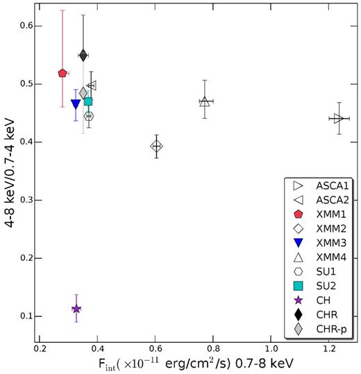
Ratio of the model flux in the 4.0–8.0 keV range to the 0.7–4.0 keV range versus total intrinsic flux, in units of erg s−1 cm−2, from 0.7 to 8.0 keV. Hollow symbols mark observations classified as ultraluminous based on the apparent high-energy curvature of the spectra as described in Section 3.2. The point labelled CH is our new Chandra observation, whereas the point CHR represents the previous Chandra observation by Roberts et al. (2004). A grey diamond labelled CHR-p denotes the hardness ratio of CHR after a 10 per cent pileup correction is applied.
The variation in the hardness ratio over a narrow flux band is significant. Fitting a constant to the observations with fluxes between 3 and 4 × 10⁻¹² erg s−1 cm−2 gives χ2 = 206.61 for six DoF, showing that the hardness ratios are strongly inconsistent with a constant value. We additionally calculate the deviation of the Chandra observation from the weighted average of the other observations and find the difference to be 13.3 times the 90 per cent error. Therefore, the source's spectral evolution clearly does not depend on the luminosity alone.
3.2 High-energy curvature and the ultraluminous state
To investigate the existence of a high energy roll-over in the observations of X-1, we follow the procedure of Gladstone et al. (2009) and fit the spectra with a broken power law (bknpower in xspec) in the 2–10 keV range and compared the goodness of fit to single component models in the same range. Because the single component absorption columns are generally constrained to be below ∼1 × 1022 cm−2 for X-1, the absorption has little effect on data above 2 keV and is poorly constrained in this energy range. We therefore do not include an absorption component in the fits.
Gladstone et al. (2009) suggest that the spectral curvature of the ultraluminous state can only be reliably characterized in high-quality observations with >10 000 counts. Three of the nine observations in our study have fewer than 10 000 counts. The recent Chandra observation is excluded from the table due to its low counts and the low sensitivity of the instrument above 8 keV. We also exclude XMM1 due to its low total counts, though we include XMM4 which has more than 8000 counts. The broken power-law fit parameters are listed in Table 2. For the expected spectral curvature, we require that Γ2 > Γ1 and EBreak be above 2 keV.
Power-law versus broken power law.
| Power law | Broken power law | |||||||
|---|---|---|---|---|---|---|---|---|
| Identifier | Γ | χ2(DoF) | Γ1 | EBreak | Γ2 | χ2(DoF) | Δχ2 | P(F-test) |
| (1) | (2) | (3) | (4) | (5) | (6) | (7) | (8) | (9) |
| ASCA1 | |$1.66^{+0.04}_{-0.04}$| | 203.53(138) | |$1.09^{+0.15}_{-0.17}$| | |$3.4^{+0.3}_{-0.3}$| | |$2.13^{+0.14}_{-0.12}$| | 117.14(136) | 86.39 | 5e-17 |
| ASCA2 | |$1.52^{+0.05}_{-0.05}$| | 117.10(133) | |$1.32^{+0.12}_{-0.14}$| | |$3.9^{+2.3}_{-0.6}$| | |$1.78^{+0.75}_{-0.13}$| | 102.93(131) | 14.17 | 2e-4 |
| XMM2 | |$1.81^{+0.04}_{-0.04}$| | 455.94(379) | |$1.38^{+0.09}_{-0.12}$| | |$3.69^{+0.17}_{-0.21}$| | |$2.26^{+0.10}_{-0.11}$| | 375.49(377) | 80.45 | 1.3e-16 |
| XMM3 | |$1.57^{+0.06}_{-0.06}$| | 222.14(226) | |$1.52^{+0.07}_{-0.03}$| | |$6.6^{+0.8}_{-1.4}$| | |$2.4^{+1.0}_{-0.7}$| | 215.86(224) | 6.28 | 0.04 |
| XMM4 | |$1.67^{+0.05}_{-0.05}$| | 250.59(212) | |$1.29^{+0.13}_{-0.13}$| | |$4.0^{+0.4}_{-0.3}$| | |$2.22^{+0.21}_{-0.17}$| | 205.61(210) | 44.98 | 1.0e-9 |
| Su1 | |$1.68^{+0.04}_{-0.04}$| | 206.61(195) | |$1.54^{+0.07}_{-0.07}$| | |$5.1^{+0.4}_{-0.4}$| | |$2.3^{+0.3}_{-0.2}$| | 180.64(193) | 25.97 | 2e-6 |
| Su2 | |$1.51^{+0.04}_{-0.04}$| | 232.30(207) | |$1.33^{+0.10}_{-0.34}$| | |$3.9^{+0.9}_{-1.1}$| | |$1.70^{+0.12}_{-0.13}$| | 218.93(205) | 13.37 | 0.02 |
(1) Observation identifier; (2) Photon index of PL model; (3) Chi-squared and degrees of freedom for PL fit; (4) Photon index (Bknpower); (5) Break energy (keV); (6) Photon index past break; (7) Chi-squared and degrees of freedom (Bknpower); (8) Chi-square power-law - broken power-law; (9) F-test false rejection probability.
Of the seven observations considered, five are improved with statistical probability of >99 per cent using the F-test. XMM3 is the least improved, with probability 96 per cent. We note that Gladstone et al. (2009) perform similar analysis of the same XMM3 observation and quote an F-test probability of >99 per cent when compared to the power-law model. However, this seems to be a typographical error, and their fit is actually only preferred to 97 per cent based on their tabulated χ2 values.
For comparison we carried out a fit of the spectra of XMM1 and CH despite their low counts, using 0.4–10.0 keV (XMM1) and 0.7–8.0 keV (CH) bands with an absorption factor to utilize as many counts as possible. We find that the photon index breaks to a shallower value in the case of XMM1, disqualifying it based on the criteria above. The broken power-law fit of CH is preferred >99 per cent when compared to a power-law fit. However, CH is better fit by a thermal disc spectrum than a power law (|$\chi ^2_{\rm {disc}}$| = 98.99(108); |$\chi ^2_{\rm pow}$| = 138.70(108)), which causes an exponential cutoff in the spectrum at high energies. Therefore, a broken power law is expected to provide significant improvement over a power law in this case.
We classify into the ultraluminous state those observations where a broken power-law fit is preferred at >99 per cent confidence (excepting the soft, disc CH spectrum) to a simple power law. These observations are represented by hollow symbols in Fig. 1. We note that Rana et al. (2014) have recently confirmed spectral curvature in X-1 up to 30 keV with XMM–Newton and NuStar observations. Using their cutoff power-law fit parameters, we find that this observation would fall in the hard spectral track in Fig. 1 with a hardness ratio of 0.48 and a 0.7–8.0 keV flux of 3× 10⁻¹² erg s−1 cm−2. We observe that the source shows clear spectral curvature in all observations where the flux is above ∼6 × 10⁻¹² erg s−1 cm−2, though we cannot rule out curvature in the lower luminosity observations on the hard track which might occur above the energy range of the instruments used in this study.
3.3 Chandra spectrum
The fit parameters of CH for a simple power law, disc model, and combination are shown in Table 3. The spectrum is best described by a disc model as indicated by bold in the table, though we note that the power-law model cannot be entirely excluded as it is only rejected with 2σ confidence. Although X-1 has generally been observed in a hard, power-law-dominant state, the most recent Chandra observation confirms that X-1 does undergo spectral transitions to an apparently disc-dominant state. The MCD model residuals for CH are shown in Fig. 2.
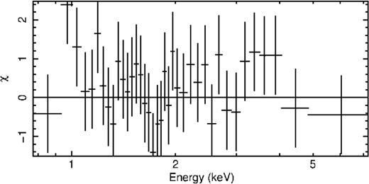
IC 342 X-1 Chandra energy spectrum residuals of the MCD fit.
Chandra spectral fit parameters.
| Model | NH | Γ | Npow | Tin | Ndisc | FX | Int.LX | Disc frac. | χ2(DoF) |
|---|---|---|---|---|---|---|---|---|---|
| (1) | (2) | (3) | (4) | (5) | (6) | (7) | (8) | (9) | (10) |
| Pow | |$1.10^{+0.10}_{-0.09}$| | |$2.98^{+0.15}_{-0.14}$| | |$2.5^{+0.4}_{-0.4}$| | ... | ... | |$2.05^{+0.11}_{-0.11}$| | |$13.6^{+2.2}_{-1.7}$| | ... | 138.70(108) |
| MCD | |$0.56^{+0.06}_{-0.05}$| | ... | ... | |$0.91^{+0.05}_{-0.05}$| | |$0.23^{+0.06}_{-0.05}$| | |$1.93^{+0.09}_{-0.09}$| | |$6^{+4}_{-2}$| | ... | 98.99(108) |
| Pow+MCD | |$0.67^{+0.06}_{-0.05}$| | 2.5# | 0.303# | |$0.87^{+0.06}_{-0.06}$| | |$0.24^{+0.09}_{-0.06}$| | |$1.99^{+0.08}_{-0.08}$| | |$6.4^{+0.6}_{-0.5}$| | >0.71 | 101.61(108) |
(1) Model used for spectral fit; (2) Total absorption column (1022 cm−2); (3) Power-law photon index; (4) Power-law normalization (× 10−3); (5) Inner-disc temperature; (6) Disc normalization; (7) Absorbed flux (0.5–10 keV) (× 10−12 erg s−1 cm−2); (8) Unabsorbed luminosity (0.5–10 keV) for D = 3.9 Mpc (× 1039 erg s−1); (9) Disc fraction: intrinsic disc flux/total flux in 0.5–10 keV range; (10) χ2 and degrees of freedom.
|$\#$|Parameter held fixed during fitting.
The most recent Chandra observation is well fitted by a single-component MCD model. When fitted with a two-component MCD plus power-law model, the power-law component contributes less than 30 per cent of the total flux in the 0.5–10 keV range.
4 RADIO OBSERVATIONS
Radio jets have been observed from stellar mass BHBs, supermassive BHs and, recently, ULXs (Webb et al. 2012; Middleton et al. 2013; Cseh et al. 2014). We carried out radio observations of X-1 using the Jansky Very Large Array (JVLA) of the National Radio Astronomy Observatory (NRAO2) simultaneously with the Chandra X-ray observations on 2012 October 29, from 06:38 to 09:38. The longest baseline, A-array configuration, was used (program SD0164) to test the compactness of previously reported radio emission coincident with the ULX. We observed the source for 55 min at C band (4.5–6.5 GHz) and X band (8.0–10.0 GHz) both with ∼2 GHz bandwidth. The flux and bandpass calibrator referenced was 3C147, and the phase calibrator was J0228+6721. We processed our continuum data using the Common Astronomy Software Application package (casa3) version 4.0 using standard calibration procedures. We also used standard procedures for imaging, and used Briggs weighting with the robust parameter set to 0 to create radio images at both frequencies. The parameters of the resulting images, including the restoration beam size returned by the clean utility and the rms noise level, are listed in Table 4.
Radio image parameters and source detection limits.
| Date | Config. | Freq. | Width | R | 3σ | Beamsize |
|---|---|---|---|---|---|---|
| (1) | (2) | (3) | (4) | (5) | (6) | (7) |
| 10/29/12 | A | 9 | 2 | 0 | 18.9 | 0.21 × 0.14 |
| 10/29/12 | A | 5.5 | 2 | 0 | 19.2 | 0.31 × 0.23 |
| 10/29/12 | A | 5.5 | 2 | 2 | 13.5 | 0.46 × 0.37 |
| 07/03/11 | A | 4.9 | 0.256 | 2 | 26.7 | 0.54 × 0.45 |
| 04/25/08 | C | 4.8 | 0.05 | 0 | 45 | 1.6 × 1.2 |
| 12/06/07 | B |
(1) Observation date; (2) VLA array configuration; (3) Central frequency of bandwidth (GHz); (4) Bandwidth (GHz); (5) Briggs weighting parameter used to make image; (6) Three times the rms value ( μJy beam− 1); (7) Beam size (arcsec)2.
4.1 Search for compact core emission
We estimated the maximum radio flux from X-1 at the position determined by Feng & Kaaret (2009) of R.A. = |$3^{\rm h}45^{\rm m}55{^{\rm s}_{.}}612$|, Dec. = +68°04′55|${^{\prime\prime}_{.}}$|29 (J2000.0) with a 0.21 arcsec error circle at the 90 per cent confidence level. Using a conservative search region with twice the error circle radius, we find no radio emission above the 3σ rms noise level at either frequency. We can therefore place upper limits on the compact core emission from the new JVLA observations at 14 μJy at 5.5 GHz. To bring out emission from the surrounding nebula, we additionally imaged the 5.5 GHz data using robust = 2 (natural) weighting, but still find no significant emission associated with the position of the ULX. Using a restoring beam size in the clean task of the previous VLA observations, 1.6 × 1.1 arcsec2, we are able to bring out some of the features of the surrounding radio nebula but still detect no significant emission in the ULX region (see Fig. 3). This non-detection agrees with observations with the EVN reported by Cseh et al. (2012) and supports their conclusion that the emission reported in the 2007 and 2008 VLA observations was likely a knot of radio emission from the surrounding nebula which is over-resolved in the newest observations because of their larger array configuration.
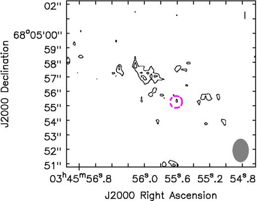
5.5 GHz image from our most recent JVLA observations. The image was produced with natural (Briggs=2) weighting where we have used a restoring beam size of 1.6 × 1.1 arcsec2 in the clean process to match the beam size of the previous VLA observations where possible unresolved emission was reported (Cseh et al. 2012). Contours are drawn at two and three times the rms level of 5.1 μJy beam− 1. The ULX error circle is indicated by a pink circle. No emission above the 3σ level is detected within the ULX region. The restoring beam is drawn as a filled ellipse in the bottom right corner.
To investigate whether the previously reported emission was due to a knot of emission or alternatively a transient event, we reanalysed the previous VLA data consisting of two 3.2 h observations at 4.8 GHz. One observation was made using the VLA's B-array on 2007 December 6 and a second with the C-array on 2008 April 25, 141 d later. We posit that in combining the data from the two arrays, extended emission from the radio nebula observed by the C-array could appear artificially compacted. To test this, we combined the B and C array data and compared the peak emission in the ULX region when the uv range (the range of included baseline lengths) is restricted to be greater than 35kλ, thus excluding extended emission from the shortest baselines, while still including data from the longest baselines of the C-array. If a point source is present, it should be visible to all of the long baselines and the flux of the compact emission should not decrease significantly when the short baselines are omitted. Using Briggs = 0 weighting for both cases (the original combined versus the uv-restricted combined data), we find that the maximum flux in the ULX region decreases from 91 μJy (six times the rms level of 15 μJy beam− 1) to 63 μJy (three times the rms level of 21 μJy beam− 1) when the short baselines are omitted. Thus we do not find a highly significant detection using conditions optimized for compact emission, in agreement with the discussion of Cseh et al. (2012).
4.2 Diffuse emission near X-1
The emission near X-1 could be attributable to a knot from the surrounding radio nebula, or possibly to expanded ejecta from the ULX as was observed in the ULX Holmberg II X-1 by Cseh et al. (2014). To estimate the minimum size of the knot near the ULX, we analysed 4.9 GHz observations that we made with the JVLA in the A-array on 2011 July 3 (project 11A-173). The source was observed for 97 min. The flux and bandpass calibrator referenced was 3C147, and the phase calibrator was J0410+7656. These observations were not coincident with X-ray observations, and were taken in the early testing mode of the new correlator and restricted to a smaller bandwidth of 256 MHz and centred on 4.9 GHz and are subsequently at a slightly lower resolution to our most recent JVLA data with a naturally weighted beam size of 0.54 × 0.45 arcsec2. Again, we find no significant emission in the error circle of the ULX with a peak flux in the ULX region of 1.9 times the rms level of 8.9 μJy beam− 1. Creating an image using a restoring beam size of 1.6 × 1.6 arcsec2 in the clean task, we are able to bring out some of the extended emission to the NE of the ULX, shown in Fig. 4, though the emission in the ULX region is still only 2.4 times the rms level of 13.3 μJy. The 0.5 arcsec beam diameter of the 2011 JVLA image is 1/7 times that of the previous VLA observation with beam size 1.6 × 1.1 arcsec2. In order for the ∼ 63 μJy source to fall below the 3σ rms noise level, it must be spread over at least two beams in the 2011 data, and thus larger than |$\sqrt{2} \times 0.5$| arcsec or ≳13 pc at 3.9 Mpc. This minimum is comparable to size of ejecta observed in Holmberg II X-1 (Cseh et al. 2014). Therefore, from our current data we cannot rule out the possibility of emission due to expanding ejecta from the ULX, though further observations would be necessary to study such an interpretation.
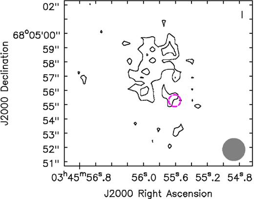
Previous 2011 A-array 5 GHz image with natural (Briggs=2) weighting where we have used a restoring beam of 1.6 × 1.6 arcsec2 to bring out the extended features in the surrounding nebula. Contours are drawn at two and three times the rms level of 13.3 μJy beam− 1. The ULX error circle is indicated by a pink circle. The maximum level of emission within the ULX region is 2.4 times the rms level. The restoring beam is drawn as a filled ellipse in the bottom right corner.
5 DISCUSSION
From the HID in Fig. 1, it is clear that IC 342 X-1 (X-1) is in a different spectral state in the most recent Chandra observations than has been observed previously. However, the flux of X-1 in this state is the same as in harder observations; therefore the spectral state of X-1 cannot be determined by the luminosity alone. This is illustrated in Fig. 5, where the model and spectra are compared for the recent Chandra observation and a previous XMM–Newton observation of the source. These observations are very similar in flux (5 per cent difference using best-fitting single-component models), but have very different spectral shapes. The spectral states of BHBs (Remillard & McClintock 2006) and some ULXs have also been shown to be degenerate with luminosity, and Grisé et al. (2010) showed similarly for the ULX Ho II X-1 that spectral transitions occurred without a significant change in luminosity.
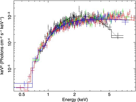
Unfolded model and spectrum of XMM3 (RGB) and CH (black) observations plotted in E2f(E).
Based on high-energy spectral curvature, X-1 appears to be in a super-Eddington state in its highest luminosity observations, as has been suggested by previous authors (Watarai et al. 2001; Ebisawa et al. 2003; Feng & Kaaret 2009; Yoshida et al. 2013). This spectral curvature has been theorized to be the result of heavy Comptonization by a cool, optically thick corona when the source is in a high accretion state (Gladstone et al. 2009). However, at low luminosity X-1 appears to transition to a sub- or near-Eddington accretion state where high-energy curvature is less significant. Sutton et al. (2013) suggested that many ULXs are found in a ‘broadened’ disc state at their lowest luminosities, and transition into ‘hard ultraluminous’ and ‘soft ultraluminous’ states with increasing luminosity, which may represent a transition from near-Eddington to super-Eddington accretion. The new Chandra observation is consistent with the broadened disc classification. However, we note that there is no path to a classical disc state in the Sutton et al. (2013) classification scheme.
The ASCA1 and ASCA2 observations have been interpreted as a transition between a disc-dominated state and a power-law-dominated state (Kubota et al. 2001). The ASCA1 observation, which is well modelled by a disc spectrum, appears on the hard track of the observations in our sample and its hardness is not significantly different from the ASCA2 observation. Sutton et al. (2013) point out that a hard ultraluminous spectrum with some soft excess could be misidentified as a broadened disc spectrum, which could be an explanation for the ASCA1 observation.
At high accretion rates, the disc is expected to be described by an optically thick ‘slim’ disc state, in which cooling by advection becomes a non-negligible factor. As modelled by Watarai et al. (2001), the luminosity–temperature relationship in the slim disc regimes deviates from the standard L ∝ T4 relationship such that, for a super-Eddington system, the mass calculated at a given luminosity and temperature for a thin disc would yield an over-estimate. Because X-1 may be near-Eddington, we additionally fit the Chandra spectrum with a slim disc model developed by Kawaguchi (2003). When fitting with a slim disc model, some authors have found disc-dominated ULX spectra to be better fit by a two-component model that includes Comptonization in addition to a slim disc component rather than the slim disc alone (e.g. Middleton, Sutton & Roberts 2011; Middleton et al. 2012). We find that the Chandra spectrum is well fitted by the Kawaguchi (2003) model number 7 which includes a Comptonized local spectrum and relativistic effects. This model has also been used to fit other ULX spectra (e.g. Foschini et al. 2006; Vierdayanti et al. 2006; Godet et al. 2012; Bachetti et al. 2013). The parameters of the slim disc fit are listed in Table 5. This model assumes a non-rotating BH and that the source is face-on, due to complications of the model for inclined geometries. We find a mass of |$77^{+27}_{-10} \,\mathrm{M_{{\odot }}}$| with the slim disc model, which would increase in the case of a rotating black hole. The best-fitting mass accretion rate is 9.7 in units of LEdd/c2, where |$\dot{M} = L/\eta c^2$|. The Eddington fraction is |$\dot{M}/ M_{\rm Edd} = \eta \dot{M}$|, where the efficiency factor, η, depends on the accretion rate and mass of the BH. Ebisawa et al. (2003) plot the values of η for a slim disc model as a function of mass and |$\dot{M}$| in their fig. 7. For our best-fitting slim disc model parameters, η ∼ 1/16, which yields an accretion rate of ∼60 per cent of the Eddington rate.
Slim disc fit parameters.
| NH | M | |$\dot{M}$| | α | Nslim | χ2(DoF) |
|---|---|---|---|---|---|
| (1) | (2) | (3) | (4) | (5) | (6) |
| |$0.71^{+0.07}_{-0.06}$| | |$77^{+27}_{-9}$| | |$9.7^{+0.8}_{-2.1}$| | |$0.10^{+0.03}_{-0.04}$| | 6.56 × 10⁻⁶# | 99.66(107) |
| NH | M | |$\dot{M}$| | α | Nslim | χ2(DoF) |
|---|---|---|---|---|---|
| (1) | (2) | (3) | (4) | (5) | (6) |
| |$0.71^{+0.07}_{-0.06}$| | |$77^{+27}_{-9}$| | |$9.7^{+0.8}_{-2.1}$| | |$0.10^{+0.03}_{-0.04}$| | 6.56 × 10⁻⁶# | 99.66(107) |
(1) Total absorption column (1022 cm−2); (2) Black hole mass; (3) Mass accretion rate (LEdd/c2); (4) Viscosity; (5) Normalization ((10kpc/d)2); (6) χ2 and degrees of freedom.
|$^\#$|Parameter held fixed during fitting.
In JVLA observations simultaneous with the Chandra observations, no coincident emission is detected above the 3σ noise level of 13.5 μJy, which is consistent with X-1 being in a thermal X-ray state and the derived BH mass. This non-detection is also consistent with 1.6 GHz EVN observations in 2011 June when the source was observed to be in an apparent hard state by Swift (Cseh et al. 2012) and with observations with the JVLA in 2011. We therefore cannot independently confirm the thermal state with the current radio observations, which do not show radio emission being quenched compared to other spectral states (Corbel et al. 2000). Additionally, if X-1 is near the low end of the estimated mass range, the radio emission in the hard state would likely be a few μJy (Merloni et al. 2003), below the sensitivity of current observations.
After reanalysis of 2007 and 2008 VLA observations, we agree with the conclusion of Cseh et al. (2012) that the previously reported emission was likely not due to compact emission from a radio flare, though we cannot entirely rule out a radio flare with the current data. Microquasar flares (Blundell, Schmidtobreick & Trushkin 2011; Corbel et al. 2012; Punsly & Rodriguez 2013) are observed to be approximately 1–10 Jy at a distance of ∼8 pc, which corresponds to 4–40 μJy when scaled for the distance of 3.9 Mpc to IC 342, on the order of the unresolved emission of 63 μJy we find in the 2007–2008 VLA data.
If the emission in the previous VLA observations was due to a radio knot, we can set a lower limit to its linear size based on the resolution of the 2011 JVLA observations. The beam diameter of the naturally weighted 4.9 GHz image is 0.5 arcsec, and in order for the source observed in previous VLA observations to fall below 3σ per resolution element, it must be spread across more than two beams in the higher resolution observations, corresponding to a linear size of ≳13 pc at 3.9 Mpc. This is larger but still comparable to size of ejecta observed near the ULX Holmberg II X-1 by Cseh et al. (2014), and one possible interpretation is that the observed knot of emission is expanded ejecta from the ULX. However, the radio field surrounding X-1 is complex and higher signal-to-noise ratio observations would be necessary to make any strong conclusions.
ACKNOWLEDGMENTS
Support for this work was provided by the National Aeronautics and Space Administration through Chandra Award Number GO2–13036X issued by the Chandra X-ray Observatory Center, which is operated by the Smithsonian Astrophysical Observatory for and on behalf of the National Aeronautics Space Administration under contract NAS8–03060. SC acknowledges funding support from the French Research National Agency: CHAOS project ANR-12-BS05-00094 and financial support from the UnivEarthS Labex program of Sorbonne Paris Cité (ANR-10-LABX-0023 and ANR-11-IDEX-0005-02). We thank the anonymous referee for her/his comments and suggestions which contributed to the improvement of the paper.
The National Radio Astronomy Observatory is a facility of the National Science Foundation operated under cooperative agreement by Associated Universities, Inc.
