


Abstract
The timing errors for individual planetary transits using the photometric transit timing technique (TTVp) are derived for light curves contaminated with either white additive noise, realistic stellar noise or filtered stellar noise. For the case of white noise, the timing errors are derived analytically, while timing errors for realistic and filtered noise are numerically derived using solar data from the Solar and Heliospheric Observatory satellite. These results are then used to explore the conjecture that moons of transiting planets become easier to detect using the TTVp method the farther their planet is from the star. Using transit duration as a proxy for planet–star distance, it is found that in the case of realistic stellar noise, an increase in star–planet distance/transit duration does not necessarily lead to an increase in moon detectability.
1 INTRODUCTION
The possibility of detecting planets around other stars by measuring the dip in the host star's intensity as the planet transits across its disc was first suggested by Struve (1952). With the advent of wide field CCD surveys and the launch of the CoRoT and Kepler satellites, this planet detection method has come of age with over 280 transiting planets known.1 Not only does the transit technique allow for planetary detection, it also allows for the measurement of observables which allow tests of theories of planet formation and structure. For example, measurements of the orbital orientation relative to the star's spin axis (e.g. Queloz et al. 2000; Narita et al. 2007; Triaud et al. 2010) facilitate tests of theories of planetary migration (e.g. Fabrycky & Tremaine 2007), and detection or non-detection of moons, using e.g. the methods proposed by Sartoretti & Schneider (1999), can be compared with mass limits predicted from planet formation models (e.g. Wada, Kokubo & Makino 2006; Sasaki, Stewart & Ida 2010).
In order for this scientifically valuable data to be obtained, the planetary nature of transiting planet candidates must be confirmed. For bright, slowly rotating stars this could involve measurement of planetary mass through detection of the radial velocity signal (e.g. Marcy & Butler 1992), while for dimmer stars this could involve using transit timing variations in multiplanet systems (e.g. Holman & Murray 2005) or additional photometric effects such as beaming, elipsoidal and rotation effects (Faigler & Mazeh 2011). In addition, as systems capable of mimicking all the photometric and timing effects corresponding to a physically realistic moon system are likely to be rare, and as moon formation is predicted to be a common outcome of planet formation (e.g. Elser et al. 2011), another possible avenue for planetary followup would be the detection of a moon or a system of moons of a given candidate planet.
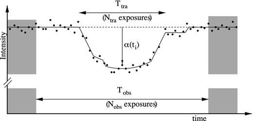
An example transit showing measured intensities (dots) and theoretical intensity (line). The quantity α(ti) is shown for one of the exposures and the region which is outside the window that is counted in the sum is shaded grey.
The detectability of moons using the TTVp technique is determined by the size of the timing perturbations they produce relative to the error in the measured value of τ due to photometric noise. In the investigation of Szabó et al. (2006) into moon detectability using this technique, a number of simplifying assumptions were made, including assuming that the noise in the light curve was white, that is, the noise is Gaussian and uncorrelated. Unfortunately not all photometric noise sources relevant to transit surveys are white.
Intrinsic photometric variability of most Sun-like stars is known to be a red noise process (e.g. Lockwood et al. 2007), that is, the noise is characterized by a sloping spectral energy distribution with extra power in the low frequencies or the ‘red’ end of the spectrum. Due to this excess of long wavelength components, consecutive data points in a light curve dominated by the intrinsic variability of the host star are correlated. It has long been known that red photometric noise due to stellar variability is a limiting factor in transit surveys (e.g. Borucki, Scargle & Hudson 1985). Consequently, it is of interest to determine the effect of this type of noise on the error in τ, and thus moon detectability. Also, as an increasing number of algorithms developed for transit detection use a pre-whitening filter, it is also of interest to determine the effect of filtering on the error in τ.
Finally, in addition to being a method proposed to search for moons and follow up planets, Oshagh et al. (2012) have used this method to try and detect additional planet-mass bodies in the LHS 6343 system by looking for dynamically induced timing perturbations in the transits of the brown dwarf LHS 6343 C across the M star LHS 6343 A. The methods presented here could also be applied to this system.
With these aims in mind, in Section 2 a framework for calculating the noise in τ due to photometric variability is developed. In Sections 3, 4 and 5, this framework is then used to determine the noise in τ as a function of observing duration and exposure time for the cases of white noise, realistic stellar noise and filtered stellar noise, respectively. In Section 6, the results from Sections 3, 4 and 5 are used to investigate the relationship between moon detectability and increasing transit duration for this technique.
2 THEORETICAL GROUNDWORK
Equations (11), (14) and (15) provide a simple method for determining a sequence of ϵj values for a transit with a given Ap + Am, using out-of-transit light curves. This formulation will be used to analyse the cases of realistic and filtered stellar noise.
3 WHITE NOISE: ANALYTIC DERIVATION
3.1 Introduction to white noise
White noise is a type of additive noise which occurs in many physical processes such as photon counting. It is known as white, as the Fourier transform of white noise contains the same power at all frequencies.
3.2 Derivation of ϵj
This expression can be simplified by considering the relative sizes of the terms. Recalling from Section 2 that both Δτ and Δtp are much smaller than ti − (jTp + t0), and following the procedure used to simplify equation (9), we can also neglect the Δtp term from equation (23).
To check this formula, a Monte Carlo simulation was run. A mock transit light curve was constructed using three straight line segments corresponding to the ingress, flat bottom and egress. To this, Gaussian noise with a known standard deviation was added to produce a sequence of model transit light curves. For each light curve, the ϵj value, that is, the difference between the centre of the transit and the value of τ, was calculated. The histogram of the errors of these model light curves and the theoretical prediction are both shown in Fig. 2. As can be seen the agreement is very strong.
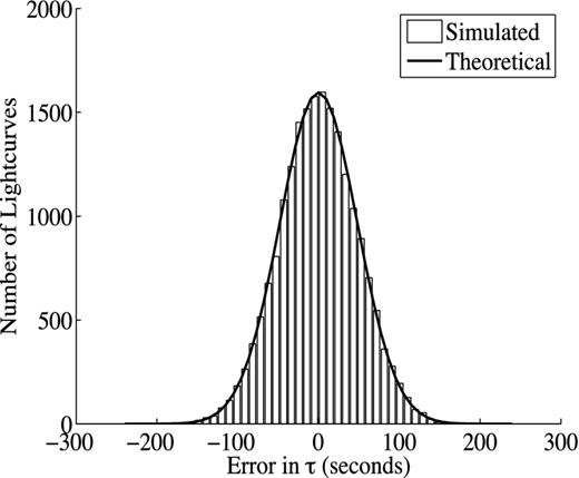
Comparison between a Monte Carlo simulation (white bar) and theoretical prediction (black line) for the distribution of ϵj values for a noisy transit.
3.3 Relationship between moon detectability and exposure time
Szabó et al. (2006) found that a decrease in exposure time leads to an increase in moon detectability. From equation (2), we see that there are two candidate causes for a relationship between exposure time and moon detectability using the TTVp. First, that the calculated value of τ may depend on the timing and duration of the exposures, and second, that the exposure time alters the characteristic size of σϵ, thus modifying moon detectability. It turns out that for transit parameters corresponding to the planetary systems of interest, the timing and duration of exposures does not significantly alter the calculated value of τ (see Appendix A). Consequently, we can investigate the relationship between moon detectability and exposure time by investigating the relationship between σϵ and exposure time using equation (29).
To begin, consider the first term in square brackets in equation (29). This term describes both the dependence of σϵ on the relative photometric accuracy (σL/L0) and the exposure time (Δt). Unsurprisingly, the smaller the relative photometric error, the smaller the value of σϵ and consequently, the smaller the error in τ. However, while the relative photometric noise can be altered without changing the exposure time, for example, by moving to a larger telescope or by upgrading the instrumentation, changing the exposure time can alter the photometric noise depending on its source. For the case of shot noise, error due to small number statistics, the total error is proportional to the square root of the total number of photons collected for that star (i.e. |$\sigma _L \propto \sqrt{\Delta t}$|) while the total intensity is proportional to the total number of photons (i.e. L0 ∝ Δt), so the relative photometric error is proportional to |$\sqrt{\Delta t}/\Delta t = (\Delta t)^{-1/2}$|.3 For the case of read noise, error resulting from the process of measuring the number of photons collected at the end of an exposure, the total error does not depend on the exposure time. Consequently, the relative photometric error is proportional to (Δt)−1. So, for a star with white photometric noise that is dominated by shot noise, σϵ is independent of exposure time, while for a star dominated by read noise, σϵ should decrease with increasing exposure time.4
4 RED NOISE: OBSERVATIONAL DERIVATION
4.1 Introduction to red noise
Red noise is additive noise which contains a surplus of power at the lower (or ‘redder’) frequencies. While in signal processing, red noise refers to Brownian noise or random walk noise and has spectral density proportional to f−2, where f is the frequency, in astrophysics, the term is colloquially used to describe any noise process which produces an excess of low frequencies.
The fact that stars in general (e.g. Dorren & Guinan 1982; Radick et al. 1982) and the Sun in particular (e.g. Willson et al. 1981) have a red noise component in their light curves has long been known. Due to this excess of long wavelength components, consecutive data points in a light curve dominated by the intrinsic variability of the host star are correlated, that is, there are long-term trends in the data (see Fig. 3). Consequently, the statistical methods used in the previous section no longer apply. As mentioned in Section 2, for the case of realistic photometric noise, the distribution and behaviour of ϵj are calculated numerically, in particular, using solar photometric light curves.
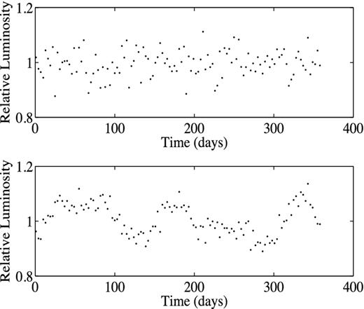
Comparison between white noise (top panel) and red noise (bottom panel).
4.2 Discussion of suitability of solar photometric data for calculating ϵj
In order to determine the effect of intrinsic stellar photometric variability on ϵj using equation (14), a suitable sample light curve which is dominated by realistic photometric stellar variability corresponding to a typical star is required. This data series should optimally have a number of properties. First, it needs to be long enough such that a statistically valid estimate of ϵj can be constructed. Secondly, the data must have high signal-to-noise ratio to ensure that the majority of recorded photometric noise is inherent to the star, and not resulting from instrumental or statistical effects. Thirdly, the data need to be high cadence, such that the effect of long and short exposure times on ϵj can be investigated. Finally, this data must be easily available and easy to manipulate. Fortunately, photometric measurements of the Sun meet all these requirements.
Over 12 yr of high-quality solar data are available as a result of the Solar and Heliospheric Observatory (SoHO). This satellite is positioned at the L1 point between the Earth and the Sun, which allows it uninterrupted access to the Sun's behaviour. For this work, it is the measurements of Total Solar Irradience, the total intensity of the solar face, that are important. This measurement is made within the VIRGO (Variability of solar IRradiance and Gravity Oscillations) module (Fröhlich et al. 1995), by comparing the output of the photometers PMO6V (PMO6-type radiometer on VIRGO, indicated by a V) and DIARAD (DIfferential Absolute RADiometer) (Fröhlich et al. 1997). These data were kindly made available by the SoHO team and can be freely downloaded from the SoHO archive.5
While high-quality solar data may be freely available, whether it should be used depends on whether the photometric behaviour of the Sun is representative of the photometric behaviour of Sun-like stars, in particular, the stars to be targeted by CoRoT and Kepler. Indeed, it has been found that the Sun shows two to three times less variation on the decadal time-scale compared to similar stars (Lockwood, Skiff & Radick 1997; Radick et al. 1998; Lockwood et al. 2007). In addition, these findings are in agreement with the preliminary findings from the CoRoT (e.g. Aigrain et al. 2009) and Kepler (e.g. Basri et al. 2010; McQuillan, Aigrain & Roberts 2012) satellites. While this discrepancy may seem discouraging, it needs to be viewed in the context of two other findings: the effect of star orientation with respect to the observer, and the results of studies of extra-solar planet host stars. First, it has been suggested that the low observed value of solar photometric noise is due to our privileged observing position, that is, in the plane of the Sun's equator. The maximum predicted magnitude of this effect ranges from an increase in photometric variability of 6 (Schatten 1993) to 1.3 (Knaack et al. 2001) times that observed in the equatorial plane as the viewing angle is altered. Fortunately, it has been observed for both non-transiting (Le Bouquin et al. 2009) and transiting planets that there is a preference for the orbital angular momentum vector of the planet and the spin axis of the host star to be aligned. For the case of transiting planets there is a population of hot Jupiters with orbits that are not aligned with the stellar equator (e.g. Triaud et al. 2010); however, Triaud (2011) finds that the degree of orbital misalignment is related to the age of the star, and in particular is reduced for older systems, possibly as a result of tidal interactions between the planet and the star. Consequently, as the planets of interest transit, the equator of the target star is likely to be preferentially aligned with the line of sight. Secondly, while the survey conducted by Lockwood et al. (2007) into the photometric variability of Sun-like stars is the most temporally complete, it is not the only survey. In particular, the survey of Henry et al. (2000) has looked at the photometric variability of extra-solar planet host stars detected by the radial velocity technique. Within this subset, the Sun appears typical. Unfortunately, as only relatively magnetically inactive stars are chosen as targets for radial velocity searches, and long-term photometric variability increases with increasing magnetic activity (e.g Radick et al. 1998), this set of stars is statistically biased. Consequently, the study of Henry et al. (2000) cannot be used to argue that the Sun's photometric stability is representative of most stars. However, while not all planetary hosts will display the same photometric stability as the Sun e.g. CoRoT-2b (Alonso et al. 2008), this study does indicate that there is a substantial subset of planetary host stars which will. As this is a first investigation into the effect of realistic stellar photometric noise on the TTVp technique, and solar photometric noise is relatively representative of stellar photometric noise, solar data were used as a test bed for this analysis. However, we note that the procedure described here could be applied to the photometry of other stars.
4.3 Derivation of ϵj
As, in this case, the distribution of ϵ⊙ will be numerically determined, a finite number of values of the independent variables, in this case the exposure time Δt and the observing duration Tobs, need to be selected. It was decided to use observing durations of 0.5, 1, 2, 4, 8, 12, 24 and 36 h to cover the most extreme systems likely to be encountered. For comparison, GJ 436 b, a planet with a relatively short transit duration, takes just over 1 h to transit its host, while the Earth would take up to 13 h to transit the central chord of the Sun. In addition, it was also decided to investigate exposure times representative of those used by the satellites CoRoT and Kepler. For the case of CoRoT, a 16 min exposure time is used for its catalogue of approximately 12 000 targets, but it is also capable of a 32 s readout for a subset of 1000 highlighted sources (Quentin et al. 2006). For the case of Kepler, a 30 min exposure time is used for its set of approximately 150 000 sources, but it is also capable of 1 min exposures for a subset of 512 highlighted sources (Borucki et al. 2008). So, ideally, it would be useful to compare the distribution of ϵj for the case of ‘short’ exposures (32 s or 1 min) and ‘long’ exposures (16 or 30 min).
As the two photometers on the VIRGO module, PMO6V and DIARAD have exposure times of 1 and 3 min, respectively, it was decided to use these individual exposures as the ‘short’ exposures, and artificially construct the long exposures, by dividing the data into 30 min segments and then co-adding all exposures within each segment. To investigate the suitability of the data from the two photometers for this analysis, the number of valid data segments for each pair of possible exposure time and observing duration was determined for each photometer (see Table 1). As a result of the dearth of contiguous sequences of data within the PMO6V data set, it was decided to use the DIARAD data, and consequently to use 3 min as the ‘short’ exposure time.
Number of complete lengths of data of a given duration, Tobs, for each of the four possible data sets.
| DIARAD | DIARAD | PMOV6V | PMOV6V | |
|---|---|---|---|---|
| Tobs | 3 min | 30 min | 1 min | 30 min |
| 30 min | 163 039 | – | 132 185 | – |
| 1 h | 78 971 | 76 956 | 63 802 | 61 681 |
| 2 h | 37 208 | 36 244 | 29 736 | 29 604 |
| 4 h | 16 503 | 16 113 | 12 657 | 12 153 |
| 8 h | 6471 | 6318 | 4077 | 3679 |
| 12 h | 3438 | 3365 | 475 | 462 |
| 16 h | 2080 | 2038 | 238 | 228 |
| 24 h | 824 | 805 | 73 | 71 |
| 36 h | 317 | 307 | 54 | 53 |
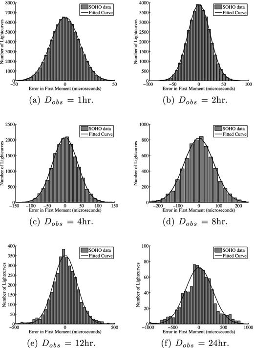
The distribution of ϵ⊙ was calculated for each pair of exposure time and observation duration as follows. The raw level 1.8 irradience data from SoHO were converted to level 2 data using the tables given on the SoHO website.6 These data then needed to be analysed. For the case of 3 min exposures, this involved dividing the sequence into sequences of valid data of length Tobs. For the case of 30 min exposures, the data were first pre-processed by dividing it into sets of 10 contiguous exposures and treating each of these lengths as a single exposure. This was done by co-adding the exposures for the case where all the exposures were valid, or by recording an invalid intensity for the case where they were not. These pre-processed data were then divided into lengths of valid data of length Tobs. ϵ⊙, the difference between the central time and first moment of each of these lengths, was then calculated using equations (11) and (15), and the values binned to produce a frequency histogram (see Fig. 4). As all the distributions were approximately normal and had zero mean, they could be fully described by their standard deviation. The values of σ⊙, the standard deviation of ϵ⊙, along with their associated observing duration and exposure time are presented in Table 2.
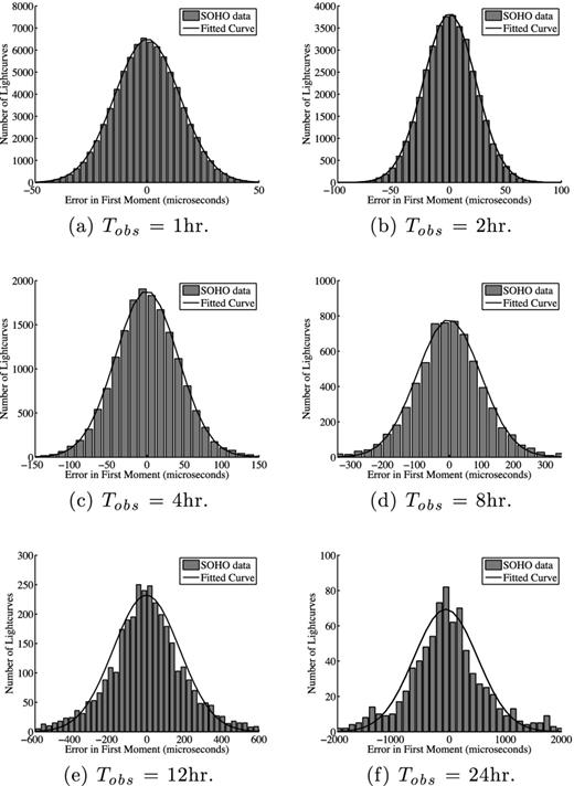
The observationally determined distribution of ϵ⊙ (grey bar) for the case of realistic solar photometric noise for six different length observing windows. For observing windows less than 12 h long, the distribution of ϵ⊙ is very nearly a normal distribution (black line). Note the different scales.
The size of σ⊙ for the case of realistic stellar noise, as a function of length of observation window, Tobs, and exposure time Δt. The value in parentheses is the error in the last significant figure.
| Tobs | Δt = 3 min | Δt = 30 min |
|---|---|---|
| 30 min | 9.49(1) × 10−3 s | – |
| 1 h | 1.4507(2) × 10−2 s | 1.248(1) × 10−2 s |
| 2 h | 2.3201(7) × 10−2 s | 2.232(1) × 10−2 s |
| 4 h | 4.178(4) × 10−2 s | 4.160(4) × 10−2 s |
| 8 h | 9.863(3) × 10−2 s | 9.77(2) × 10−2 s |
| 12 h | 1.78(1) × 10−1 s | 1.760(4) × 10−1 s |
| 16 h | 2.85(1) × 10−1 s | 2.86(1) × 10−1 s |
| 24 h | 5.6(1) × 10−1 s | 5.7(1) × 10−1 s |
| 36 h | 1.15(4) s | 1.14(3) s |
As can be seen in Table 2, the values of σ⊙ for both exposure times, for Tobs greater than 4 h agree to within a few per cent. As the vast majority of realistic values of Tobs are likely to be greater than 4 h, these two data sets are effectively equal. As can be seen from Fig. 5, the values of ϵj calculated for the cases of realistic solar noise and white noise of the same power7 are in close agreement with those calculated for the case of noise for short transit durations, but diverge for longer transit durations. This divergence is the result of the longer transit durations ‘letting in’ more of the lower frequency components of the noise. Disturbingly, in the investigation by Szabó et al. (2006), they found that the most easily detectable moons are around planets far from their host, with correspondingly long transit durations.
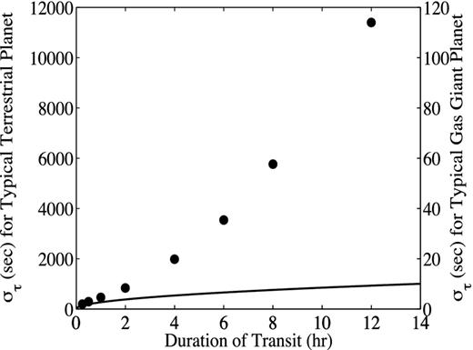
Comparison between measured errors, ϵj using solar light curves (dots) and theoretically predicted ϵj using white noise with the same power as the noise in the solar light curves (thick line). As the results for 3 and 30 min exposures are so similar, only the data for three minute exposures are shown. These relations are shown for the case of the transit of a gas giant (Ap/L0Ntra = 10− 2) and a terrestrial planet (Ap/L0Ntra = 10− 4), assuming Tobs ≈ 2Ttra.
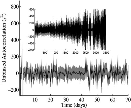
In addition to determining the distribution of ϵj, it is also important to determine whether or not consecutive values of ϵj are correlated. Consequently, the auto-correlation8 of the sequence of ϵj values was computed (see Fig. 6). Physically, we would expect that there would be some correlation on time-scales comparable with the rotational period of the Sun (≈25 d) as the gradient of the luminosity is also correlated over those time-scales. As can be seen from Fig. 6, ϵj is effectively uncorrelated for all transiting planets with orbital periods above 40 d. Assuming a host planet with a Jupiter-like Q-value of 105, we have from Barnes & O'Brien (2002) that the shortest interval between transits, given that the planet has a Ganymede-sized moon is approximately one month. For the case where the Q-value is much higher, 1012–1013, for example, as a result of dependence of the Q-value on the orbital period of the moon, the minimum planetary orbital period, i.e. the minimum time between transits, for giant planets with large dynamically stable moons reduces to a couple of days (Cassidy et al. 2009). Consequently, for the case where the host planet has a Q-value of 105, ϵj is uncorrelated and for the case where the Q-value is higher and the planet orbital period shorter, ϵj may be correlated.
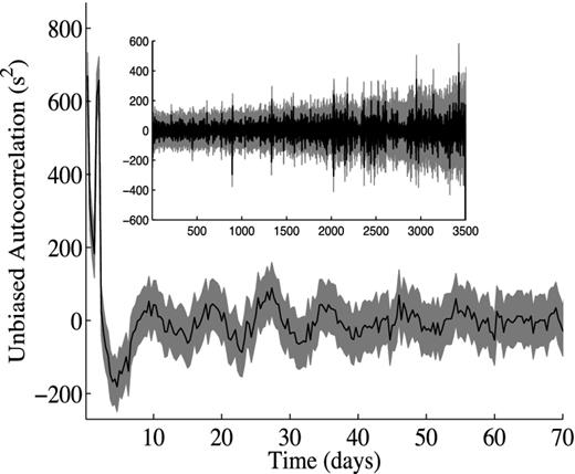
Normalized autocorrelation function of ϵj (black line) calculated using realistic stellar noise for the case where the observing window is 8 h. For reference, the one sigma error bars (grey) are also shown. As short period planets are more likely to be discovered by the transit technique than longer period planets as a result of the higher transit probabilities of short period planets, the inner section of the autocorrelation function is shown in the main plot. For completeness, the full autocorrelation function is shown in the inset.
Now that the case of raw realistic stellar noise has been investigated, the analysis can be refined by ‘filtering’ the data to remove long-term trends. In the case to be investigated these trends are due to the advection of active regions across the solar surface.
5 FILTERED NOISE: OBSERVATIONAL DERIVATION
5.1 Introduction to filtered noise
As the presence of red noise in light curves significantly alters the detection probability of transiting planets (e.g. Borucki et al. 1985; Pont, Zucker & Queloz 2006), a range of methods for reducing the effect of this type of noise have been investigated. These include methods where the physical processes believed to be underlying the red noise are modelled (Lanza et al. 2003), methods where the red noise is pre-processed with a whitening filter before transit detection (e.g. Carpano, Aigrain & Favata 2003; Guis & Barge 2005; Moutou et al. 2005, team 3) and methods where the filtering is performed in combination with a transit finding algorithm (e.g. Jenkins 2002).
As, for this investigation, moon searches will be conducted on a star by star basis, it was decided to use a method which modelled the physical processes appropriate to each star. Consequently, the method selected was the three-spot model method of Lanza et al. (2003) as, it was developed using SoHO data, it was designed to be adapted to model photometric variation for any Sun-like star (Lanza, Rodonò & Pagano 2004), and it has been used to model variability in real stellar data, specifically, the CoRoT targets CoRoT-2 (Lanza et al. 2009b) and CoRoT-4 (Lanza et al. 2009a).9 To provide a reality check, the results for this filtering technique were compared with those calculated using the a simple high-pass filter, such as the one investigated by Carpano et al. (2003).
5.2 Description of the three-spot model
One source of long-term photometric variability of the Sun is rotational modulation of the active regions, that is, regions on the Sun's surface where the magnetic field strengths are high. Active regions are complex structures comprising of clusters of magnetic phenomenon such as darker sunspots and brighter faculae. While there is a lognormal distribution of active region sizes (Bogdan et al. 1988), Lanza et al. (2003) determined that the long-term photometric variation of the Sun could be effectively modelled by only accounting for three distinct active regions on the face of the Sun in any given 14 d window.
To perform the fitting required to implement this ‘three-spot model’, the extent to which the substructure of the active regions needs to be modelled must be determined. In particular, the issues of active region composition, evolution and distribution across the solar surface need to be explored. While the ratio between the area of faculae and sunspots changes as a function of active region size and position in the solar cycle (Chapman, Cookson & Dobias 1997), Lanza et al. (2003) assumed a constant ratio of sunspot area to facular area of 1:10. Consequently, this assumption was also used for this work. Not only are active regions composed of complex structures, these structures evolve over time. Fortunately, the time-scale for active region evolution is longer than that for solar rotation. Consequently, the solar intensity data can be divided into blocks, such that it can be assumed that the position and size of an active region does not change within the block. Lanza et al. (2003) found that a good compromise between modelling the effect of solar rotation and minimizing active region evolution was 14 d.10 Consequently, for this work, data were divided into 14 d segments, each consisting of 6720 data points. In addition, as active regions are generally much smaller than the radius of the Sun, the entire active region can be modelled as having the same μ value, where the μ value is given by the cosine of the angle between the surface normal and the direction of the line of sight at that position on the solar surface. Consequently, three variables are required to model each active region, two describing the position of the region on the face of the Sun, and one variable describing the effective area of the active region. With these assumptions and simplifications in mind, the fitting model can be introduced.
In addition to fitting these 11 variables, there are a number of constraints imposed by the physics of the problem on the values the variables can take, in particular, with respect to sunspot areas and the rotation rate. The values of the sunspot areas were constrained to be positive and below a threshold size. Lanza et al. (2003) calculated this threshold size to be 8.2 × 10⁻⁴ by assuming that the largest dip in the data were due to the rotational modulation of a single active region. However, as the span of SoHO data used for this work is longer than that used by Lanza et al. (2003), the upper limit derived may not be able to explain all the behaviour in the light curve analysed. In particular, there is a region of apparently high sunspot activity occurring between 2003 October 15 and November 11 containing dips which correspond to spots with a relative area of 1.7 × 10⁻³. Consequently, the upper limit of 8.2 × 10⁻⁴ on sunspot area was used for all 14 d blocks except for the two blocks between the 2003 October 15 and the November 11, where the limit 1.7 × 10⁻³ was used. In addition to sunspot area, solar rotation rate is an observationally constrained quantity. For this work, the limits of 23–33.5 d on the solar rotation period, derived by Lanza et al. (2003), were used without modification.
For this work, the simplex method described by Lagarias et al. (1998), implemented using the multidimensional matlab fitting function fminsearch was used to complete this constrained minimization. This approach required that starting values and a function for calculating χ2 were provided to the method. The starting values for each fit were either taken from the previous fit or manually estimated. As suggested by Lanza et al. (2003), the variables, A1, λ1, θ1, A2, λ2, θ2, A3, λ3, θ3 and Lr, were fitted independently to Ω, which was then optimized. In addition, to ensure that the sunspot areas remained within the physical bounds, the function which returned the χ2 value was modified such that it returned a large value if active region areas became too large or negative. Unfortunately, while these inputs resulted in a set of acceptable values for the fitting parameters being returned, issues with the simplex method itself, such as the fact that it may not converge (e.g. McKinnon 1999), required that a number of tests were conducted to ensure that the true minimum had been found.
To ensure that the fit had converged, three checks were made. First, each fit was checked by eye. Secondly, for each block of data, the fitting procedure was repeated, that is, the output of the preceding fit was used as the starting variables for the next fit, until the fitted variables remained approximately the same between two successive fits. Thirdly, the dependence of χ2 on each of the 11 fitting parameters was checked for 29 randomly selected blocks. All curves inspected indicated that for these blocks the simplex method had converged to the χ2 minimum.
Once the fitting had been performed, the best-fitting parameters were recorded. These parameters were in turn used to produce a model light curve. By subtracting the model from the data and then adding the average intensity, a detrended light curve was constructed.
5.3 Derivation of ϵj
This set of detrended data was then subjected to the same procedure as that of the unfiltered red noise (see Section 4.3) to determine σϵ as a function of transit area, transit duration and exposure time. The results are presented in Table 3 and Figs 7 and 8. To provide a reality check, these results were compared to results obtained using a different filtering method. For simplicity, the high-pass filter described in Carpano et al. (2003) was selected. The calculated values of σϵ produced by both methods agree to within 5 per cent.
The observationally determined distribution of ϵ⊙ (grey bar) for the case of solar photometric noise filtered using the method of Lanza et al. (2003), for six different length observing windows. Note that the distribution of ϵ⊙ is very nearly a normal distribution (black line). Note the different scales.
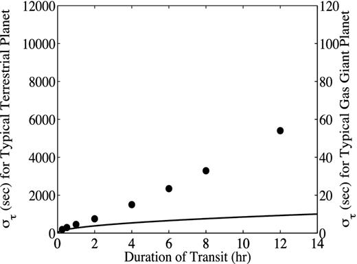
Comparison between measured errors, ϵj using solar light curves which have been ‘filtered’ using the method of Lanza et al. (2003) (dots) and theoretically predicted ϵj using white noise with the same power as the noise in the solar light curves (thick line). These relations are shown for the case of the transit of a gas giant (Ap/L0Ntra = 10− 2) and a terrestrial planet (Ap/L0Ntra = 10− 4), assuming Tobs ≈ 2Ttra.
The size of σ⊙ for the case of realistic stellar noise which has been filtered using the method of Lanza et al. (2003), as a function of length of observation window, Tobs, and exposure time, Δt. The value in parentheses is the error in the last significant figure.
| Tobs | Δt = 3 min | Δt = 30 min |
|---|---|---|
| 30 min | 9.440(5) × 10−3 s | – |
| 1 h | 1.4433(2) × 10−2 s | 1.244(1) × 10−2 s |
| 2 h | 2.264(1) × 10−2 s | 2.181(2) × 10−2 s |
| 4 h | 3.77(1) × 10−2 s | 3.77(1) × 10−2 s |
| 8 h | 7.48(1) × 10−2 s | 7.417(7) × 10−2 s |
| 12 h | 1.169(2) × 10−1 s | 1.157(3) × 10−1 s |
| 16 h | 1.640(8) × 10−1 s | 1.639(6) × 10−1 s |
| 24 h | 2.71(2) × 10−1 s | 2.72(2) × 10−1 s |
| 36 h | 4.3(2) × 10−1 s | 4.2(2) × 10−1 s |
This agreement suggests that the behaviour of ϵ⊙ is not a strong function of the filtering method selected.
Normalized autocorrelation function of ϵj (black line) calculated using filtered stellar noise for the case where the observing window is 8 h. For reference, the one sigma error bars (grey) are also shown. As short period planets are more likely to be discovered by the transit technique, the inner section of the autocorrelation function is shown in the main plot. For completeness, the full autocorrelation function is shown in the inset.
6 SIGNAL TO NOISE AS A FUNCTION OF TRANSIT DURATION
Szabó et al. (2006) found that when the noise on the light curve was white, the further a transiting planet was from its host star, the more detectable are its moons by the TTVp method. As discussed previously, not all noise sources relevant to transit surveys are white. Consequently, it would be useful to investigate whether this result holds for realistic or filtered stellar noise.
The detectability of moons is defined by the size of the timing perturbation they produce relative to the timing noise. So, to determine how the detectability of a moon changes with the transit duration Ttra, the relationship between the size of the timing signal due to a moon and Ttra must be determined and compared with the relationship between the timing noise and Ttra.
For the case of white noise it can be seen from equations (41) and (39) that as the amplitude of the timing signal increases as Ttra and the standard deviation of the timing noise increases as |$\sqrt{T_{\rm tra}}$|, moons become more detectable as Ttra increases. This is in direct agreement with the work of Szabó et al. (2006). For the case where the noise is realistic stellar noise, from equation (44) we have that for short transit durations the standard deviation of the noise increases as Ttra, while for longer transit durations it increases as T2tra. Recalling from equation (39) that the amplitude of the timing signal increases as Ttra, we have that for short transit durations moon detectability is relatively independent of transit duration while for longer transit durations it decreases with increasing transit duration. Finally, for the case of filtered realistic noise, from equations (45) and (39) we have that both the timing signal and noise are proportional to Ttra, so for this case, moon detectability is independent of transit duration.
7 LIMITATIONS OF THIS ANALYSIS
The main assumption in this analysis is that the variability of a light curve during transit is the same as that out of transit. As light from a star is not uniformly distributed across its surface, this assumption will not always be valid. Indeed, finite structures such as starspots were predicted to (Hui & Seager 2002; Silva 2003) and do (e.g. Pont et al. 2007; Sanchis-Ojeda & Winn 2011) alter transit light curves. However, as discrete structures on the stellar surface should act to increase the variability of the light curve during transit, including effects due to these structures will act to make moons even less detectable than in the cases explored in this paper.
8 CONCLUSIONS
The effect of three different types of photometric noise, white, solar and filtered solar, on the TTVp moon detection technique are investigated. In particular, it is found that
the TTVp timing noise is approximately normally distributed and uncorrelated for most physically realistic planet–moon systems.
for the case of white photometric noise, where the noise budget is dominated by photon noise, as well as the cases of solar and filtered solar photometric noise, the timing error is approximately independent of the exposure time.
the timing noise for the case of solar photometric noise is dramatically larger than that for the equivalent amplitude white noise, and while filtering the light curve reduces this effect, it does not remove it.
assuming that the number of observed transits is held constant, for the case where the light curve is dominated by white, solar and filtered solar photometric noise, moon detectability using the TTVp technique increases with increasing transit duration, decreases with increasing transit duration and is independent of transit duration, respectively.
As a result of these findings, non-white photometric variability of host stars needs to be taken into account when analysing TTVp data or deriving moon detection thresholds. In addition, as this work focuses on the TTVp technique, research into the effect of non-white photometric noise on moon detection using other techniques is strongly recommended.
I thank Dr. Daniel Bayliss for informing me of the effect stellar red noise has on planetary transit detectability. In addition, I would like to thank Dr. Rosemary Mardling and Dr. Aidan Sudbury for their invaluable discussions and help improving the transparency of the derivations. Finally, my research was funded through the Faculty of Science Dean's Postgraduate Research Scholarship Scheme at Monash University. This financial assistance is gratefully acknowledged.
See, for example, http://exoplanet.eu/catalogue.php.
Kepler was designed to achieve a relative photometric precision of 2 × 10⁻⁵ over a 6.5 h exposure for the case of the 12th magnitude Sun-like host star (e.g. Basri, Borucki & Koch 2005). For the case of white noise, this translates to a relative photometric precision of 3.95 × 10⁻⁴ for a 1 min exposure.
A similar argument can be constructed for the case of dark noise, the noise caused by electron motion in the CCD chip during an exposure.
For the case where the relative photometric noise is independent of exposure time, such as the case explored by Szabó et al. (2006), σϵ will decrease with decreasing exposure time, which is in agreement with their findings.
Derived in Appendix B.
For this work the autocorrelation is defined as ∑jϵjϵj + k/Nk, where ϵj and ϵj + k represent all ϵj pairs separated by k × 8 h and Nk is the number of such pairs. This unbiased definition was selected to allow ease of comparison between values calculated for different lag times.
The optimum block length depends on the characteristics of the host star. For example, for the case of the Sun the optimal length is 14 d, while for the case of CoRoT-4 a length of 8.2 d (Lanza et al. 2009a) was used.
As there are twice as many terms in the sum in the numerator of the third term in equation (7) for the case of the short exposure time compared to that of the long exposure time, the numerator for the case of the short exposure time should be double that for the long exposure time. As the number of terms affects the denominator of the sum in exactly the same way, this effect will not affect τ.
REFERENCES
APPENDIX A: EFFECT OF THE DURATION AND TIMING OF EXPOSURES ON τ
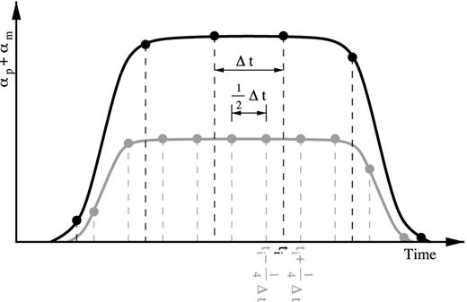
Schematic diagram showing αp + αm, the photon deficit due to the transit of the planet and the moon as a function of time, for two different exposure times. The long exposure time (black) is twice as long as the short exposure time (grey) and the exposures are indicated by vertical dashed lines. Note that the black curve is approximately twice as high as the grey curve as approximately twice as many photons are collected during the longer exposure.
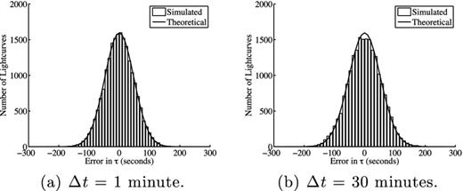
Comparison between results of the Monte Carlo simulation described in Section 3 for two different values of the exposure time. For these simulations it was assumed that the transit ingress and egress both lasted 1 hr, that the transit duration, Ttra, was 13 h, that the observing duration, Tobs, was 24 h and that σL was 0.54 and 0.10 times the transit depth for the case of 1 and 30 min exposures, respectively.
