A first-order secular theory for the post-Newtonian two-body problem with spin – I. The restricted case

Biscani, Francesco; Carloni, Sante

doi:10.1093/mnras/sts198

Abstract

We revisit the relativistic restricted two-body problem with spin employing a perturbation scheme based on Lie series. Starting from a post-Newtonian expansion of the field equations, we develop a first-order secular theory that reproduces well-known relativistic effects such as the precession of the pericentre and the Lense–Thirring and geodetic effects. Additionally, our theory takes into full account the complex interplay between the various relativistic effects, and provides a new explicit solution of the averaged equations of motion in terms of elliptic functions. Our analysis reveals the presence of particular configurations for which non-periodical behaviour can arise. The application of our results to real astrodynamical systems (such as Mercury-like and pulsar planets) highlights the contribution of relativistic effects to the long-term evolution of the spin and orbit of the secondary body.

gravitation, celestial mechanics

1 INTRODUCTION

The General Theory of Relativity (GR) has been one of the greatest achievements of the 20th century. Its formulation has revolutionized our way to understand the physical Universe and has led to the (sometimes unexpected) opening of entirely new research fields. One striking example is the formulation of a consistent theory describing the global behaviour of the Universe, which was impossible in the framework of Newtonian mechanics (Peebles 1993).

In Einstein's theory, the space–time is thought of as a four-dimensional pseudo-Riemannian manifold whose geometry interacts non-linearly with matter. Because of this feature, general calculations in GR require much more work than the corresponding ones in Newtonian gravity and this fact has made more difficult the understanding of the physics of Einsteinian gravity.

Another consequence of this difficulty falls in the context of testing Einstein's gravity: our inability to solve in general the gravitational field equations limits the possibility of devising full tests of GR. Instead, most of the investigation on the validity of this theory was performed in a regime of weak field leaving the strong-field regime almost completely unexplored.¹ In fact, all the tests of GR performed up to now belong to the class of weak-field experiments, from the so-called ‘classical tests’ of GR (Peebles 1993) to the latest tests based, for example, on the motion of interplanetary probes (Hees et al. 2011).

Einstein himself was well aware of the fact that the understanding of his theory in the perturbative regime was crucial for its testing and its application to the problems in which Newtonian gravity was most successful. For this reason in the 1930s he developed a perturbative approach able to describe the subtle changes induced on the Newtonian evolution of the bodies in the Solar system by General Relativity. The so-called Einstein–Infeld–Hoffman equations are the results at the first post-Newtonian level of this attempt (Einstein, Infeld & Hoffmann 1938).² The derivation of these equations was the birth of a new field called ‘Relativistic Celestial Mechanics’ (RCM; Brumberg 1991; Kopeikin, Efroimsky & Kaplan 2011).

The research in RCM has not stopped since then. The post-Newtonian equations have been analysed in many different ways and new and more powerful approaches to RCM have been proposed (see Damour, Soffel & Xu 1991a,b, 1993, 1994). In spite of these advances, the resolution of the post-Newtonian equations still remains a formidable task. In particular, the interaction between orbital and rotational motion has not been fully solved analytically to this date.

In this paper, we will focus on the post-Newtonian equations for a restricted two-spinning-body system at the 1PN level. Our target is to obtain a complete description of the leading correction of GR on Newtonian mechanics with a specific focus on the spin interaction effects. Such a target will be accomplished using modern perturbative methods based on Lie series (Hori 1966; Deprit 1969). This approach allows us to derive a fully analytical description of the long-term dynamical evolution of the system using semi-automatized computer algebra. Advantages of the Lie series procedure over traditional perturbation techniques include the availability of explicit formulae to convert between the averaged and non-averaged orbital elements, and the possibility to straightforwardly extend the treatment to higher post-Newtonian orders. Using the Lie series technique, we will re-derive the standard precession effects typical of the restricted two-body problem in General Relativity, but we will also give new analytical relations describing the evolution of spin and orbital angular momentum of the secondary body. In fact, we will be able to explore the full evolution of the orbital parameters of the secondary body and to quantify the effect of the spin–orbit and spin–spin interactions.

The use of the Lie series technique in RCM is relatively sparse, and, as far as we have been able to verify, it constitutes by itself a novelty in the analysis of relativistic spin–spin and spin–orbit interactions.³ In this first paper of the series, we have thus chosen to focus on the restricted problem in order to lay the foundation of our method in the simplest case of interest. In subsequent publications, we will tackle the full post-Newtonian two-body problem with spin building on the formalism introduced in this paper.

2 HAMILTONIAN FORMULATION

The starting point of our derivation is the well-known 1PN Hamiltonian of the two-body problem with spin, which, after reduction to the centre-of-mass frame, reads (Barker & O'Connell 1970, 1979; Damour 2001)

\begin{equation} \mathcal {H} = \mathcal {H}_{\rm N} + \epsilon \mathcal {H}_1. \end{equation}

(1)

Here ϵ = 1/c² is chosen as the ‘smallness parameter’ of our perturbation theory and

\begin{equation} \mathcal {H}_{\rm N} = \frac{1}{2}\frac{\boldsymbol {J}_1^2}{I_1} + \frac{1}{2}\frac{\boldsymbol {J}_2^2}{I_2} + \frac{\boldsymbol {p}^2}{2\mu }-\frac{\mathcal {G}M\mu }{r} \end{equation}

(2)

is the Newtonian Hamiltonian (representing the unperturbed problem). |$\mathcal {H}_1$| expands as

\begin{equation} \mathcal {H}_1 = \mathcal {H}_{\rm PN}+\mathcal {H}_{\rm SO}+\mathcal {H}_{\rm SS}, \end{equation}

(3)

where

\begin{eqnarray} \mathcal {H}_{\rm PN} &=& \mu \left\lbrace \frac{1}{8}\left( 3\nu -1\right)\frac{\boldsymbol {p}^4}{\mu ^4} {\left. -\frac{\mathcal {G}M}{2r}\left[\left(3+\nu \right)\frac{\boldsymbol {p}^2}{\mu ^2}+\nu \left(\boldsymbol {n}\cdot \frac{\boldsymbol {p}}{\mu }\right)^2\right] +\frac{\mathcal {G}^2M^2}{2r^2} \right\rbrace } \right.\nonumber \\ &&\left. -\frac{\mathcal {G}M}{2r}\left[\left(3+\nu \right)\frac{\boldsymbol {p}^2}{\mu ^2}+\nu \left(\boldsymbol {n}\cdot \frac{\boldsymbol {p}}{\mu }\right)^2\right] +\frac{\mathcal {G}^2M^2}{2r^2} \right\rbrace \end{eqnarray}

(4)

is the post-Newtonian orbital Hamiltonian,

\begin{eqnarray} \mathcal {H}_{\rm SO} = \frac{2\mathcal {G}}{r^3}\left[\left(1+\frac{3}{4}\frac{m_2}{m_1} \right)\boldsymbol {J}_1 + \left(1+\frac{3}{4}\frac{m_1}{m_2} \right)\boldsymbol {J}_2\right]\cdot \left(\boldsymbol {r}\times \boldsymbol {p}\right)\nonumber\\ \end{eqnarray}

(5)

represents the spin–orbit interaction, and

\begin{equation} \mathcal {H}_{\rm SS} = \frac{\mathcal {G}}{r^3}\left[3\left(\boldsymbol {J}_1\cdot \boldsymbol {n}\right)\left(\boldsymbol {J}_2\cdot \boldsymbol {n}\right)-\boldsymbol {J}_1\cdot \boldsymbol {J}_2\right] \end{equation}

(6)

represents the spin–spin coupling. In these formulae, |$\mathcal {G}$| is the universal gravitational constant, m₁ and m₂ are the masses of the two bodies, M = m₁ + m₂, μ = m₁m₂/M is the reduced mass, ν = μ/M, |$\boldsymbol {p}=\boldsymbol {p}_1=-\boldsymbol {p}_2$| is the canonical momentum of body 1, and |$\boldsymbol {r}=r\boldsymbol {n}$| is the vector connecting body 2 to body 1. The structure of this Hamiltonian and, above all, the nature of the spin vectors, has been a matter of debate in the past few years (see Damour, Jaranowski & Schäfer 2008). More recently, Wu & Xie (2010) have proposed a symplectic formulation of the spin vectors in terms of cylindrical-like coordinates. Here, we follow the interpretation of Barker & O'Connell (1975, 1976, 1979) and Wex (1995) in identifying the spins |$\boldsymbol {J}_i$| as the rotational angular momenta of spherical rigid bodies, so that

\begin{equation} \boldsymbol {J}_i = I_i\boldsymbol {\omega }_i, \end{equation}

(7)

where I_i is the moment of inertia and |$\boldsymbol {\omega }_i$| is the rotational angular velocity vector of body i.

In the present formulation of the Hamiltonian, we have dropped from |$\mathcal {H}_{{\rm SS}}$| the spin-quadratic contributions due to monopole–quadrupole interaction⁴ to focus on the leading relativistic effects. Besides, as pointed out by Damour (2001), at this PN order we can expect to obtain physically reliable results in the case of moderate spins and orbital velocities.

The equations of motion generated by equation (1) can be obtained via the familiar Hamiltonian canonical equations. The orbital momenta and coordinates are represented, respectively, by |$\boldsymbol {p}$| and |$\boldsymbol {r}$|⁠; the spin coordinates and momenta are represented by the Euler angles and their conjugate generalized momenta in terms of which the components of the angular velocities |$\boldsymbol {\omega }_i$| are expressed. At this stage, we are not concerned with the exact functional form of such dependence, as we will introduce a more convenient set of variables in Section 3. We refer to Gurfil et al. (2007) for a derivation of the Hamiltonian formulation of rigid-body dynamics.

The reduction of Hamiltonians (2)–(6) to the restricted case in which m₂ ≫ m₁ and |$\left|\boldsymbol {J}_2\right| \gg \left|\boldsymbol {J}_1\right|$| reads

\begin{eqnarray} \mathcal {H}_{\rm N} &=& \frac{1}{2}\frac{\boldsymbol {J}_1^2}{I_1} + \frac{\boldsymbol {p}_1^2}{2m_1}-\frac{\mathcal {G}m_1m_2}{r},\nonumber\\ \mathcal {H}_{\rm PN} &=& m_1\left( -\frac{1}{8}\frac{\boldsymbol {p}_1^4}{m_1^4} - \frac{3}{2}\frac{\mathcal {G}m_2}{r}\frac{\boldsymbol {p}_1^2}{m_1^2} +\frac{\mathcal {G}^2m_2^2}{2r^2} \right),\nonumber \\ \mathcal {H}_{\rm SO} &=& \frac{2\mathcal {G}}{r^3}\left(\frac{3}{4}\frac{m_2}{m_1}\boldsymbol {J}_1 + \boldsymbol {J}_2\right)\cdot \left(\boldsymbol {r}\times \boldsymbol {p}_1\right),\nonumber\\ \mathcal {H}_{\rm SS} &=& \frac{\mathcal {G}}{r^3}\left[3\left(\boldsymbol {J}_1\cdot \boldsymbol {n}\right)\left(\boldsymbol {J}_2\cdot \boldsymbol {n}\right)-\boldsymbol {J}_1\cdot \boldsymbol {J}_2\right], \end{eqnarray}

(8)

where |$\boldsymbol {J}_2$| is now considered as a constant of motion that can be dropped from |$\mathcal {H}_{\rm N}$|⁠. Without loss of generality, we can orient the reference system (now centred on body 2) in such a way that the constant |$\boldsymbol {J}_2$| is aligned to the positive z-axis, so that

\begin{equation} \boldsymbol {J}_2 = \left(0,0,J_2\right), \end{equation}

(9)

with |$J_2=\left| \boldsymbol {J}_2 \right|$|⁠.

3 ACTION-ANGLE VARIABLES

In preparation for the application of the Lie series perturbative approach in the study of Hamiltonian (8), we want to express the Hamiltonian in a coordinate system of action-angle variables (Arnold 1989) for the unperturbed problem. For the orbital variables, a common choice is the set of Delaunay elements (Morbidelli 2002). For the rotational motion, a suitable choice in our case is that of Serret–Andoyer (SA) variables (Gurfil et al. 2007). Both sets of variables are introduced formally as canonical transformations.

Before proceeding, we need to discuss briefly the nature of the canonical momenta appearing in Hamiltonian (8). Post-Newtonian Hamiltonians are derived from Lagrangians in which the generalized velocities appear not only in the kinetic terms of the Newtonian portion of the Lagrangian, but also in the relativistic perturbation (see e.g. Landau & Lifschits 1975; Straumann 1984). As a consequence, after switching to the Hamiltonian formulation via the usual Legendre transformation procedure, the post-Newtonian canonical Hamiltonian momenta will differ from the Newtonian ones by terms of order 1/c². This discrepancy will carry over to any subsequent canonical transformation, including the introduction of Delaunay and SA elements. Richardson & Kelly (1988) and Heimberger et al. (1990) analyse in detail the connection between Newtonian and post-Newtonian Delaunay orbital elements.

However, in this work, we are concerned with the secular variations of orbital and rotational elements, for which the discrepancy discussed above is of little consequence. For if a secular motion (e.g. a precession of the node) results from our analysis in terms of post-Newtonian elements, it will affect within an accuracy of 1/c² also the Newtonian elements.⁵ Indeed, we will show how our analysis in terms of post-Newtonian elements reproduces exactly the formulae of known secular relativistic effects.

3.1 Delaunay elements

The Delaunay arguments (L, G, H, l, g, h) can be introduced via the following standard relations (Morbidelli 2002):

\begin{equation} \begin{array}{@{}l@{\quad}c@{}} L = \sqrt{\mathcal {G}m_{2}a}, & l = M,\\ G = L\sqrt{1-e^{2}}, & g = \omega ,\\ H = G\cos i, & h = \Omega .\\ \end{array} \end{equation}

(10)

Here a, e, i, M, ω and Ω are the classical Keplerian orbital elements describing the trajectory of the secondary body m₁ around the primary m₂. The Keplerian elements are in turn related to the Cartesian orbital momentum |$\boldsymbol {p}_1$| and position |$\boldsymbol {r}$| via well-known relations (e.g. see Murray & Dermott 2000). In equations (10), (L, G, H) play the role of generalized momenta; (l, g, h) are the generalized coordinates.

3.2 Serret–Andoyer variables

The SA variables describe the rotational motion of a rigid body in terms of orientation angles and rotational angular momenta. In our specific case, the bodies are perfectly spherical and thus the introduction of SA elements is simplified with respect to the general case. We refer to Gurfil et al. (2007) for an exhaustive treatment of the SA formalism in the general case.

We start by expressing |$\boldsymbol {J}_1$| in a coordinate system where |$\boldsymbol {J}_1$| itself is aligned to the z-axis, so that |$\boldsymbol {J}_1=\left(0,0,\left|\boldsymbol {J}_{1}\right|\right)$|⁠.⁶ In order to express the components of |$\boldsymbol {J}_1$| in the centre-of-mass reference system, we compose two rotations: the first one around the x-axis by −I (the inclination of |$\boldsymbol {J}_1$|⁠), the second one around the new z-axis by |$-\tilde{h}$| (the nodal angle of |$\boldsymbol {J}_1$|⁠, analogous to the h angle in the Delaunay element set or to the longitude of the node in the set of Keplerian elements), resulting in the composite rotation matrix

\begin{equation} \left[\begin{array}{@{}c@{\quad}c@{\quad}c@{}}\cos \tilde{h} & -\sin \tilde{h}\cos I & \sin I\sin \tilde{h}\\ \sin \tilde{h} & \cos I\cos \tilde{h} & -\sin I\cos \tilde{h}\\ 0 & \sin I & \cos I \end{array}\right]. \end{equation}

(11)

In the SA formalism, |$\cos I=J_{1,z} / \left|\boldsymbol {J}_1\right|$| (where J_{1, z} is the z-component of the rotational angular momentum in the centre-of-mass reference system). Thus, in the centre-of-mass reference system, the components of |$\boldsymbol {J}_1$| read

\begin{equation} \boldsymbol {J}_1=\left(\sqrt{\left|\boldsymbol {J}_1\right|^2-J_{1,z}^2}\sin \tilde{h}, -\sqrt{\left|\boldsymbol {J}_1\right|^2-J_{1,z}^2}\cos \tilde{h},J_{1,z}\right). \end{equation}

(12)

In the SA variable set, |$\left(\left|\boldsymbol {J}_1\right|,J_{1,z}\right)$| are the generalized momenta, and |$\left(\tilde{g},\tilde{h}\right)$| are the conjugate coordinates. Note that due to the spherical symmetry of the bodies, the angle |$\tilde{g}$| conjugated to the action |$\left|\boldsymbol {J}_1\right|$| does not appear in the expression of the Hamiltonian and |$\left|\boldsymbol {J}_1\right|$| is thus conserved.

3.3 Final form of the Hamiltonian

We are now ready to express Hamiltonian (8) in terms of Delaunay and SA arguments. Before proceeding to the substitutions, in order to simplify the notation, we rescale the Hamiltonian via an extended canonical transformation, dividing the Hamiltonian and the generalized momenta by m₁. The resulting expressions for |$\mathcal {H}_{\rm N}$| and |$\mathcal {H}_1$| in terms of the momenta |$\left(L,G,H,\tilde{G},\tilde{H}\right)$| and coordinates |$\left(l,g,h,\tilde{g},\tilde{h}\right)$| read

\begin{eqnarray} \mathcal {H}_{{\rm N}}& = \frac{1}{2}\mathcal {I}_{1}\tilde{G}^{2}-\displaystyle\frac{\mathcal {G}^{2}m_{2}^{2}}{2L^{2}}, \end{eqnarray}

(13)

\begin{eqnarray} \mathcal {H}_{1} &=& -\,\frac{1}{8}\frac{\mathcal {G}^{4}m_{2}^{4}}{L^{4}}+\frac{1}{r}\frac{2\mathcal {G}^{3}m_{2}^{3}}{L^{2}}-\frac{1}{r^{2}}3\mathcal {G}^{2}m_{2}^{2}\nonumber \\ && +\,\frac{\mathcal {G}}{r^{3}}\left\lbrace 2J_{2}H+\frac{3J_{2}G_{xy}^{2}\tilde{H}}{2G^{2}}+\frac{3m_{2}\tilde{H}H}{2}-J_{2}\tilde{H}\right.\nonumber \\ && +\,\left(\frac{3m_{2}}{2}\tilde{G}_{xy}G_{xy}-\frac{3}{2}J_{2}\frac{HG_{xy}\tilde{G}_{xy}}{G^{2}}\right)\cos \left(\tilde{h}-h\right)\nonumber \\ && +\,3J_{2}\left[-\frac{1}{2}\frac{G_{xy}^{2}\tilde{H}}{G^{2}}\cos \left(2f+2g\right)\right.\nonumber \\ && -\,\frac{1}{4}\frac{G_{xy}\tilde{G}_{xy}}{G}\left(1-\frac{H}{G}\right)\cos \left(2f+2g+\tilde{h}-h\right)\nonumber \\ && +\left.\left.{\frac{3J_{2}G_{xy}^{2}\tilde{H}}{2G^{2}}}\!\! \frac{1}{4}\frac{G_{xy}\tilde{G}_{xy}}{G}\left(1+\frac{H}{G}\right)\cos \left(2f+2g-\tilde{h}+h\right)\right]\right\rbrace . \end{eqnarray}

(14)

For convenience, we have summarized in Table 1 the meaning of the symbolic variables appearing in Hamiltonians (13) and (14). We have to stress how in these expressions, r, G_xy, |$\tilde{G}_{xy}$| and f have to be regarded as implicit functions of the canonical momenta and coordinates. Specifically,

\begin{eqnarray} r &=& r\left(L,G,l\right), \end{eqnarray}

(15)

\begin{eqnarray} G_{xy} &=& G_{xy}\left(G,H\right), \end{eqnarray}

(16)

\begin{eqnarray} \tilde{G}_{xy} &=& \tilde{G}_{xy}\left(\tilde{G},\tilde{H}\right), \end{eqnarray}

(17)

\begin{eqnarray} f &=& f\left(L,G,l\right). \end{eqnarray}

(18)

We are now ready to analyse the Hamiltonian using the Lie series method.

Table 1.

Summary and explanation of the symbolic variables appearing in Hamiltonians (13) and (14).

Symbol	Meaning	Alternative expression
L	Normalized square root of the semi-major axis	\|$\sqrt{\mathcal {G}m_{2}a}$\|
G	Norm of the orbital angular momentum \|$\boldsymbol {r}\times \boldsymbol {p}_1$\| normalized by m₁	\|$L\sqrt{1-e^2}$\|
H	z-component of the orbital angular momentum normalized by m₁	G cos i
\|$\tilde{G}$\|	Norm of spin \|$\boldsymbol {J}_1$\| normalized by m₁	\|$\left\|\boldsymbol {J}_1\right\|/m_1$\|
\|$\tilde{H}$\|	z-component of spin \|$\boldsymbol {J}_1$\| normalized by m₁	\|$\tilde{G}\cos {I}$\|
l	Mean anomaly	M
g	Argument of pericentre	ω
h	Longitude of the ascending node	Ω
\|$\tilde{h}$\|	Nodal angle of spin \|$\boldsymbol {J}_1$\|	–
f	True anomaly	–
\|$\mathcal {I}_1$\|	Inverse of the moment of inertia of body 1 normalized by m₁	m₁/I₁
G_xy	Norm of the projection of \|$\boldsymbol {r}\times \boldsymbol {p}_1$\| on the xy-plane normalized by m₁	\|$\sqrt{G^2-H^2}$\|
\|$\tilde{G}_{xy}$\|	Norm of the projection of spin \|$\boldsymbol {J}_1$\| on the xy-plane normalized by m₁	\|$\sqrt{\tilde{G}^2-\tilde{H}^2}$\|
J₂	Norm of spin \|$\boldsymbol {J}_2$\|	\|$\left\|\boldsymbol {J}_2\right\|$\|
r	Distance between body 1 and body 2	–
m₁, m₂	Masses of the two bodies	–
\|$\mathcal {G}$\|	Universal gravitational constant	–

Symbol	Meaning	Alternative expression
L	Normalized square root of the semi-major axis	\|$\sqrt{\mathcal {G}m_{2}a}$\|
G	Norm of the orbital angular momentum \|$\boldsymbol {r}\times \boldsymbol {p}_1$\| normalized by m₁	\|$L\sqrt{1-e^2}$\|
H	z-component of the orbital angular momentum normalized by m₁	G cos i
\|$\tilde{G}$\|	Norm of spin \|$\boldsymbol {J}_1$\| normalized by m₁	\|$\left\|\boldsymbol {J}_1\right\|/m_1$\|
\|$\tilde{H}$\|	z-component of spin \|$\boldsymbol {J}_1$\| normalized by m₁	\|$\tilde{G}\cos {I}$\|
l	Mean anomaly	M
g	Argument of pericentre	ω
h	Longitude of the ascending node	Ω
\|$\tilde{h}$\|	Nodal angle of spin \|$\boldsymbol {J}_1$\|	–
f	True anomaly	–
\|$\mathcal {I}_1$\|	Inverse of the moment of inertia of body 1 normalized by m₁	m₁/I₁
G_xy	Norm of the projection of \|$\boldsymbol {r}\times \boldsymbol {p}_1$\| on the xy-plane normalized by m₁	\|$\sqrt{G^2-H^2}$\|
\|$\tilde{G}_{xy}$\|	Norm of the projection of spin \|$\boldsymbol {J}_1$\| on the xy-plane normalized by m₁	\|$\sqrt{\tilde{G}^2-\tilde{H}^2}$\|
J₂	Norm of spin \|$\boldsymbol {J}_2$\|	\|$\left\|\boldsymbol {J}_2\right\|$\|
r	Distance between body 1 and body 2	–
m₁, m₂	Masses of the two bodies	–
\|$\mathcal {G}$\|	Universal gravitational constant	–

Open in new tab

Table 1.

Summary and explanation of the symbolic variables appearing in Hamiltonians (13) and (14).

Symbol	Meaning	Alternative expression
L	Normalized square root of the semi-major axis	\|$\sqrt{\mathcal {G}m_{2}a}$\|
G	Norm of the orbital angular momentum \|$\boldsymbol {r}\times \boldsymbol {p}_1$\| normalized by m₁	\|$L\sqrt{1-e^2}$\|
H	z-component of the orbital angular momentum normalized by m₁	G cos i
\|$\tilde{G}$\|	Norm of spin \|$\boldsymbol {J}_1$\| normalized by m₁	\|$\left\|\boldsymbol {J}_1\right\|/m_1$\|
\|$\tilde{H}$\|	z-component of spin \|$\boldsymbol {J}_1$\| normalized by m₁	\|$\tilde{G}\cos {I}$\|
l	Mean anomaly	M
g	Argument of pericentre	ω
h	Longitude of the ascending node	Ω
\|$\tilde{h}$\|	Nodal angle of spin \|$\boldsymbol {J}_1$\|	–
f	True anomaly	–
\|$\mathcal {I}_1$\|	Inverse of the moment of inertia of body 1 normalized by m₁	m₁/I₁
G_xy	Norm of the projection of \|$\boldsymbol {r}\times \boldsymbol {p}_1$\| on the xy-plane normalized by m₁	\|$\sqrt{G^2-H^2}$\|
\|$\tilde{G}_{xy}$\|	Norm of the projection of spin \|$\boldsymbol {J}_1$\| on the xy-plane normalized by m₁	\|$\sqrt{\tilde{G}^2-\tilde{H}^2}$\|
J₂	Norm of spin \|$\boldsymbol {J}_2$\|	\|$\left\|\boldsymbol {J}_2\right\|$\|
r	Distance between body 1 and body 2	–
m₁, m₂	Masses of the two bodies	–
\|$\mathcal {G}$\|	Universal gravitational constant	–

Symbol	Meaning	Alternative expression
L	Normalized square root of the semi-major axis	\|$\sqrt{\mathcal {G}m_{2}a}$\|
G	Norm of the orbital angular momentum \|$\boldsymbol {r}\times \boldsymbol {p}_1$\| normalized by m₁	\|$L\sqrt{1-e^2}$\|
H	z-component of the orbital angular momentum normalized by m₁	G cos i
\|$\tilde{G}$\|	Norm of spin \|$\boldsymbol {J}_1$\| normalized by m₁	\|$\left\|\boldsymbol {J}_1\right\|/m_1$\|
\|$\tilde{H}$\|	z-component of spin \|$\boldsymbol {J}_1$\| normalized by m₁	\|$\tilde{G}\cos {I}$\|
l	Mean anomaly	M
g	Argument of pericentre	ω
h	Longitude of the ascending node	Ω
\|$\tilde{h}$\|	Nodal angle of spin \|$\boldsymbol {J}_1$\|	–
f	True anomaly	–
\|$\mathcal {I}_1$\|	Inverse of the moment of inertia of body 1 normalized by m₁	m₁/I₁
G_xy	Norm of the projection of \|$\boldsymbol {r}\times \boldsymbol {p}_1$\| on the xy-plane normalized by m₁	\|$\sqrt{G^2-H^2}$\|
\|$\tilde{G}_{xy}$\|	Norm of the projection of spin \|$\boldsymbol {J}_1$\| on the xy-plane normalized by m₁	\|$\sqrt{\tilde{G}^2-\tilde{H}^2}$\|
J₂	Norm of spin \|$\boldsymbol {J}_2$\|	\|$\left\|\boldsymbol {J}_2\right\|$\|
r	Distance between body 1 and body 2	–
m₁, m₂	Masses of the two bodies	–
\|$\mathcal {G}$\|	Universal gravitational constant	–

Open in new tab

4 PERTURBATION THEORY VIA LIE SERIES

The Lie series perturbative methodology (Hori 1966; Deprit 1969) aims at simplifying the Hamiltonian of the problem via a quasi-identity canonical transformation of coordinates depending on a generating function χ to be determined. The Lie series transformation reads

\begin{equation} \mathcal {H}^{\prime }=\mathcal {S}_{\chi }^{\epsilon }\mathcal {H}=\sum _{n=0}^\infty \frac{\epsilon ^{n}}{n!}\mathcal {L}_{\chi }^{n}\mathcal {H}, \end{equation}

(19)

where |$\mathcal {L}_{\chi }^{n}$| is the Lie derivative of nth order with generator χ, |$\mathcal {H}^{\prime }$| is the transformed Hamiltonian, and |$\mathcal {H}$| is the original Hamiltonian in which the new momenta and coordinates have been formally substituted. At the first order in ϵ the Lie derivative degenerates to a Poisson bracket, and the transformation becomes

\begin{equation} \mathcal {H}^{\prime }=\mathcal {H}_{\rm N}+\epsilon \underbrace{\left(\left\lbrace \mathcal {H}_{\rm N},\chi \right\rbrace +\mathcal {H}_{1}\right)}_{\mathcal {K}}+{\rm O}\left(\epsilon ^2\right). \end{equation}

(20)

We need then to solve the homological equation (Arnold 1989)

\begin{equation} \left\lbrace \mathcal {H}_{\rm N},\chi \right\rbrace +\mathcal {H}_{1}=\mathcal {K}, \end{equation}

(21)

where χ and |$\mathcal {K}$| (the new perturbed Hamiltonian resulting from the transformation of coordinates) have to be determined with the goal of obtaining some form of simplification in |$\mathcal {K}$|⁠. Since the unperturbed Hamiltonian depends only on the two actions L and |$\tilde{G}$|⁠, we have

\begin{equation} \left\lbrace \mathcal {H}_{\rm N},\chi \right\rbrace =-\frac{\mathrm{\partial} \mathcal {H}_{\rm N}}{\mathrm{\partial} L}\frac{\mathrm{\partial} \chi }{\mathrm{\partial} l} =-\frac{\mathcal {G}^{2}m_{2}^{2}}{L^{3}}\frac{\mathrm{\partial} \chi }{\mathrm{\partial} l}, \end{equation}

(22)

where the partial derivative of χ with respect to |$\tilde{g}$| (the coordinate conjugated to |$\tilde{G}$|⁠) can be set to zero as |$\tilde{G}$| is a constant of motion. The homological equation (21) then reads

\begin{equation} \chi =\int \frac{L^{3}}{\mathcal {G}^{2}m_{2}^{2}}\left(\mathcal {H}_{1}-\mathcal {K}\right){\rm d}l. \end{equation}

(23)

The technical aspects of the solution of this integral, including the choice of |$\mathcal {K}$|⁠, are detailed in Appendix A. Here we will limit ourselves to the following considerations:

The integral in equation (23) essentially represents an averaging over the mean motion l. Consequently, the new momenta and coordinates generated by the Lie series transformation are the mean counterparts of the original momenta and coordinates.
Thanks to the functional form of Hamiltonians (13) and (14), the averaging procedure removes at the same time both l and g from the averaged Hamiltonian.
The integration is performed in closed form, that is, without resorting to Fourier–Taylor expansions in terms of mean anomaly and eccentricity (Deprit 1982; Palacián 2002). The results are thus valid also for highly eccentric orbits.

The computations involved in the averaging procedure have been carried out with the Piranha computer algebra system (Biscani 2008). As usual when operating with Lie series transformations, from now on we will refer to the mean momenta and coordinates |$\left(L^\prime ,G^\prime ,H^\prime ,\tilde{G}^\prime ,\tilde{H}^\prime \right)$| and |$\left(l^\prime ,g^\prime ,h^\prime ,\tilde{g}^\prime ,\tilde{h}^\prime \right)$| with their original names |$\left(L,G,H,\tilde{G},\tilde{H}\right)$| and |$\left(l,g,h,\tilde{g},\tilde{h}\right)$|⁠, respectively, in order to simplify the notation.

After having determined χ from equation (23), the averaged Hamiltonian generated by equation (21) reads, in terms of mean elements,

\begin{equation} \mathcal {H}^{\prime }=\mathcal {H}_{\rm N}+\epsilon \left[\mathcal {E}_{0}+\mathcal {E}_{1}\cos \left(\tilde{h}-h\right)\right], \end{equation}

(24)

where |$\mathcal {E}_{0}$| and |$\mathcal {E}_{1}$| are functions of the mean momenta only. In order to further reduce the number of degrees of freedom, we perform a final canonical transformation⁷ that compresses the coordinates h and |$\tilde{h}$| in a single coordinate h_* (replacing h) and introduces a new momentum |$\tilde{H}_{\ast }$| (replacing |$\tilde{H}$|⁠) via the relations

\begin{eqnarray} \tilde{H}_{\ast } &=& H+\tilde{H}, \end{eqnarray}

(25)

\begin{eqnarray} h_{\ast } &=& h-\tilde{h}. \end{eqnarray}

(26)

After this transformation, the final averaged Hamiltonian reads

\begin{equation} \mathcal {H}^{\prime }=\mathcal {H}_{\rm N}+\epsilon \left(\mathcal {F}_{0}+\mathcal {F}_{1}\cos h_\ast \right), \end{equation}

(27)

where |$\mathcal {F}_{0}$| and |$\mathcal {F}_{1}$| are functions of the mean momenta only,

\begin{eqnarray} \mathcal {F}_{0} &=& \frac{1}{2}\frac{{J_2}{\mathcal {G}}^{4}{\tilde{H}_\ast }{m_2}^{3}}{{G}^{3}{L}^{3}} +\frac{3}{2}\frac{{H}^{3}{J_2}{\mathcal {G}}^{4}{m_2}^{3}}{{G}^{5}{L}^{3}}+\frac{15}{8}\frac{{\mathcal {G}}^{4}{m_2}^{4}}{{L}^{4}}\nonumber \\ && +\,\frac{3}{2}\frac{{H}{J_2}{\mathcal {G}}^{4}{m_2}^{3}}{{G}^{3}{L}^{3}}-\frac{3}{2}\frac{{H}^{2}{J_2}{\mathcal {G}}^{4}{\tilde{H}_\ast }{m_2}^{3}}{{G}^{5}{L}^{3}} -\frac{3}{2}\frac{{H}^{2}{\mathcal {G}}^{4}{m_2}^{4}}{{G}^{3}{L}^{3}}\nonumber \\ && +\,\frac{3}{2}\frac{{H}{\mathcal {G}}^{4}{\tilde{H}_\ast }{m_2}^{4}}{{G}^{3}{L}^{3}}-3\frac{{\mathcal {G}}^{4}{m_2}^{4}}{{G}{L}^{3}}, \end{eqnarray}

(28)

\begin{eqnarray} \mathcal {F}_{1} &=& -\frac{3}{2}\frac{{G_{xy}}{H}{J_2}{\mathcal {G}}^{4}{\tilde{G}_{xy\ast }}{m_2}^{3}}{{G}^{5}{L}^{3}}+\frac{3}{2}\frac{{G_{xy}}{\mathcal {G}}^{4}{\tilde{G}_{xy\ast }}{m_2}^{4}}{{G}^{3}{L}^{3}}, \end{eqnarray}

(29)

and |$\tilde{G}_{xy\ast }$| is the mean |$\tilde{G}_{xy}$| (see Table 1) expressed in terms of the new mean momentum |$\tilde{H}_{\ast }$|⁠:

\begin{equation} \tilde{G}_{xy\ast }=\sqrt{\tilde{G}^{2}-\left(\tilde{H}_{\ast }-H\right)^{2}}. \end{equation}

(30)

We are now ready to proceed to an analysis of the averaged Hamiltonian (27).

5 ANALYSIS OF THE AVERAGED HAMILTONIAN

5.1 Preliminary considerations

The 1 degree-of-freedom averaged Hamiltonian (27) is expressed in terms of the mean momenta |$\left(L,G,H,\tilde{G},\tilde{H}_\ast \right)$| and conjugate mean coordinates |$\left(l,g,h_\ast ,\tilde{g},\tilde{h}\right)$|⁠. The equations of motion generated by Hamiltonian (27) read

\begin{eqnarray} \frac{{\rm d}L}{{\rm d}t} &=& 0,\nonumber\\ \frac{{\rm d}G}{{\rm d}t} &=& 0,\nonumber\\ \frac{{\rm d}H}{{\rm d}t} &=& \epsilon \mathcal {F}_{1}\sin h_{\ast },\nonumber\\ \frac{{\rm d}\tilde{G}}{{\rm d}t} &=& 0,\nonumber\\ \frac{{\rm d}\tilde{H}_{\ast }}{{\rm d}t} &=& 0, \end{eqnarray}

(31)

and

\begin{eqnarray} \frac{{\rm d}l}{{\rm d}t} &=& \frac{\mathcal {G}^{2}m_{2}^{2}}{L^{3}}+\epsilon \left(\frac{\mathrm{\partial} \mathcal {F}_{0}}{\mathrm{\partial} L}+\frac{\mathrm{\partial} \mathcal {F}_{1}}{\mathrm{\partial} L}\cos h_{\ast }\right),\nonumber\\ \frac{{\rm d}g}{{\rm d}t} &=& \epsilon \left(\frac{\mathrm{\partial} \mathcal {F}_{0}}{\mathrm{\partial} G}+\frac{\mathrm{\partial} \mathcal {F}_{1}}{\mathrm{\partial} G}\cos h_{\ast }\right),\nonumber\\ \frac{{\rm d}h_{\ast }}{{\rm d}t} &=& \epsilon \left(\frac{\mathrm{\partial} \mathcal {F}_{0}}{\mathrm{\partial} H}+\frac{\mathrm{\partial} \mathcal {F}_{1}}{\mathrm{\partial} H}\cos h_{\ast }\right),\nonumber\\ \frac{{\rm d}\tilde{g}}{{\rm d}t} &=& \mathcal {I}_{1}\tilde{G}+\epsilon \frac{\mathrm{\partial} \mathcal {F}_{1}}{\mathrm{\partial} \tilde{G}}\cos h_{\ast },\nonumber\\ \frac{{\rm d}\tilde{h}}{{\rm d}t} &=& \epsilon \left(\frac{\mathrm{\partial} \mathcal {F}_{0}}{\mathrm{\partial} \tilde{H}_{\ast }}+\frac{\mathrm{\partial} \mathcal {F}_{1}}{\mathrm{\partial} \tilde{H}_{\ast }}\cos h_{\ast }\right). \end{eqnarray}

(32)

A first straightforward consequence of the form of the averaged Hamiltonian is the conservation of all mean momenta apart from H. In particular, the conservation of the mean momentum |$\tilde{H}_\ast =H+\tilde{H}$| corresponds to the conservation of the z-component of the total mean angular momentum of the system. We refer the reader to Appendix B for the full functional form of the partial derivatives of |$\mathcal {F}_0$| and |$\mathcal {F}_1$| with respect to the mean momenta.

We are now going to proceed to the derivation of the well-known relativistic effect in a series of simplified cases of Hamiltonian (27).

5.2 Einstein precession

In this simplest case, all spin-related interactions are suppressed and only the classical 1PN orbital effects remain. Formally, the spin effects are suppressed by setting |$J_2=\tilde{G}=0$| and |$\tilde{H}_\ast = H$| in the equations of motion (31) and (32). We have to point out a formal difficulty in such a direct substitution, arising from the fact that when the spin |$\tilde{G}$| is suppressed the angles h_* and |$\tilde{h}$| become undefined and equations (B7)–(B9) have a pole in |$\tilde{G}_{xy\ast }=0$|⁠.⁸ In order to avoid these problems, we can write directly the equation of motion for |$h=\tilde{h}+h_\ast$| in the general case as

\begin{eqnarray} \frac{{\rm d}h}{{\rm d}t} &=& \frac{{\rm d}\tilde{h}}{{\rm d}t} + \frac{{\rm d} h_\ast }{{\rm d}t} \nonumber \\ &=& \epsilon \left[2\frac{{J_2}{\mathcal {G}}^{4}{m_2}^{3}}{{G}^{3}{L}^{3}} -3\frac{{H}{J_2}{\mathcal {G}}^{4}{\tilde{H}_\ast }{m_2}^{3}}{{G}^{5}{L}^{3}} -\frac{3}{2}\frac{{H}{\mathcal {G}}^{4}{m_2}^{4}}{{G}^{3}{L}^{3}}\right.\nonumber \\ &&+\,3\frac{{H}^{2}{J_2}{\mathcal {G}}^{4}{m_2}^{3}}{{G}^{5}{L}^{3}} +\frac{3}{2}\frac{{\mathcal {G}}^{4}{\tilde{H}_\ast }{m_2}^{4}}{{G}^{3}{L}^{3}}+\left(\frac{3}{2}\frac{{H}^{2}{J_2}{\mathcal {G}}^{4}{\tilde{G}_{xy\ast }}{m_2}^{3}}{{G}^{5}{G_{xy}}{L}^{3}}\right.\nonumber \\ &&-\left.\left.\!\frac{3}{2}\frac{{G_{xy}}{J_2}{\mathcal {G}}^{4}{\tilde{G}_{xy\ast }}{m_2}^{3}}{{G}^{5}{L}^{3}} -\frac{3}{2}\frac{{H}{\mathcal {G}}^{4}{\tilde{G}_{xy\ast }}{m_2}^{4}}{{G}^{3}{G_{xy}}{L}^{3}}\right)\cos {{h_\ast }}\right], \end{eqnarray}

(33)

and verify that this equation is regular in the absence of spins: the poles have disappeared and the the indeterminacy of h_* is inconsequential as the factor of cos h_* becomes zero in the absence of spins.

The equations of motion of the mean orbital coordinates in the absence of spins thus become

\begin{eqnarray} \frac{{\rm d}l}{{\rm d}t} &=& \frac{\mathcal {G}^{2}m_{2}^{2}}{L^{3}}+\epsilon \left(9\frac{{\mathcal {G}}^{4}{m_2}^{4}}{{G}{L}^{4}}-\frac{15}{2}\frac{{\mathcal {G}}^{4}{m_2}^{4}}{{L}^{5}}\right), \end{eqnarray}

(34)

\begin{eqnarray} \frac{{\rm d}g}{{\rm d}t} &=& 3\epsilon \frac{{\mathcal {G}}^{4}{m_2}^{4}}{{G}^{2}{L}^{3}}, \end{eqnarray}

(35)

\begin{eqnarray} \frac{{\rm d}h}{{\rm d}t} &=& 0, \end{eqnarray}

(36)

whereas all mean momenta are constants of motion. We can recognize in equation (35) the classical relativistic effect of the pericentre precession. In Keplerian orbital elements (see conversion formulae 10), equation (35) becomes

\begin{equation} \frac{{\rm d}g}{{\rm d}t}\equiv \frac{{\rm d}\omega }{{\rm d}t}=\frac{3m_{2}^{\frac{3}{2}}\mathcal {G}^{\frac{3}{2}}}{c^{2}a^{\frac{5}{2}}\left(1-e^{2}\right)}, \end{equation}

(37)

which, over an averaged orbit of the secondary body of period

\begin{equation} T=2\pi \sqrt{\frac{a^{3}}{m_{2}\mathcal {G}}}, \end{equation}

(38)

amounts to

\begin{equation} \Delta \omega =\frac{6\pi \mathcal {G}m_{2}}{c^{2}a\left(1-e^{2}\right)}, \end{equation}

(39)

which is the classical formula for the relativistic pericentre precession (Einstein 1916; Straumann 1984). The result for the perturbation on the mean anomaly l is in agreement with the results of Richardson & Kelly (1988) and Heimberger et al. (1990), also obtained with a Lie series technique.

5.3 Lense–Thirring effect

The case in which only the central body is spinning corresponds to J₂ ≠ 0, |$\tilde{G}=0$| and |$\tilde{H}_{\ast } = H$|⁠. As in the preceding case, all mean momenta are constants of motion, and the equations for the mean orbital coordinates become

\begin{eqnarray} \frac{{\rm d}l}{{\rm d}t} &=& \frac{\mathcal {G}^{2}m_{2}^{2}}{L^{3}}+\epsilon \left(9\frac{{\mathcal {G}}^{4}{m_2}^{4}}{{G}{L}^{4}}-6\frac{{H}{J_2}{\mathcal {G}}^{4}{m_2}^{3}}{{G}^{3}{L}^{4}}-\frac{15}{2}\frac{{\mathcal {G}}^{4}{m_2}^{4}}{{L}^{5}}\right), \end{eqnarray}

(40)

\begin{eqnarray} \frac{{\rm d}g}{{\rm d}t} &=& \epsilon \left(-6\frac{{H}{J_2}{\mathcal {G}}^{4}{m_2}^{3}}{{G}^{4}{L}^{3}}+3\frac{{\mathcal {G}}^{4}{m_2}^{4}}{{G}^{2}{L}^{3}}\right), \end{eqnarray}

(41)

\begin{eqnarray} \frac{{\rm d}h}{{\rm d}t} &=& 2\epsilon \frac{{J_2}{\mathcal {G}}^{4}{m_2}^{3}}{{G}^{3}{L}^{3}}. \end{eqnarray}

(42)

Here we can clearly recognize the effect of the interaction of the spin of the central body with the orbit of the (non-rotating) secondary body. This effect is sometimes referred to as Lense–Thirring precession (Thirring 1918). The equations above show that the consequence of endowing the central body with a spin is that of modifying Einstein's pericentre precession via the additional term

\begin{equation} -6\frac{{H}{J_2}{\mathcal {G}}^{4}{m_2}^{3}}{{G}^{4}{L}^{3}}, \end{equation}

(43)

and of introducing a precession of the mean line of nodes with angular velocity

\begin{equation} 2\frac{{J_2}{\mathcal {G}}^{4}{m_2}^{3}}{c^2{G}^{3}{L}^{3}}. \end{equation}

(44)

Both these formulae are in agreement with the results of Bogorodskii (1959) and Cugusi & Proverbio (1978).

5.4 Geodetic effect

The case in which only the secondary body is spinning corresponds to J₂ = 0 and |$\tilde{G}\ne 0$|⁠. This configuration is clearly more complicated than the previous two cases, as now |$\mathcal {F}_1\ne 0$| and the mean momentum H is not a constant of motion any more. The equations of motion for H and its conjugate mean coordinate h_* read

\begin{eqnarray} \frac{{\rm d}H}{{\rm d}t} &=& \frac{3}{2}\epsilon \frac{{G_{xy}}{\mathcal {G}}^{4}{\tilde{G}_{xy\ast }}{m_2}^{4}}{{G}^{3}{L}^{3}}\sin {h_\ast }, \end{eqnarray}

(45)

\begin{eqnarray} \frac{{\rm d}h_\ast }{{\rm d}t} &=& \epsilon \left[ -3\frac{{H}{\mathcal {G}}^{4}{m_2}^{4}}{{G}^{3}{L}^{3}} +\frac{3}{2}\frac{{\mathcal {G}}^{4}{\tilde{H}_\ast }{m_2}^{4}}{{G}^{3}{L}^{3}} +\left(-\frac{3}{2}\frac{{G_{xy}}{H}{\mathcal {G}}^{4}{m_2}^{4}}{{G}^{3}{L}^{3}{\tilde{G}_{xy\ast }}}\right.\right.\nonumber \\ &&\left.\left.+\frac{3}{2}\frac{{G_{xy}}{\mathcal {G}}^{4}{\tilde{H}_\ast }{m_2}^{4}}{{G}^{3}{L}^{3}{\tilde{G}_{xy\ast }}} -\frac{3}{2}\frac{{H}{\mathcal {G}}^{4}{\tilde{G}_{xy\ast }}{m_2}^{4}}{{G}^{3}{G_{xy}}{L}^{3}}\right)\cos {h_\ast }\right]. \end{eqnarray}

(46)

A first observation is that, since J₂ = 0, there is no preferred orientation for the reference system, and the form of the equations of motion is rotationally invariant. As an immediate consequence, the fact that the mean momentum |$\tilde{H}_\ast =H+\tilde{H}$| is constant regardless of the orientation of the reference system implies that in this case the total mean angular momentum vector is a constant of motion (whereas in the general case only its z-component is conserved). In turn, this observation, together with the conservation of the norms of the mean orbital and rotational angular momenta G and |$\tilde{G}$|⁠, respectively, implies that the only possible motion for the mean orbital and rotational angular momentum vectors is a simultaneous precession around the total mean angular momentum vector.

It is possible to verify this result and to quantify the precessional motion via a phase-space analysis. The dynamical system defined by equations (45) and (46) has three equilibrium points. The first one,

\begin{eqnarray} H^{\left(e\right)}&=& \displaystyle\frac{G \tilde{H}_\ast }{G+\tilde{G}},\nonumber\\ h_\ast ^{\left(e\right)} &=& 2k\pi , \end{eqnarray}

(47)

with |$k \in \mathbb {Z}$|⁠, corresponds to a geometrical configuration in which the mean orbital and rotational angular momentum vectors are aligned and pointing in the same direction.⁹ Similarly, the second fixed point,

\begin{eqnarray} H^{\left(e\right)}&=&\displaystyle\frac{G \tilde{H}_\ast }{G-\tilde{G}},\nonumber\\ h_\ast ^{\left(e\right)}&=&\pi +2k\pi , \end{eqnarray}

(48)

corresponds to a geometrical configuration in which the mean orbital and rotational angular momentum vectors are aligned and pointing in opposite directions. It is possible to check via direct substitution in equations (32) (with the help of the partial derivatives in Appendix B) that, in both these two fixed points, the equation of motion for |$\tilde{h}$| collapses to

\begin{equation} \frac{{\rm d}\tilde{h}}{{\rm d}t} = 0, \end{equation}

(49)

thus implying that the angles |$\tilde{h}$| and h are constants. In other words, the mean spin and orbital angular momentum vectors keep their mutually (anti) parallel configuration fixed in space.

The third and last fixed points,

\begin{eqnarray}H^{\left(e\right)}&=&\displaystyle\frac{\tilde{H}_\ast ^2+G^2-\tilde{G}^2}{2 \tilde{H}_\ast },\nonumber\\ h_\ast ^{\left(e\right)}&=&\pi +2 k \pi , \end{eqnarray}

(50)

correspond to a geometrical configuration in which the projections of the mean spin and orbital angular momentum vectors on the xy-plane are aligned, pointing in opposite directions and equal in magnitude, that is, the total mean angular momentum vector is lying on the z-axis. In this fixed point, the equation of motion for both h and |$\tilde{h}$| reads

\begin{equation} \frac{{\rm d}\tilde{h}}{{\rm d}t} = \frac{{\rm d}h}{{\rm d}t} = \frac{3 \mathcal {G}^4 m_2^4 \epsilon }{2 G^3 L^3}\tilde{H}_\ast . \end{equation}

(51)

In other words, both the orbital and rotational mean angular momenta of the secondary body precess around the total mean angular momentum vector with an angular velocity given by equation (51). Since, as remarked earlier, in the absence of primary body spin the equations of motion are rotationally invariant, it is always possible to orient the reference system so that the total mean angular momentum vector is aligned to the z-axis; the precessional motion described by this third fixed point will thus describe the evolution of mean spin and orbital angular momentum in the general case.

The result in equation (51) agrees with the relativistic effect known as geodetic or de Sitter precession (de Sitter 1916). In the literature (see e.g. Barker & O'Connell 1970, 1979; Schiff 1960a,b), one finds the following formula for the precession of the spin of a gyroscope orbiting a large (non-rotating) spherical mass m₂ in a circular orbit:

\begin{equation} \boldsymbol{\Omega }_{\rm DS}^{\left(0\right)}=\frac{3\mathcal {G}\bar{\omega }m_{2}}{2c^{2}a}\boldsymbol{n}, \end{equation}

(52)

where |$\bar{\omega }$| is the average orbital velocity

\begin{equation} \bar{\omega }=\left(\frac{\mathcal {G}m_{2}}{a^{3}}\right)^{\frac{1}{2}}, \end{equation}

(53)

a is the semi-major axis and |$\boldsymbol{n}$| is a unit vector in the direction of the orbital angular momentum. This formula agrees with equation (51) in the small spin limit (⁠|$\tilde{H}_\ast \rightarrow H$|⁠) and for circular orbits (G → L).

5.5 The general case

We turn now our attention to the general case in which both bodies are spinning. First, we will determine and characterize the equilibrium points of the system, then we will study the exact solution of the equation of motion for H.

5.5.1 Phase-space analysis

In the general case, Hamilton's equations for H and h_* are

\begin{eqnarray} \frac{{\rm d}H}{{\rm d}t} &=& \epsilon \mathcal {F}_{1}\sin h_\ast , \end{eqnarray}

(54)

\begin{equation} \frac{{\rm d}h_{\ast }}{{\rm d}t} = \epsilon \left(\displaystyle\frac{\mathrm{\partial} \mathcal {F}_{0}}{\mathrm{\partial} H}+\frac{\mathrm{\partial} \mathcal {F}_{1}}{\mathrm{\partial} H}\cos h_\ast \right), \end{equation}

(55)

where |$\mathcal {F}_{0}$| and |$\mathcal {F}_{1}$| are given in equations (28) and (29), respectively, and the partial derivatives are available in Appendix B. It is clear that equilibrium points can be looked for in correspondence with either |$\mathcal {F}_{1}=0$| or sin h_* = 0. We will consider these two cases separately.

5.5.1.1 Equilibria with |$\mathcal {F}_{1}=0$|

The condition |$\mathcal {F}_{1}=0$| implies the existence of the fixed point

\begin{equation} H^{\left(e\right)} = \frac{G^{2}}{\mathcal {J}_{2}}, \end{equation}

(56)

\begin{equation} \cos h_{\ast }^{\left(e\right)} =\frac{G^{2}\left(\frac{G^{2}}{\mathcal {J}_{2}} +\mathcal {J}_{2}-\tilde{H}_{\ast }\right)}{\mathcal {J}_{2}\tilde{G}_{xy\ast }^{\left(e\right)}G_{xy}^{\left(e\right)}}, \end{equation}

(57)

where G^(e)_xy and |$\tilde{G}_{xy\ast }^{\left(e\right)}$| are G_xy and |$\tilde{G}_{xy\ast }$| evaluated in H = H^(e), and we have defined

\begin{equation} \mathcal {J}_{2}=\frac{J_{2}}{m_{2}} \end{equation}

(58)

for notational convenience. The existence of this fixed point is subject to three constraints:

Since G² > 0 and |$\mathcal {J}_{2}>0$| by definition, H^(e) must also be positive.
Since H ≤ G by definition (as H is the z-component of the mean specific orbital angular momentum, whose magnitude is G), the equilibrium can exist only if |$G\le \mathcal {J}_{2}$|⁠.
Finally, since cos h^(e)_* must assume values in the [ − 1, 1] interval, equation (57) implies constraints on the values of the mean momenta.

In order to characterize this equilibrium point, we can compute the eigenvalues λ of the Jacobian in the equilibrium point, and obtain

\begin{equation} \lambda =\pm \frac{3}{2}\epsilon \frac{m_{2}^{4}\mathcal {G}^{4}}{L^{3}G^{5}} \tilde{G}_{xy\ast }^{\left(e\right)}G_{xy}^{\left(e\right)}\mathcal {J}_{2}\sin h_{\ast }^{\left(e\right)}. \end{equation}

(59)

The eigenvalues are real and of opposite signs, and the fixed point is thus a saddle.¹⁰

Note that, due to the structure of equation (54), the initial condition H = H^(e) results in dH/dt = 0 regardless of the initial value of h_*. As a consequence, the line H = H^(e) is an invariant submanifold of the phase space. We can characterize explicitly the time behaviour of h_* on this submanifold. For an arbitrary initial value of h_*, we can solve equation (55) by quadrature and obtain

\begin{eqnarray} h_{\ast }\left(t\right)=2\tan ^{-1}\left[\frac{\sqrt{B^{2}-A^{2}}}{A+B}\tanh \left(\frac{\left(C-t\right)\sqrt{B^{2}-A^{2}}}{2}\right)\right], \nonumber\\ \end{eqnarray}

(60)

where

\begin{equation} A = \frac{3}{2}\epsilon \frac{m_{2}^{4}\mathcal {G}^{4}}{L^{3}G^{3}}\left(\frac{G^{2}}{\mathcal {J}_{2}}+\mathcal {J}_{2}-\tilde{H}_{\ast }\right), \end{equation}

(61)

\begin{equation} B = \frac{3}{2}\epsilon \frac{m_{2}^{4}\mathcal {G}^{4}}{L^{3}G^{5}}\tilde{G}_{xy\ast }^{\left(e\right)}G_{xy}^{\left(e\right)}\mathcal {J}_{2}. \end{equation}

(62)

Note that B is non-negative by definition. We can distinguish different behaviours on the line H = H^(e) depending on the values of A and B.

In the first case, B > |A| and the radicands in equation (60) are positive, so that

\begin{equation} \lim _{t\rightarrow \infty }h_{\ast }\left(t\right)=-2\tan ^{-1}\left(\frac{\sqrt{B^{2}-A^{2}}}{A+B}\right). \end{equation}

(63)

Noting from equations (57), (61) and (62) that

\begin{equation} \cos h_{\ast }^{\left(e\right)}=\frac{A}{B}, \end{equation}

(64)

we have

\begin{equation} \frac{\sqrt{B^{2}-A^{2}}}{A+B}=\left|\tan \frac{h_{\ast }^{\left(e\right)}}{2}\right|, \end{equation}

(65)

and hence

\begin{equation} \cos \left(\lim _{t\rightarrow \infty }h_{\ast }\left(t\right)\right)=\cos h_{\ast }^{\left(e\right)}. \end{equation}

(66)

That is, when B > |A|, h_*(t) tends asymptotically to the equilibrium and we can speak of an attractor on the invariant submanifold H = H^(e).

In the second case B < |A| and the square roots in equation (60) are purely imaginary. Thanks to elementary properties of hyperbolic functions, we can then write

\begin{eqnarray} h_{\ast }\left(t\right) &=& 2\tan ^{-1}\left[\frac{\sqrt{A^{2}-B^{2}}}{A+B}\tan \left(\frac{\left(t-C\right)\sqrt{A^{2}-B^{2}}}{2}\right)\right]. \end{eqnarray}

(67)

That is, the evolution of h_* in time is linear with the superimposition of a periodic modulation.

In the last case, |A| = B and equation (60) simplifies into two different formulae depending on the sign of A.

If A > 0, the time evolution of h_* is given by

\begin{equation} h_{\ast }\left(t\right)=2\tan ^{-1}\left(\frac{1}{C-Bt}\right), \end{equation}

(68)

and h_* tends asymptotically to 0.

If A < 0, the time evolution of h_* is given by

\begin{equation} h_{\ast }\left(t\right)=2\tan ^{-1}\left(-Bt-C\right), \end{equation}

(69)

and h_* tends asymptotically to π.

The analysis above clearly shows that it is possible to prepare the system in such a way to induce an aperiodic dynamical evolution. However, the substitution of values for G, |$\tilde{G}$|⁠, |$\tilde{H}_{\ast }$| and |$\mathcal {J}_{2}$| typical of planetary systems (even in the case of pulsar planetary systems) shows that the orbits in correspondence with the equilibrium point have a very small semi-major axis which either puts the orbit inside the main body or in a zone in which the approximation of weak field starts to fail. In this respect then the equilibrium condition is interesting, but for a meaningful physical interpretation an analysis at higher PN orders and/or within the framework of the full two-body problem is required.

5.5.1.2 Equilibria with sin h_* = 0

The case sin h_* = 0, similarly to the secondary-body spin configuration, implies h^(e)_* = kπ (with |$k\in \mathbb {Z}$|⁠), and leads to the following equation of motion for h_*:

\begin{equation} \frac{{\rm d}h_{\ast }}{{\rm d}t}\left(H,k\pi \right) =\frac{3}{2}\epsilon \frac{m_{2}^{4}\mathcal {G}^{4}}{L^{3}G^{3}}\left[\mathcal {R}_{1}\left(H\right)\pm \mathcal {R}_{2}\left(H\right)\right], \end{equation}

(70)

where

\begin{eqnarray} \mathcal {R}_{1}\left(H\right) &=& -2\frac{H\tilde{H}_{\ast }\mathcal {J}_{2}}{G^{2}}-2H+3\frac{H^{2}\mathcal {J}_{2}}{G^{2}}+\tilde{H}_{\ast }+\mathcal {J}_{2}, \end{eqnarray}

(71)

\begin{eqnarray} \mathcal {R}_{2}\left(H\right) &=& \frac{H^{2}G_{xy}\mathcal {J}_{2}}{\tilde{G}_{xy\ast }G^{2}} -\frac{\tilde{G}_{xy\ast }G_{xy}\mathcal {J}_{2}}{G^{2}} -\frac{H\tilde{G}_{xy\ast }}{G_{xy}}+\frac{H^{2}\tilde{G}_{xy\ast }\mathcal {J}_{2}}{G_{xy}G^{2}}\nonumber \\ &&-\frac{HG_{xy}}{\tilde{G}_{xy\ast }}+\frac{\tilde{H}_{\ast }G_{xy}}{\tilde{G}_{xy\ast }} -\frac{H\tilde{H}_{\ast }G_{xy}\mathcal {J}_{2}}{\tilde{G}_{xy\ast }G^{2}}, \end{eqnarray}

(72)

and the ± depends on k. The equilibrium condition then becomes

\begin{equation} \mathcal {R}_{1}\left(H\right)=\pm \mathcal {R}_{2}\left(H\right). \end{equation}

(73)

Recalling that G_xy and |$\tilde{G}_{xy\ast }$| are functions of H, we can multiply both sides of equation (73) by |$\tilde{G}_{xy\ast }G_{xy}$|⁠, square them and, after straightforward but tedious calculations, obtain the equilibrium condition

\begin{equation} f_{6}\left(H\right)=0, \end{equation}

(74)

where f₆(H) is a polynomial of degree 6 in H whose coefficients are functions of the constants of motion. The equilibrium points for H will be zeroes of this polynomial, but not all zeroes constitute valid equilibrium points: non-real zeroes, and zeroes that do not respect the condition |H| ≤ G have to be discarded.

A noteworthy particular equilibrium point is h^(e)_* = H^(e) = 0, with |$\tilde{H}_{\ast }=0$| and |$G=\tilde{G}$|⁠. This geometrical configuration corresponds to a polar orbit in which the mean spin vector of the secondary body is identical (in both magnitude and orientation) to the mean orbital angular momentum vector. From equations (31) it follows immediately that, while h_* remains constantly zero, |$\tilde{h}$| and h rotate with constant angular velocity

\begin{equation} \frac{1}{2}\epsilon \frac{m_{2}^{3}\mathcal {G}^{4}J_{2}}{L^{3}G^{3}}. \end{equation}

(75)

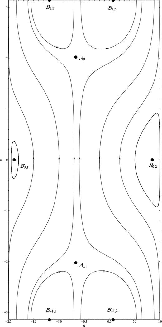
The results above indicate that the phase space has at most six fixed points, but our inability to solve equation (74) in the general case prevents us from giving a complete general analysis. Thus, here we limit ourselves to show, in Fig. 1, a sample of the phase space for a specific choice of the parameters, in order to give an idea of the kind of structures that one is likely to encounter in this analysis.

Figure 1.

$Sample of the phase space of the system (54) and (55). The line connecting the points $\mathcal {A}_0$ and $\mathcal {A}_1$ is an invariant submanifold. On this submanifold, $\mathcal {A}_0$ is an attractor.$

Open in new tab Download slide

Sample of the phase space of the system (54) and (55). The line connecting the points |$\mathcal {A}_0$| and |$\mathcal {A}_1$| is an invariant submanifold. On this submanifold, |$\mathcal {A}_0$| is an attractor.

5.5.2 Exact solution for H(t)

We now derive an analytical solution for the time variation of H. The availability of a closed-form solution for H(t) allows us to obtain immediately the time evolution of cos h_* via inversion of Hamiltonian (27).¹¹ With H(t) and cos h_*(t) it is then possible in principle to integrate the equations of motion for the remaining coordinates. Additionally, the analytical expression will allow us to calculate exactly the period of the oscillatory motion of H(t) and to make quantitative predictions about the behaviour of real physical systems in Section 6.

Recalling the form of Hamiltonian (27) and combining it with the equation for H,

\begin{equation} \frac{{\rm d}H}{{\rm d}t}=\epsilon \mathcal {F}_{1}\sin h_\ast , \end{equation}

(76)

we have

\begin{equation} \frac{{\rm d}H}{{\rm d}t}=\pm \sqrt{\epsilon ^{2}\mathcal {F}_{1}^{2}-\left(\mathcal {H}^{\prime }-\mathcal {H}_{N}-\epsilon \mathcal {F}_{0}\right)^{2}}, \end{equation}

(77)

where |$\mathcal {H}^\prime$| is the Hamiltonian constant (whose value is computed by substituting the initial values of the canonical variables in equation 27), and with the understanding that the plus sign is now to be taken when |$\epsilon \mathcal {F}_{1}$| and sin h_* have the same sign. At this point, it can be easily proven by direct calculations that the terms in H⁶ and H⁵ cancel out so that the radicand in equation (77) is a quartic polynomial in H. Following Whittaker & Watson (1927), we can then elect

\begin{eqnarray} f_{4}\left(H\right) &=& \epsilon ^{2}\mathcal {F}_{1}^{2}-\left(\mathcal {H}^{\prime }-\mathcal {H}_{N}-\epsilon \mathcal {F}_{0}\right)^{2}\nonumber \\ &=& a_{4}+4a_{3}H+6a_{2}H^{2}+4a_{1}H^{3}+a_{0}H^{4}, \end{eqnarray}

(78)

and rewrite equation (77) as

\begin{equation} \int _{H_{0}}^{H}\pm \frac{{\rm d}x}{\sqrt{f_{4}(x)}}=\int _{t_{0}}^{t}{\rm d}\tau , \end{equation}

(79)

where H₀ is the initial value of H and t₀ is the initial time. The coefficients of f₄(H) are reproduced in full form in Appendix C. The left-hand side of this equation is, apart from the sign ambiguity, an elliptic integral in standard form. A formula by Weierstrass (see Whittaker & Watson 1927, section 20.6) allows us to write the upper limit of the integral on the left-hand side as a function of the right-hand side. Specifically, if

\begin{equation} z=\int _{a}^{x}\left\lbrace f_{4}\left(t\right)\right\rbrace ^{-\frac{1}{2}}{\rm d}t, \end{equation}

(80)

where a is any constant, then

\begin{eqnarray} x\left(z\right) &=& a + \frac{1}{2\left[\wp \left(z\right)-\frac{1}{24}f_{4}^{\prime \prime }\left(a\right)\right]^{2} -\frac{1}{48}f_{4}\left(a\right)f_{4}^{iv}\left(a\right)}\nonumber \\ &&\times\left\lbrace \frac{1}{2}f_{4}^{\prime }\left(a\right)\left[\wp \left(z\right) -\frac{1}{24}f_{4}^{\prime \prime }\left(a\right)\right]+\frac{1}{24}f_{4}\left(a\right)f_{4}^{\prime \prime \prime }\left(a\right) \right.\nonumber \\ &&\ \ \left.+\ \sqrt{f_{4}\left(a\right)}\wp ^{\prime }\left(z\right) {\frac{1}{2}f_{4}^{\prime }\left(a\right)\left[\wp \left(z\right) -\frac{1}{24}f_{4}^{\prime \prime }\left(a\right)\right]} \right\rbrace , \end{eqnarray}

(81)

where ℘(z) ≡ ℘(z; g₂, g₃) is a Weierstrass elliptic function defined in terms of the invariants

\begin{equation} g_{2} = a_{0}a_{4}-4a_{1}a_{3}+3a_{2}^{2}, \end{equation}

(82)

\begin{equation} g_{3} = a_{0}a_{2}a_{4}+2a_{1}a_{2}a_{3}-a_{2}^{3}-a_{0}a_{3}^{2}-a_{1}^{2}a_{4}, \end{equation}

(83)

and the derivatives of f₄ are intended with respect to the polynomial variable. After the removal of the sign ambiguity in equation (79), detailed in Appendix D, the time evolution of H is thus given by

\begin{eqnarray} H\left(t\right) &=& H_{0}+\frac{1}{2\left[\wp \left(t\right)-\frac{1}{24}f_{4}^{\prime \prime }\left(H_{0}\right)\right]^{2}-\frac{1}{48}f_{4}\left(H_{0}\right)f_{4}^{iv}\left(H_{0}\right)}\nonumber \\ && \times\left\lbrace \frac{1}{2}f_{4}^{\prime }\left(H_{0}\right)\left[\wp \left(t\right) -\frac{1}{24}f_{4}^{\prime \prime }\left(H_{0}\right)\right] \right.\nonumber \\ &&\ \ +\ \left.\,\frac{1}{24}f_{4}\left(H_{0}\right)f_{4}^{\prime \prime \prime }\left(H_{0}\right) \pm \sqrt{f_{4}\left(H_{0}\right)}\wp ^{\prime }\left(t\right){ \frac{1}{2}f_{4}^{\prime }\left(H_{0}\right)\left[\wp \left(t\right) -\frac{1}{24}f_{4}^{\prime \prime }\left(H_{0}\right)\right] }\right\rbrace , \end{eqnarray}

(84)

where the ± sign is chosen based on the initial signs of sin h_* and |$\mathcal {F}_{1}$|⁠, and we set the initial time t₀ = 0 for convenience.

It is now useful to recall some basic properties of ℘(t) (Abramowitz & Stegun 1964). First of all, since in our case the invariants g₂ and g₃ are defined to be purely real and t is also limited to real values, ℘(t) and H(t) become real-valued periodic functions. The period of ℘(t), ℘^′(t) and H(t) is related to the invariants g₂ and g₃ via formulae involving elliptic integrals and the roots e₁, e₂ and e₃ of the cubic equation

\begin{equation} 4t^{3}-g_{2}t-g_{3}=0. \end{equation}

(85)

The sign of the modular discriminant

\begin{equation} \Delta =g_{2}^{3}-27g_{3}^{2} \end{equation}

(86)

determines the nature of the roots e₁, e₂ and e₃ of the cubic equation (85) and thus also the value of the period.

℘(t) can degenerate into a non-periodic function when Δ = 0. In particular, if g₂ = g₃ = 0, ℘(t) simply becomes

\begin{equation} \wp \left(t\right)=\frac{1}{t^{2}}. \end{equation}

(87)

If g₂ > 0 and g₃ < 0, the case Δ = 0 degenerates instead to

\begin{equation} \wp \left(t\right)=e_{1}+\frac{3e_{1}}{\left\lbrace \sinh \left[\left(3e_{1}\right)^{\frac{1}{2}}t\right]\right\rbrace ^{2}}, \end{equation}

(88)

where e₁ = e₂ > 0 and e₃ = −2e₁. For g₂ > 0 and g₃ > 0, the case Δ = 0 simplifies to

\begin{equation} \wp \left(t\right)=-\frac{e_{1}}{2}+\frac{\frac{3}{2}e_{1}}{\left\lbrace \sin \left[\left(\frac{3}{2}e_{1}\right)^{\frac{1}{2}}t\right]\right\rbrace ^{2}}, \end{equation}

(89)

where e₁ > 0 and e₂ = e₃ < 0. When ℘(t) is non-periodic, for t → ∞ H(t) tends to a finite value.

In addition to the degenerate cases of ℘(t), H(t) can degenerate also via particular values of H₀. For instance, if f₄(H₀) = f′₄(H₀) = 0, it is then clear from equation (84) that H(t) degenerates to

\begin{equation} H\left(t\right)=H_{0}, \end{equation}

(90)

which corresponds to an equilibrium point for H. It is straightforward, although tedious if done by hand, to check by substitution that the equilibrium condition found in equation (56), |$H_{0}=G^{2}/\mathcal {J}_{2}$|⁠, leads to the condition f₄(H₀) = f′₄(H₀) = 0. Another equilibrium condition that can be checked via substitution is the geometric configuration in which both the mean orbital angular momentum and the secondary body's mean spin are initially aligned to the spin of the primary, that is, H₀ = G and |$\tilde{H}_{\ast }=G+\tilde{G}$|⁠. This approach allows us to sidestep difficulties in verifying this equilibrium condition (which results in indeterminate forms due to |$G_{xy}=\tilde{G}_{xy\ast }=0$| and h_* being undefined) within the dynamical system framework.

As a special case of the general formula (84), we can analyse the behaviour of H(t) when J₂ = 0 (i.e. the particular case of geodetic precession examined in Section 5.4). It is easy to check by substitution (see formulae in Appendix C) that in this case the coefficients a₀ and a₁ of the quartic polynomial f₄(H) are both zero, and thus

\begin{eqnarray} g_{2} &=& 3a_{2}^{2}, \end{eqnarray}

(91)

\begin{eqnarray} g_{3} &=& -a_{2}^{3}, \end{eqnarray}

(92)

with

\begin{eqnarray} a_{2} &=& -\frac{1}{2}\epsilon \frac{m_{2}^{4}\mathcal {G}^{4}\mathcal {H}^{\prime }}{G^{3}L^{3}} +\frac{15}{16}\epsilon ^{2}\frac{m_{2}^{8}\mathcal {G}^{8}}{G^{3}L^{7}} +\frac{1}{4}\epsilon \frac{\tilde{G}^{2}m_{2}^{4}\mathcal {G}^{4}\mathcal {I}_{1}}{G^{3}L^{3}}\nonumber \\ &&-\frac{15}{8}\epsilon ^{2}\frac{m_{2}^{8}\mathcal {G}^{8}}{G^{4}L^{6}} -\frac{3}{8}\epsilon ^{2}\frac{\tilde{G}^{2}m_{2}^{8}\mathcal {G}^{8}}{G^{6}L^{6}} -\frac{1}{4}\epsilon \frac{m_{2}^{6}\mathcal {G}^{6}}{G^{3}L^{5}}, \end{eqnarray}

(93)

and the modular discriminant Δ is also null. As explained earlier and depending on the sign of g₃, in this configuration ℘(t) is either a simplified periodic function of the form (89) or a non-periodic function of the form (88). However, it is easy to check by substitution of |$\mathcal {H}^{\prime }$| that

\begin{eqnarray} a_{2} &=& -\frac{3}{8}\epsilon ^2\frac{m_2^8\mathcal {G}^8}{L^6G^6}\left[G^2-2H_0^2+2H_0\tilde{H}_\ast +\tilde{G}^2\right.\nonumber \\ &&{\frac{3}{8}\epsilon ^2\frac{m_2^8 {G}^8}{L^6G^6}}+\,\left.2G_{xy,0}\tilde{G}_{xy,0}\cos h_{\ast ,0}\right], \end{eqnarray}

(94)

where the zero subscript represents initial values. It is straightforward to verify how the quantity in the square brackets is the square of the magnitude M of the total mean angular momentum vector, and therefore it cannot be a negative quantity. As a first consequence, g₃ is always positive and the behaviour of H(t) is restricted to be purely periodic. Secondly, according to equation (89) and keeping in mind that e₁ = −a₂, the angular velocity of the periodic motion of H(t) is

\begin{equation} 2\sqrt{\frac{3}{2}e_1} = 2\sqrt{\frac{9}{16}\epsilon ^2\frac{m_2^8\mathcal {G}^8}{L^6G^6}M^2} = \frac{3}{2}\epsilon \frac{m_2^4\mathcal {G}^4}{L^3G^3}M \end{equation}

(95)

[the factor 2 arising from the fact that in equation (89) the sine is squared], which is in agreement with the precessional angular velocity (51) calculated for the geodetic effect.¹²

6 APPLICATION TO PHYSICAL SYSTEMS

We are now ready to apply the machinery we have developed so far to some real physical systems. We will consider three examples of interest: a Mercury-like planet, an exoplanet in a close orbit around a pulsar and the Earth-orbiting Gravity Probe B experiment. It is clear that because of our initial assumptions we will consider highly idealized systems; we have to stress again that our goal here is not to produce accurate predictions of the dynamical evolution of realistic physical models, but rather to highlight the role that relativistic effects play in the long term.

We will find that in all cases the spin–orbit and spin–spin couplings induce periodic oscillations of the mean orbital plane and, at the same time, of the mean spin vector. Such effects are typically small for the orbital plane, but, because of the conservation of the z-component of the total angular momentum |$\tilde{H}_\ast$|⁠, they correspond to non-negligible oscillations in the orientation of the mean spin.

We have to point out that the perturbative treatment outlined in the previous sections produces results in terms of the components of the mean angular momentum vectors with respect to a fixed (non-rotating) centre-of-mass reference system (rather than in terms of obliquity and relative orientations). Therefore, in the geometrical interpretations of our results, we will always be referring to absolute (as opposed to relative) orientation angles.

Given the small magnitude of the quantities involved in the computations, in order to avoid numerical issues we performed all calculations using the mpmath multiprecision library (Johansson et al. 2012).

6.1 Mercury-like planet

In the simplified case in which the Sun is a rigid homogeneous sphere rotating around a fixed axis, and a Mercury-like planet is the only body orbiting it, a set of possible initial values for the parameters of the system are displayed in Table 2. The parameters correspond to a Mercury-sized object orbiting at 0.47 au from the Sun in an orbit with eccentricity 0.2 and inclination 7°. The plane of the ecliptic is identified as being perpendicular to the spin axis of the Sun. The planet rotates with a period of 1405 h, and the absolute inclination of its spin vector is close to the value of the orbital inclination. Its radius r₁ is 2439 km.

Table 2.

Initial values (in SI units) for the parameters of a simplified Sun–Mercury two-body system.

Parameter	Value (SI units)
L₀	2.77 × 10¹⁵
G₀	2.71 × 10¹⁵
H₀	2.69 × 10¹⁵
\|$\tilde{G}_{0}$\|	2.95 × 10⁶
\|$\tilde{H}_{0}$\|	2.93 × 10⁶
J₂	1.12 × 10⁴²
r₁	6.37 × 10⁶

Open in new tab

Table 2.

Initial values (in SI units) for the parameters of a simplified Sun–Mercury two-body system.

Parameter	Value (SI units)
L₀	2.77 × 10¹⁵
G₀	2.71 × 10¹⁵
H₀	2.69 × 10¹⁵
\|$\tilde{G}_{0}$\|	2.95 × 10⁶
\|$\tilde{H}_{0}$\|	2.93 × 10⁶
J₂	1.12 × 10⁴²
r₁	6.37 × 10⁶

Open in new tab

Fig. 2 shows the time evolution of the absolute axial and orbital inclinations of the planet for different initial values of the angle h_*. The period of the evolution, calculated from the solution for H(t) in terms of elliptic functions, is 6.03 Ma. When h_{*, 0} = 0 the system is almost in equilibrium, as the initial axial and orbital inclinations are almost equal and almost parallel to the Sun's spin vector. The amplitude of the periodic oscillation increases together with h_{*, 0}. The oscillation is much wider in axial than in orbital inclination; this is a consequence of the fact that for this system |$G\gg \tilde{G}$|⁠: the conservation of |$\tilde{H}_{\ast }=H+\tilde{H}$|⁠, G and |$\tilde{G}$| imposes that a small change in the z-component of the mean orbital angular momentum, H, is proportionally a much larger change in the z-component of the mean spin vector, |$\tilde{H}$|⁠.

Figure 2.

Open in new tab Download slide

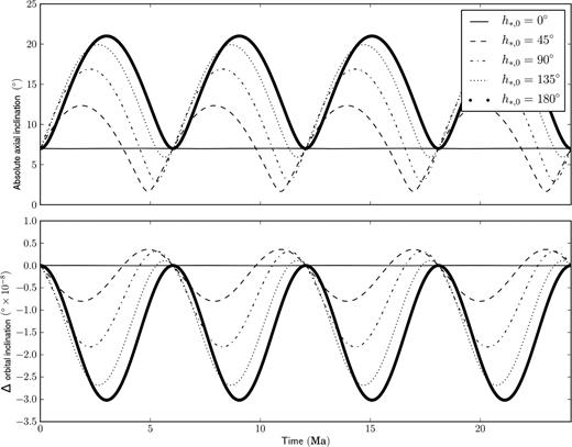
Time evolution of the absolute axial (top panel) and orbital (bottom panel) inclinations of a Mercury-like object orbiting the Sun. In the bottom panel, the quantity on the y-axis is the difference from the initial value of orbital inclination. The different curves correspond to different initial values for h_*. Time is measured in millions of years.

The main effect that can be observed in Fig. 2 is the geodetic precession. Indeed, in this dynamical system the slow rotations of both the planet and the Sun minimize the spin–spin interactions, and effectively relegate the spin–orbit effects to a precession of the planet's mean spin axis around the mean orbital angular momentum vector. This can be verified by noting that the precessional rate given by equation (51) yields essentially the same period of 6.03 Ma as the general formula in terms of elliptic functions.

The correlation between the oscillation amplitude and h_{*, 0} has a simple geometrical interpretation: when h_{*, 0} = 0, the mean spin and orbital angular momentum vectors share the same inclination (7°) and nodal angle, and therefore they are parallel (i.e. their relative angular separation is zero) and no precession motion takes place; as the difference in initial nodal angles (i.e. h_{*, 0}) increases, the relative angular separation between the two vectors increases too and the mean spin precesses around the mean orbital angular momentum vector. When h_{*, 0} = π, the initial angular separation reaches the maximum possible value, and the projection of the precession motion on the z-axis (which is what is visualized in Fig. 2) reaches its maximum oscillatory amplitude too.

6.2 Pulsar planet

In this second case, the central body is a millisecond pulsar with a Jupiter-like planet in close orbit. The parameters of the system are displayed in Table 3, and they are similar to the estimated parameters of the PSR J1719−1438 system (Bailes et al. 2011): the mass of the star is 1.4 M_⊙, its spin period is 5.8 ms and its diameter is 20 km, while the planet has a mass roughly equal to Jupiter (1.02M_J) and a radius of 0.4r_J, orbiting on a moderately inclined (i = 20°) near-circular (e = 0.06) orbit with semi-major axis of 600 000 km. Lacking estimates on the rotational state of the planet, we hypothesize a spin period similar to Jupiter (10 h) and an absolute inclination of the spin vector of 10°. As in the preceding case, the plane of the ecliptic is identified as being perpendicular to the spin axis of the star.

Table 3.

Initial values (in SI units) for the parameters of a pulsar–Jovian planet two-body system.

Parameter	Value (SI units)
L₀	3.33 × 10¹⁴
G₀	3.32 × 10¹⁴
H₀	3.12 × 10¹⁴
\|$\tilde{G}_{0}$\|	5.32 × 10¹⁰
\|$\tilde{H}_{0}$\|	5.23 × 10¹⁰
J₂	4.83 × 10⁴¹
r₁	2.76 × 10⁷

Open in new tab

Table 3.

Initial values (in SI units) for the parameters of a pulsar–Jovian planet two-body system.

Parameter	Value (SI units)
L₀	3.33 × 10¹⁴
G₀	3.32 × 10¹⁴
H₀	3.12 × 10¹⁴
\|$\tilde{G}_{0}$\|	5.32 × 10¹⁰
\|$\tilde{H}_{0}$\|	5.23 × 10¹⁰
J₂	4.83 × 10⁴¹
r₁	2.76 × 10⁷

Open in new tab

Fig. 3 shows the time evolution of the absolute axial and orbital inclinations of the planet for different initial values of the angle h_*. The period of the evolution is much shorter than in the previous case, amounting to circa 40 yr. This system is lacking an almost-equilibrium point for h_{*, 0} = 0, as the initial values of the inclinations are not close (although the amplitude of the oscillation is still correlated to h_{*, 0}). As in the previous case, the amplitude of the oscillation for the axial inclination dominates over the oscillation in orbital inclination, but since the |$\tilde{G}/G$| ratio is now larger the oscillation in orbital inclination is also larger, reaching almost 0| ${.\!\!\!\!\!\!^{\circ}}$|01 when h_{*, 0} = 180°.

Figure 3.

Open in new tab Download slide

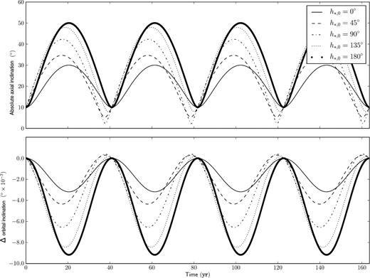
Time evolution of the absolute axial (top panel) and orbital (bottom panel) inclinations of a pulsar planetary two-body system. In the bottom panel, the quantity on the y-axis is the difference from the initial value of orbital inclination. Time is measured in years.

6.3 Earth-orbiting gyroscope

In this last example, we consider the gravitomagnetic effects on a gyroscope in low orbit on board a spacecraft around the Earth. The parameters of the system are taken from the experimental setup of the Gravity Probe B mission (Everitt et al. 2011): the orbit is polar (i = 90| ${.\!\!\!\!\!\!^{\circ}}$|007) with a semi-major axis of 7027 km and low eccentricity (e = 0.0014). The gyroscope consists of a rapidly rotating quartz sphere (38 mm diameter) whose spin axis is lying on the Earth's equatorial plane (i.e. the spin plane is also ‘polar’). The spin vector of the gyroscope and the orbital angular momentum vector of the spacecraft, both lying on the equatorial plane, are perpendicular to each other. Translated into mean Delaunay and SA parameters, this initial geometric configuration implies H ∼ 0, |$\tilde{H}_{\ast }\sim 0$|⁠, G_xy ∼ G, |$\tilde{G}_{xy\ast }\sim \tilde{G}$| and h_* = ±π/2 [with the sign depending on the values of h and |$\tilde{h}$| – note that in Everitt et al. (2011) the configuration shown in fig. 1 implies h_* = −π/2]. The substitution of these values in the general formula for H(t) yields a period of roughly 195 ka.

Now, turning our attention to the equations of motion, we first note that, given the time-scale of the time-evolution for H, we can consider H and h_* as constants for the duration of the Gravity Probe B experiment. With this assumption, the equation of motion for |$\tilde{h}$| radically simplifies to

\begin{equation} \frac{{\rm d}\tilde{h}}{{\rm d}t}=\frac{1}{2}\epsilon \frac{m_{2}^{3}\mathcal {G}^{4}J_{2}}{L^{3}G^{3}}, \end{equation}

(96)

and thus |$\tilde{h}$| evolves linearly with time. This is the expected frame-dragging precession, which, after substitution of the appropriate numerical values, amounts to circa 0.04 arcsec yr⁻¹ (Everitt et al. 2011). The effect corresponds to a movement of the mean spin axis of the gyroscope along the equatorial plane in the direction of the rotation of the Earth. The other expected relativistic motion is the geodetic effect, which is a drift of the mean spin axis on the orbital plane in the direction of the orbital motion. Translated into mean SA variables, this effect affects the element |$\tilde{H}=\tilde{H}_{\ast }-H$|⁠. Recalling that |$\tilde{H}_{\ast }$| is a constant of motion and that in our experimental setup H ∼ 0 and G_xy ∼ G, the time evolution of |$\tilde{H}$| is then given by

\begin{equation} \frac{{\rm d}\tilde{H}}{{\rm d}t}=-\frac{{\rm d}H}{{\rm d}t}=-\frac{3}{2}\epsilon \frac{\tilde{G}_{xy\ast }m_{2}^{4}\mathcal {G}^{4}}{L^{3}G^{2}}\sin h_{\ast }. \end{equation}

(97)

Recalling now that |$\tilde{H}=\tilde{G}\cos I$| by definition, where I is the inclination of the mean spin vector with respect to the z-axis and |$\tilde{G}$| is a constant of motion, we can write

\begin{equation} \frac{{\rm d}\tilde{H}}{{\rm d}t}=\tilde{G}\frac{{\rm d}\cos I}{{\rm d}t}, \end{equation}

(98)

and since |$\tilde{G}\sim \tilde{G}_{xy\ast }$| and I ∼ π/2, a Taylor expansion of cos I gives the simplified formula

\begin{equation} \frac{{\rm d}I}{{\rm d}t}=\frac{3}{2}\epsilon \frac{m_{2}^{4}\mathcal {G}^{4}}{L^{3}G^{2}}\sin h_{\ast }. \end{equation}

(99)

Depending then on the orientation of the angular momentum and spin vectors, h_* = ±π/2, and the time variation of I then becomes

\begin{equation} \frac{{\rm d}I}{{\rm d}t}=\pm \frac{3}{2}\epsilon \frac{m_{2}^{4}\mathcal {G}^{4}}{L^{3}G^{2}}. \end{equation}

(100)

Substitution of the numerical values in this formula yields the expected value of circa ±6.6 arcsec yr⁻¹.

7 CONCLUSIONS AND FUTURE WORK

In this paper, we have analysed the post-Newtonian evolution of the restricted relativistic two-body problem with spin. Our analysis has been performed via a modern perturbation scheme based on Lie series. The first important advantage of this method is that it allows us to work out all the calculations in a closed analytic form, thus permitting an analysis of long-term perturbative effects which are otherwise very difficult to detect with numerical techniques. Secondly, the Lie series formalism can be iterated to higher post-Newtonian orders using essentially the same procedure as employed in this study, and the connection between the transformed coordinates at each perturbative step is given by explicit formulae [contrary to the classical von Zeipel method (von Zeipel 1916)]. Finally, the Lie series methodology can be easily implemented on computer algebra systems, thus relegating the most cumbersome parts of the development of the theory to automatized algebraic manipulation.

Our analysis reproduces well-known classical results such as the relativistic pericentre precession, and the Lens–Thirring and geodetic effects. In addition, we are able to thoroughly investigate the complex interplay between spin and orbit, and we provide a novel solution for the full averaged equations of motion in terms of Weierstrass elliptic functions. This result is particularly interesting as it establishes a connection with recent developments in the exact solution of geodesic equations (see e.g. Hackmann et al. 2010; Scharf 2011; Gibbons & Vyska 2012), which also employ elliptic and hyperelliptic functions.

From the mathematical point of view, our investigation highlights the existence of a rich dynamical environment, with multiple sets of fixed points and aperiodic solutions arising with particular choices of initial conditions. From a physical point of view, we have shown how some of these exotic configurations appear in correspondence with initial conditions for which the approximation of our model starts to be unrealistic. In this sense, the generalization of these results to a full two-body model (to be tackled in an upcoming publication) will provide a more realistic insight into the physics of these particular solutions.

The application of our results to real physical systems shows how relativistic effects can accumulate over time to induce substantial changes in the dynamics. In particular, the absolute orientation of the spin vector of planetary-sized bodies in the Solar system undergoes significant changes, driven chiefly by the geodetic effect, over geological time-scales. In close pulsar planets, the evolution time shortens drastically to few years, and the effects on the planet's orbit increase by multiple orders of magnitude. In this sense, our results could be used to devise new tests of General Relativity based on precise measurements of the orbital parameters of pulsar planets and similar dynamical systems.

1

There are in truth other reasons why all our tests are focused on weak field: we live in a weak gravitational field and it is impossible to control gravitational fields like we do, for example, with electromagnetism.

2

To be precise, in the same period other researchers proposed alternative methods based on different assumptions (Fock 1964; Papapetrou 1974), but they all lead to the same results.

3

We were able to locate two papers in the existing literature that tackle the solution of the post-Newtonian equations using Lie series (Richardson & Kelly 1988; Heimberger, Soffel & Ruder 1990), none of them considering spin interactions.

4

The monopole–quadrupole interaction terms for compact bodies will depend on their internal structure and equations of state. For black holes, they are given, for example, in Damour (2001).

5

Vice versa, short-term periodic variations of the post-Newtonian elements will have amplitudes of order 1/c² and the precise connection with the Newtonian elements therefore becomes important.

6

This reference system is referred to as ‘invariable’ in Gurfil et al. (2007).

7

This transformation is reminiscent of the treatment of single-resonance dynamics in the N-body problem (see Lemma 4 in Morbidelli & Giorgilli 1993).

8

This is analogous to the coordinates in the Delaunay set becoming undefined for zero inclination/eccentricity.

9

The geometrical interpretation of the equilibrium points can be verified with the help of equations (25) and (26) and Table 1.

10

This is of course an expected result, since equilibrium points in 1 degree-of-freedom Hamiltonian systems must either be centres, saddles or have a double zero eigenvalue (Arnold 1989).

11

This, of course, is not possible if singular equilibrium points are present or if we are dealing with the indeterminate forms arising when the nodal angles are undefined.

12

In formula (51), the z-component of the total mean angular momentum |$\tilde{H}_\ast$| coincides with M in formula (95), as in equation (51) the total mean angular momentum is aligned to the z-axis.

REFERENCES

Abramowitz

M.

,

Stegun

I.

. ,

Handbook of Mathematical Functions, 5th edn

,

1964

New York

Dover

Google Scholar

Google Preview

OpenURL Placeholder Text

WorldCat

Arnold

V. I.

. ,

Mathematical Methods of Classical Mechanics, 2nd edn

,

1989

Berlin

Springer-Verlag

Google Scholar

Google Preview

OpenURL Placeholder Text

WorldCat

Bailes

M.

, et al. ,

Sci

,

2011

, vol.

333

pg.

1717

Crossref

Search ADS

Barker

B. M.

,

O'Connell

R. F.

. ,

Phys. Rev. D

,

1970

, vol.

2

pg.

1428

Crossref

Search ADS

Barker

B. M.

,

O'Connell

R. F.

. ,

Phys. Rev. D

,

1975

, vol.

12

pg.

329

Crossref

Search ADS

Barker

B. M.

,

O'Connell

R. F.

. ,

Phys. Rev. D

,

1976

, vol.

14

pg.

861

Crossref

Search ADS

Barker

B. M.

,

O'Connell

R. F.

. ,

Gen. Relativ. Gravit.

,

1979

, vol.

11

pg.

149

Crossref

Search ADS

Biscani

F.

. ,

PhD dissertation

,

2008

Univ. Padua

Bogorodskii

A. F.

. ,

Sov. Astron.

,

1959

, vol.

3

pg.

857

Brumberg

V.

. ,

Essential Relativistic Celestial Mechanics

,

1991

New York

Taylor & Francis

Google Scholar

Google Preview

OpenURL Placeholder Text

WorldCat

Cugusi

L.

,

Proverbio

E.

. ,

A&A

,

1978

, vol.

69

pg.

321

Damour

T.

. ,

Phys. Rev. D

,

2001

, vol.

64

pg.

124013

Crossref

Search ADS

Damour

T.

,

Soffel

M.

,

Xu

C.

. ,

Phys. Rev. D (Particles and Fields)

,

1991a

, vol.

43

pg.

3273

Crossref

Search ADS

Damour

T. M. A. G.

,

Soffel

M. H.

,

Xu

C.

. ,

Phys. Rev. D

,

1991b

, vol.

45

pg.

1017

Crossref

Search ADS

Damour

T.

,

Soffel

M.

,

Xu

C.

. ,

Phys. Rev. D (Particles and Fields)

,

1993

, vol.

47

pg.

3124

Crossref

Search ADS

Damour

T.

,

Soffel

M.

,

Xu

C.

. ,

Phys. Rev. D (Particles and Fields)

,

1994

, vol.

49

pg.

618

Crossref

Search ADS

Damour

T.

,

Jaranowski

P.

,

Schäfer

G.

. ,

Phys. Rev. D

,

2008

, vol.

78

pg.

024009

Crossref

Search ADS

de Sitter

W.

. ,

MNRAS

,

1916

, vol.

77

pg.

155

Crossref

Search ADS

Deprit

A.

. ,

Celest. Mech.

,

1969

, vol.

1

pg.

12

Crossref

Search ADS

Deprit

A.

. ,

Celest. Mech.

,

1982

, vol.

26

pg.

9

Crossref

Search ADS

Einstein

A.

. ,

Ann. Phys., Lpz.

,

1916

, vol.

354

pg.

769

Crossref

Search ADS

Einstein

A.

,

Infeld

L.

,

Hoffmann

B.

. ,

Ann. Math.

,

1938

, vol.

39

pg.

65

Crossref

Search ADS

Everitt

C.

, et al. ,

Phys. Rev. Lett.

,

2011

, vol.

106, 221101

Fock

V. A.

. ,

The Theory of Space, Time, and Gravitation, 2nd revised edn

,

1964

New York

MacMillan

(translated from a Russian publication by N. Kemmer)

Google Scholar

Google Preview

OpenURL Placeholder Text

WorldCat

Gibbons

G. W.

,

Vyska

M.

. ,

Class. Quantum Gravity

,

2012

, vol.

29

pg.

065016

Crossref

Search ADS

Gurfil

P.

,

Elipe

A.

,

Tangren

W.

,

Efroimsky

M.

. ,

Regular Chaotic Dyn.

,

2007

, vol.

12

pg.

389

Crossref

Search ADS

Hackmann

E.

,

Lämmerzahl

C.

,

Kagramanova

V.

,

Kunz

J.

. ,

Phys. Rev. D

,

2010

, vol.

81

pg.

044020

Crossref

Search ADS

Hees

A.

,

Wolf

P.

,

Lamine

B.

,

Jaekel

M. T.

,

Poncin-Lafitte

C. L.

,

Lainey

V.

,

Dehant

V.

. ,

2011

Testing Gravitation in the Solar System with Radio Science experiments, A&A (SF2A)

Heimberger

J.

,

Soffel

M.

,

Ruder

H.

. ,

Celest. Mech. Dyn. Astron.

,

1990

, vol.

47

pg.

205

Crossref

Search ADS

Hori

G.

. ,

PASJ

,

1966

, vol.

18

pg.

287

Johansson

F.

, et al. ,

2012

mpmath: a Python library for arbitrary-precision floating-point arithmetic (version 0.17)http://code.google.com/p/mpmath/

Kopeikin

S.

,

Efroimsky

M.

,

Kaplan

G.

. ,

Relativistic Celestial Mechanics of the Solar System

,

2011

Berlin

Wiley-VCH

Google Scholar

Google Preview

OpenURL Placeholder Text

WorldCat

Landau

L. D.

,

Lifschitz

E. M.

. ,

Course of Theoretical Physics – Pergamon International Library of Science, Technology, Engineering and Social Studies, 4th Revised English edn

,

1975

Oxford

Pergamon Press

Google Scholar

Google Preview

OpenURL Placeholder Text

WorldCat

Morbidelli

A.

. ,

Modern Celestial Mechanics: Aspects of Solar System Dynamics, 1st edn

,

2002

London

Taylor & Francis

Google Scholar

Google Preview

OpenURL Placeholder Text

WorldCat

Morbidelli

A.

,

Giorgilli

A.

. ,

Celest. Mech. Dyn. Astron.

,

1993

, vol.

55

pg.

131

Crossref

Search ADS

Murray

C. D.

,

Dermott

S. F.

. ,

Solar System Dynamics

,

2000

Cambridge

Cambridge Univ. Press

Google Scholar

Google Preview

OpenURL Placeholder Text

WorldCat

Palacián

J.

. ,

Chaos Solitons Fractals

,

2002

, vol.

13, 853

Papapetrou

A.

. ,

Lectures on General Relativity

,

1974

Dordrecht

Reidel

Google Scholar

Google Preview

OpenURL Placeholder Text

WorldCat

Peebles

P.

. ,

Principles of Physical Cosmology

,

1993

Princeton, NJ

Princeton Univ. Press

Google Scholar

Google Preview

OpenURL Placeholder Text

WorldCat

Richardson

D. L.

,

Kelly

T. J.

. ,

Celest. Mech.

,

1988

, vol.

43

pg.

193

Crossref

Search ADS

Scharf

G.

. ,

Journal of Modern Physics

,

2011

, vol.

2

pg.

274

Crossref

Search ADS

Schiff

L. I.

. ,

Proc. Natl. Acad. Sci. USA

,

1960a

, vol.

46

pg.

871

Crossref

Search ADS

Schiff

L. I.

. ,

Am. J. Phys.

,

1960b

, vol.

28

pg.

340

Crossref

Search ADS

Straumann

N.

. ,

General Relativity and Relativistic Astrophysics

,

1984

Berlin

Springer-Verlag

Google Scholar

Google Preview

OpenURL Placeholder Text

WorldCat

Thirring

H.

. ,

Phys. Z.

,

1918

, vol.

19

pg.

33

von Zeipel

H.

. ,

Ark. Mat, Astron. & Fys.

,

1916

, vol.

11, 1

Wex

N.

. ,

Class. Quantum Gravity

,

1995

, vol.

12

pg.

983

Crossref

Search ADS

Whittaker

E. T.

,

Watson

G. N.

. ,

A Course of Modern Analysis, 4th edn

,

1927

Cambridge

Cambridge Univ. Press

Google Scholar

Google Preview

OpenURL Placeholder Text

WorldCat

Wu

X.

,

Xie

Y.

. ,

Phys. Rev. D

,

2010

, vol.

81

pg.

084045

Crossref

Search ADS

APPENDIX A: CLOSED-FORM AVERAGING

We detail in this appendix the solution of equation (23), here reproduced for convenience:

\begin{equation} \chi =\int \frac{L^{3}}{\mathcal {G}^{2}m_{2}^{2}}\left(\mathcal {H}_{1}-\mathcal {K}\right){\rm d}l. \end{equation}

(A1)

From equation (14), the structure of |$\mathcal {H}_{1}$| is as follows:

\begin{eqnarray} \mathcal {H}_{1} &=& \mathcal {A}_{0}+\frac{\mathcal {A}_{1}}{r}+\frac{\mathcal {A}_{2}}{r^{2}}+\frac{1}{r^{3}}\left[\mathcal {A}_{3a}+\mathcal {A}_{3b}\cos \left(\tilde{h}-h\right)\right]\nonumber \\ && +\,\frac{1}{r^{3}}\left[\mathcal {B}_{0}\cos \left(2f+2g\right)+\mathcal {B}_{1}\cos \left(2f+2g+\tilde{h}-h\right)\right.\nonumber \\ && +\left.\mathcal {B}_{2}\cos \left(2f+2g-\tilde{h}+h\right)\right], \end{eqnarray}

(A2)

where the coefficients |$\mathcal {A}_{i}$| and |$\mathcal {B}_{i}$| are functions of the momenta only. As previously remarked, in this expression we have to consider r and f as implicit functions of L, G and l. For the solution of equation (A1), it is convenient to look for a |$\mathcal {K}$| in the form

\begin{equation} \mathcal {K}=\mathcal {A}_{0}+\mathcal {K}_{1}, \end{equation}

(A3)

where |$\mathcal {A}_{0}$| is a function of the momenta only from equation (A2). equation (A1) thus becomes

\begin{eqnarray} \chi &=& \frac{L^{3}}{\mathcal {G}^{2}m_{2}^{2}}\left[\int \left(\mathcal {H}_{1}-\mathcal {A}_{0}\right){\rm d}l-\int \mathcal {K}_{1}{\rm d}l\right]. \end{eqnarray}

(A4)

We use now the differential relation (Murray & Dermott 2000)

\begin{equation} {\rm d}l=\frac{r^{2}}{a^{2}\sqrt{1-e^{2}}}{\rm d}f=\frac{r^{2}\mathcal {G}^{2}m_{2}^{2}}{GL^{3}}{\rm d}f \end{equation}

(A5)

to change the integration variable in the first integral of equation (A4) from l to f:

\begin{equation} \chi =\frac{1}{G}\int r^{2}\left(\mathcal {H}_{1}-\mathcal {A}_{0}\right){\rm d}f-\frac{L^{3}}{\mathcal {G}^{2}m_{2}^{2}}\int \mathcal {K}_{1}{\rm d}l, \end{equation}

(A6)

where the first integrand in equation (A6) has now become

\begin{eqnarray} r^{2}\left(\mathcal {H}_{1}-\mathcal {A}_{0}\right) &=& r\mathcal {A}_{1}+\mathcal {A}_{2}+\frac{1}{r}\left[\mathcal {A}_{3a}+\mathcal {A}_{3b}\cos \left(\tilde{h}-h\right)\right]\nonumber \\ && +\,\frac{1}{r}\left[\mathcal {B}_{0}\cos \left(2f+2g\right) {\mathcal {B}_{1}\cos \left(2f+2g+\tilde{h}-h\right)} \right.\nonumber \\ && +\,\mathcal {B}_{1}\cos \left(2f+2g+\tilde{h}-h\right)\nonumber \\ && +\left.\mathcal {B}_{2}\cos \left(2f+2g-\tilde{h}+h\right)\right], \end{eqnarray}

(A7)

and the coefficients |$\mathcal {A}_{i}$| and |$\mathcal {B}_{i}$| are still functions of the momenta only. We now perform a further split of the first integrand in equation (A6), separating the term |$\mathcal {A}_1$| in its own integral:

\begin{eqnarray} \chi &=& \frac{1}{G}\int r\mathcal {A}_{1} {\rm d}f + \frac{1}{G} \int \left\lbrace \mathcal {A}_{2}+\frac{1}{r}\left[\mathcal {A}_{3a}+\mathcal {A}_{3b}\cos \left(\tilde{h}-h\right)\right]\right.\nonumber \\ && +\,\frac{1}{r}\left[\mathcal {B}_{0}\cos \left(2f+2g\right)+\mathcal {B}_{1}\cos \left(2f+2g+\tilde{h}-h\right)\right.\nonumber \\ && +\left. {\mathcal {A}_{2}+\frac{1}{r}\left[\mathcal {A}_{3a}+\mathcal {A}_{3b}\cos \left(\tilde{h}-h\right)\right]} \left. \mathcal {B}_{2}\cos \left(2f+2g-\tilde{h}+h\right)\right]\right\rbrace {\rm d}f -\frac{L^{3}}{\mathcal {G}^{2}m_{2}^{2}}\int \mathcal {K}_{1}{\rm d}l. \end{eqnarray}

(A8)

The next step is to change the integration variable in the first integrand of equation (A8) from the true anomaly f to the eccentric anomaly E via the standard differential relation

\begin{equation} {\rm d}f=\frac{a}{r}\sqrt{1-e^{2}}{\rm d}E=\frac{LG}{r\mathcal {G}m_{2}}{\rm d}E, \end{equation}

(A9)

where the eccentricity e is to be considered an implicit function of L and G and the eccentric anomaly E an implicit function of L, G and l. equation (A8) now reads

\begin{eqnarray} \chi &=& \frac{1}{G}\int\! \frac{\mathcal {A}_{1}LG}{\mathcal {G}m_{2}} {\rm d}E + \frac{1}{G} \int\! \left\lbrace \mathcal {A}_{2}+\frac{1}{r}\left[\mathcal {A}_{3a}+\mathcal {A}_{3b}\cos \left(\tilde{h}-h\right)\right]\right.\nonumber \\ && +\,\frac{1}{r}\left[\mathcal {B}_{0}\cos \left(2f+2g\right)+\mathcal {B}_{1}\cos \left(2f+2g+\tilde{h}-h\right)\right.\nonumber \\ && +\left. {\mathcal {A}_{2}+\frac{1}{r}\left[\mathcal {A}_{3a}+\mathcal {A}_{3b}\cos \left(\tilde{h}-h\right)\right]} \left. \mathcal {B}_{2}\cos \left(2f+2g-\tilde{h}+h\right)\right]\right\rbrace {\rm d}f -\frac{L^{3}}{\mathcal {G}^{2}m_{2}^{2}}\int \mathcal {K}_{1}{\rm d}l.\nonumber \\ \end{eqnarray}

(A10)

By substituting the standard relation

\begin{equation} \frac{1}{r} = \frac{1+e\cos f}{a\left(1-e^{2}\right)}=\frac{\mathcal {G}m_{2}}{G^{2}}+\frac{\mathcal {G}m_{2}}{G^{2}}e\cos f, \end{equation}

(A11)

in the second integrand of equation (A10), and after straightforward algebraic passages, equation (A10) becomes

\begin{eqnarray} \chi &=& \frac{1}{G}\left\lbrace \int \mathcal {C}_{1}{\rm d}E+\int \left[\mathcal {C}_{2,0}+\mathcal {C}_{2,1}\cos \left(\tilde{h}-h\right)\right]{\rm d}f{\int \sum _{j\ne 0,k,n,m}\mathcal {D}_{j,k,n,m}\left(jf+kg+n\tilde{h}+mh\right)df}\right.\nonumber \\ && +\left.\int \sum _{j\ne 0,k,n,m}\mathcal {D}_{jknm}\cos \left(jf+kg+n\tilde{h}+mh\right){\rm d}f\right\rbrace \nonumber \\ &&-\,\frac{L^{3}}{\mathcal {G}^{2}m_{2}^{2}}\int \mathcal {K}_{1}{\rm d}l, \end{eqnarray}

(A12)

where the |$\mathcal {C}$| and |$\mathcal {D}$| coefficients are functions of the momenta only, and the true anomaly f always appears in the cosines associated with the |$\mathcal {D}$| coefficients. We can now choose |$\mathcal {K}_{1}$| as

\begin{equation} \mathcal {K}_{1}=\frac{\mathcal {G}^{2}m_{2}^{2}}{GL^{3}}\left[\mathcal {C}_{1}+\mathcal {C}_{2,0}+\mathcal {C}_{2,1}\cos \left(\tilde{h}-h\right)\right], \end{equation}

(A13)

so that the final expression for the generator χ becomes

\begin{eqnarray} \chi &=& \frac{1}{G}\left\lbrace \mathcal {C}_{1}\left(E-l\right)+\left[\mathcal {C}_{2,0} +\mathcal {C}_{2,1}\cos \left(\tilde{h}-h\right)\right]\left(f-l\right) {\frac{1}{G}\int \sum _{j\ne 0,k,n,m}\mathcal {D}_{jknm}\cos \left(jf+kg+n\tilde{h}+mh\right)df} \right.\nonumber \\ &&+\left.\int \sum _{j\ne 0,k,n,m}\mathcal {D}_{jknm}\cos \left(jf+kg+n\tilde{h}+mh\right){\rm d}f\right\rbrace , \end{eqnarray}

(A14)

where the integral in this expression is trivially calculated (as the |$\mathcal {D}$| coefficients do not depend on f). χ has thus been defined as a 2π-periodic function in the angular coordinates. By plugging equation (A13) into equation (A3), we can now see how

\begin{equation} \mathcal {K}=\mathcal {E}_{0}+\mathcal {E}_{1}\cos \left(\tilde{h}-h\right), \end{equation}

(A15)

where the |$\mathcal {E}$| coefficients are functions of the momenta only. Finally, via this definition of |$\mathcal {K}$| and equations (21) and (20), we obtain equation (24):

\begin{equation} \mathcal {H}^{\prime }=\mathcal {H}_{\rm N}+\epsilon \left[\mathcal {E}_{0}+\mathcal {E}_{1}\cos \left(\tilde{h}-h\right)\right]. \end{equation}

(A16)

APPENDIX B: PARTIAL DERIVATIVES OF |$\mathcal {F}_0$| AND |$\mathcal {F}_1$|

The full form of the partial derivatives of |$\mathcal {F}_0$| with respect to the mean momenta appearing in equations (32) is

\begin{eqnarray} \frac{\mathrm{\partial} \mathcal {F}_0}{\mathrm{\partial} L} &=& -\,\frac{3}{2}\frac{{J_2}{\mathcal {G}}^{4}{\tilde{H}_\ast }{m_2}^{3}}{{G}^{3}{L}^{4}} -\frac{15}{2}\frac{{\mathcal {G}}^{4}{m_2}^{4}}{{L}^{5}} -\frac{9}{2}\frac{{H}{\mathcal {G}}^{4}{\tilde{H}_\ast }{m_2}^{4}}{{G}^{3}{L}^{4}}\nonumber \\ &&+\,\frac{9}{2}\frac{{H}^{2}{\mathcal {G}}^{4}{m_2}^{4}}{{G}^{3}{L}^{4}} -\frac{9}{2}\frac{{H}^{3}{J_2}{\mathcal {G}}^{4}{m_2}^{3}}{{G}^{5}{L}^{4}} +\frac{9}{2}\frac{{H}^{2}{J_2}{\mathcal {G}}^{4}{\tilde{H}_\ast }{m_2}^{3}}{{G}^{5}{L}^{4}}\nonumber \\ &&+\,9\frac{{\mathcal {G}}^{4}{m_2}^{4}}{{G}{L}^{4}}-\frac{9}{2}\frac{{H}{J_2}{\mathcal {G}}^{4}{m_2}^{3}}{{G}^{3}{L}^{4}}, \end{eqnarray}

(B1)

\begin{eqnarray} \frac{\mathrm{\partial} \mathcal {F}_0}{\mathrm{\partial} G} &=& -\,\frac{9}{2}\frac{{H}{J_2}{\mathcal {G}}^{4}{m_2}^{3}}{{G}^{4}{L}^{3}} +\frac{9}{2}\frac{{H}^{2}{\mathcal {G}}^{4}{m_2}^{4}}{{G}^{4}{L}^{3}} +\frac{15}{2}\frac{{H}^{2}{J_2}{\mathcal {G}}^{4}{\tilde{H}_\ast }{m_2}^{3}}{{G}^{6}{L}^{3}}\nonumber \\ && +\,3\frac{{\mathcal {G}}^{4}{m_2}^{4}}{{G}^{2}{L}^{3}} -\frac{3}{2}\frac{{J_2}{\mathcal {G}}^{4}{\tilde{H}_\ast }{m_2}^{3}}{{G}^{4}{L}^{3}} -\frac{15}{2}\frac{{H}^{3}{J_2}{\mathcal {G}}^{4}{m_2}^{3}}{{G}^{6}{L}^{3}}\nonumber \\ && -\,\frac{9}{2}\frac{{H}{\mathcal {G}}^{4}{\tilde{H}_\ast }{m_2}^{4}}{{G}^{4}{L}^{3}}, \end{eqnarray}

(B2)

\begin{eqnarray} \frac{\mathrm{\partial} \mathcal {F}_0}{\mathrm{\partial} H} &=& \frac{3}{2}\frac{{J_2}{\mathcal {G}}^{4}{m_2}^{3}}{{G}^{3}{L}^{3}} -3\frac{{H}{J_2}{\mathcal {G}}^{4}{\tilde{H}_\ast }{m_2}^{3}}{{G}^{5}{L}^{3}} +\frac{9}{2}\frac{{H}^{2}{J_2}{\mathcal {G}}^{4}{m_2}^{3}}{{G}^{5}{L}^{3}}\nonumber \\ && -\,3\frac{{H}{\mathcal {G}}^{4}{m_2}^{4}}{{G}^{3}{L}^{3}}+\frac{3}{2}\frac{{\mathcal {G}}^{4}{\tilde{H}_\ast }{m_2}^{4}}{{G}^{3}{L}^{3}}, \end{eqnarray}

(B3)

\begin{equation} \frac{\mathrm{\partial} \mathcal {F}_0}{\mathrm{\partial} \tilde{H}_\ast } = \frac{1}{2}\frac{{J_2}{\mathcal {G}}^{4}{m_2}^{3}}{{G}^{3}{L}^{3}}+\frac{3}{2}\frac{{H}{\mathcal {G}}^{4}{m_2}^{4}}{{G}^{3}{L}^{3}}-\frac{3}{2}\frac{{H}^{2}{J_2}{\mathcal {G}}^{4}{m_2}^{3}}{{G}^{5}{L}^{3}}. \end{equation}

(B4)

The partial derivatives of |$\mathcal {F}_1$| are instead

\begin{equation} \frac{\mathrm{\partial} \mathcal {F}_1}{\mathrm{\partial} L} = -\frac{9}{2}\frac{{G_{xy}}{\mathcal {G}}^{4}{\tilde{G}_{xy\ast }}{m_2}^{4}}{{G}^{3}{L}^{4}}+\frac{9}{2}\frac{{G_{xy}}{H}{J_2}{\mathcal {G}}^{4}{\tilde{G}_{xy\ast }}{m_2}^{3}}{{G}^{5}{L}^{4}}, \end{equation}

(B5)

\begin{eqnarray} \frac{\mathrm{\partial} \mathcal {F}_1}{\mathrm{\partial} G} &=& \frac{15}{2}\frac{{G_{xy}}{H}{J_2}{\mathcal {G}}^{4}{\tilde{G}_{xy\ast }}{m_2}^{3}}{{G}^{6}{L}^{3}} -\frac{9}{2}\frac{{G_{xy}}{\mathcal {G}}^{4}{\tilde{G}_{xy\ast }}{m_2}^{4}}{{G}^{4}{L}^{3}}\nonumber \\ &&+\,\frac{3}{2}\frac{{\mathcal {G}}^{4}{\tilde{G}_{xy\ast }}{m_2}^{4}}{{G}^{2}{G_{xy}}{L}^{3}} -\frac{3}{2}\frac{{H}{J_2}{\mathcal {G}}^{4}{\tilde{G}_{xy\ast }}{m_2}^{3}}{{G}^{4}{G_{xy}}{L}^{3}}, \end{eqnarray}

(B6)

\begin{eqnarray} \frac{\mathrm{\partial} \mathcal {F}_1}{\mathrm{\partial} H} &=& \frac{3}{2}\frac{{G_{xy}}{H}^{2}{J_2}{\mathcal {G}}^{4}{m_2}^{3}}{{G}^{5}{L}^{3}{\tilde{G}_{xy\ast }}} +\frac{3}{2}\frac{{H}^{2}{J_2}{\mathcal {G}}^{4}{\tilde{G}_{xy\ast }}{m_2}^{3}}{{G}^{5}{G_{xy}}{L}^{3}}\nonumber \\ &&+\frac{3}{2}\frac{{G_{xy}}{\mathcal {G}}^{4}{\tilde{H}_\ast }{m_2}^{4}}{{G}^{3}{L}^{3}{\tilde{G}_{xy\ast }}} -\frac{3}{2}\frac{{G_{xy}}{J_2}{\mathcal {G}}^{4}{\tilde{G}_{xy\ast }}{m_2}^{3}}{{G}^{5}{L}^{3}}\nonumber \\ &&-\frac{3}{2}\frac{{G_{xy}}{H}{\mathcal {G}}^{4}{m_2}^{4}}{{G}^{3}{L}^{3}{\tilde{G}_{xy\ast }}} -\frac{3}{2}\frac{{H}{\mathcal {G}}^{4}{\tilde{G}_{xy\ast }}{m_2}^{4}}{{G}^{3}{G_{xy}}{L}^{3}}\nonumber \\ &&-\frac{3}{2}\frac{{G_{xy}}{H}{J_2}{\mathcal {G}}^{4}{\tilde{H}_\ast }{m_2}^{3}}{{G}^{5}{L}^{3}{\tilde{G}_{xy\ast }}}, \end{eqnarray}

(B7)

\begin{eqnarray} \frac{\mathrm{\partial} \mathcal {F}_1}{\mathrm{\partial} \tilde{G}} &=& \frac{3}{2}\frac{{G_{xy}}{\mathcal {G}}^{4}{\tilde{G}}{m_2}^{4}}{{G}^{3}{L}^{3}{\tilde{G}_{xy\ast }}}-\frac{3}{2}\frac{{G_{xy}}{H}{J_2}{\mathcal {G}}^{4}{\tilde{G}}{m_2}^{3}}{{G}^{5}{L}^{3}{\tilde{G}_{xy\ast }}}, \end{eqnarray}

(B8)

\begin{eqnarray} \frac{\mathrm{\partial} \mathcal {F}_1}{\mathrm{\partial} \tilde{H}_\ast } &=& -\frac{3}{2}\frac{{G_{xy}}{\mathcal {G}}^{4}{\tilde{H}_\ast }{m_2}^{4}}{{G}^{3}{L}^{3}{\tilde{G}_{xy\ast }}} -\frac{3}{2}\frac{{G_{xy}}{H}^{2}{J_2}{\mathcal {G}}^{4}{m_2}^{3}}{{G}^{5}{L}^{3}{\tilde{G}_{xy\ast }}}\nonumber \\ &&+\frac{3}{2}\frac{{G_{xy}}{H}{\mathcal {G}}^{4}{m_2}^{4}}{{G}^{3}{L}^{3}{\tilde{G}_{xy\ast }}} +\frac{3}{2}\frac{{G_{xy}}{H}{J_2}{\mathcal {G}}^{4}{\tilde{H}_\ast }{m_2}^{3}}{{G}^{5}{L}^{3}{\tilde{G}_{xy\ast }}}. \end{eqnarray}

(B9)

APPENDIX C: COEFFICIENTS OF THE QUARTIC POLYNOMIAL

Here follows the full form of the coefficients of the polynomial f₄(H) in equation (78):

\begin{eqnarray} a_0 &=& -\frac{9}{4}\frac{{J_2}^{2}{\mathcal {G}}^{8}{\tilde{G}}^{2}{\epsilon }^{2}{m_2}^{6}}{{G}^{10}{L}^{6}} -\frac{27}{4}\frac{{J_2}^{2}{\mathcal {G}}^{8}{\epsilon }^{2}{m_2}^{6}}{{G}^{8}{L}^{6}}, \end{eqnarray}

(C1)

\begin{eqnarray} a_1 &=& \frac{9}{8}\frac{{J_2}{\mathcal {G}}^{8}{\tilde{G}}^{2}{\epsilon }^{2}{m_2}^{7}}{{G}^{8}{L}^{6}} +\frac{15}{8}\frac{{J_2}^{2}{\mathcal {G}}^{8}{\tilde{H}_\ast }{\epsilon }^{2}{m_2}^{6}}{{G}^{8}{L}^{6}} -\frac{45}{32}\frac{{J_2}{\mathcal {G}}^{8}{\epsilon }^{2}{m_2}^{7}}{{G}^{5}{L}^{7}}\nonumber \\ &&+\frac{9}{2}\frac{{J_2}{\mathcal {G}}^{8}{\epsilon }^{2}{m_2}^{7}}{{G}^{6}{L}^{6}} -\frac{3}{8}\frac{{J_2}{\mathcal {G}}^{4}{\mathcal {I}_1}{\tilde{G}}^{2}{\epsilon }{m_2}^{3}}{{G}^{5}{L}^{3}} +\frac{3}{8}\frac{{J_2}{\mathcal {G}}^{6}{\epsilon }{m_2}^{5}}{{G}^{5}{L}^{5}}\nonumber \\ &&+\frac{3}{4}\frac{{J_2}{\mathcal {G}}^{4}{\mathcal {H}^\prime }{\epsilon }{m_2}^{3}}{{G}^{5}{L}^{3}}, \end{eqnarray}

(C2)

\begin{eqnarray} a_2 &=& \frac{1}{4}\frac{{\mathcal {G}}^{4}{\mathcal {I}_1}{\tilde{G}}^{2}{\epsilon }{m_2}^{4}}{{G}^{3}{L}^{3}} -\frac{3}{8}\frac{{J_2}^{2}{\mathcal {G}}^{8}{\epsilon }^{2}{m_2}^{6}}{{G}^{6}{L}^{6}} -\frac{1}{8}\frac{{J_2}^{2}{\mathcal {G}}^{8}{\tilde{H}_\ast }^{2}{\epsilon }^{2}{m_2}^{6}}{{G}^{8}{L}^{6}}\nonumber \\ &&+\frac{15}{16}\frac{{\mathcal {G}}^{8}{\epsilon }^{2}{m_2}^{8}}{{G}^{3}{L}^{7}} -\frac{1}{2}\frac{{\mathcal {G}}^{4}{\mathcal {H}^\prime }{\epsilon }{m_2}^{4}}{{G}^{3}{L}^{3}} -\frac{1}{4}\frac{{\mathcal {G}}^{6}{\epsilon }{m_2}^{6}}{{G}^{3}{L}^{5}}\nonumber \\ &&+\frac{15}{16}\frac{{J_2}{\mathcal {G}}^{8}{\tilde{H}_\ast }{\epsilon }^{2}{m_2}^{7}}{{G}^{5}{L}^{7}} +\frac{3}{8}\frac{{J_2}^{2}{\mathcal {G}}^{8}{\tilde{G}}^{2}{\epsilon }^{2}{m_2}^{6}}{{G}^{8}{L}^{6}} -\frac{3}{8}\frac{{\mathcal {G}}^{8}{\tilde{G}}^{2}{\epsilon }^{2}{m_2}^{8}}{{G}^{6}{L}^{6}}\nonumber \\ &&-\frac{15}{8}\frac{{\mathcal {G}}^{8}{\epsilon }^{2}{m_2}^{8}}{{G}^{4}{L}^{6}} +\frac{1}{4}\frac{{J_2}{\mathcal {G}}^{4}{\mathcal {I}_1}{\tilde{G}}^{2}{\tilde{H}_\ast }{\epsilon }{m_2}^{3}}{{G}^{5}{L}^{3}}\nonumber \\ &&-\frac{1}{2}\frac{{J_2}{\mathcal {G}}^{4}{\mathcal {H}^\prime }{\tilde{H}_\ast }{\epsilon }{m_2}^{3}}{{G}^{5}{L}^{3}} -\frac{1}{4}\frac{{J_2}{\mathcal {G}}^{6}{\tilde{H}_\ast }{\epsilon }{m_2}^{5}}{{G}^{5}{L}^{5}}\nonumber \\ &&-\frac{7}{2}\frac{{J_2}{\mathcal {G}}^{8}{\tilde{H}_\ast }{\epsilon }^{2}{m_2}^{7}}{{G}^{6}{L}^{6}}, \end{eqnarray}

(C3)

\begin{eqnarray} a_3 &=& -\frac{3}{8}\frac{{J_2}{\mathcal {G}}^{4}{\mathcal {I}_1}{\tilde{G}}^{2}{\epsilon }{m_2}^{3}}{{G}^{3}{L}^{3}} +\frac{3}{4}\frac{{J_2}{\mathcal {G}}^{4}{\mathcal {H}^\prime }{\epsilon }{m_2}^{3}}{{G}^{3}{L}^{3}} -\frac{45}{32}\frac{{\mathcal {G}}^{8}{\tilde{H}_\ast }{\epsilon }^{2}{m_2}^{8}}{{G}^{3}{L}^{7}}\nonumber \\ &&+\frac{3}{4}\frac{{\mathcal {G}}^{4}{\mathcal {H}^\prime }{\tilde{H}_\ast }{\epsilon }{m_2}^{4}}{{G}^{3}{L}^{3}} +\frac{3}{4}\frac{{J_2}{\mathcal {G}}^{8}{\tilde{H}_\ast }^{2}{\epsilon }^{2}{m_2}^{7}}{{G}^{6}{L}^{6}}\nonumber \\ &&+\frac{3}{8}\frac{{J_2}{\mathcal {G}}^{6}{\epsilon }{m_2}^{5}}{{G}^{3}{L}^{5}} -\frac{3}{8}\frac{{J_2}^{2}{\mathcal {G}}^{8}{\tilde{H}_\ast }{\epsilon }^{2}{m_2}^{6}}{{G}^{6}{L}^{6}} +\frac{3}{8}\frac{{\mathcal {G}}^{6}{\tilde{H}_\ast }{\epsilon }{m_2}^{6}}{{G}^{3}{L}^{5}}\nonumber \\ &&+\frac{9}{4}\frac{{J_2}{\mathcal {G}}^{8}{\epsilon }^{2}{m_2}^{7}}{{G}^{4}{L}^{6}} -\frac{9}{8}\frac{{J_2}{\mathcal {G}}^{8}{\tilde{G}}^{2}{\epsilon }^{2}{m_2}^{7}}{{G}^{6}{L}^{6}} +\frac{27}{8}\frac{{\mathcal {G}}^{8}{\tilde{H}_\ast }{\epsilon }^{2}{m_2}^{8}}{{G}^{4}{L}^{6}}\nonumber \\ &&-\frac{45}{32}\frac{{J_2}{\mathcal {G}}^{8}{\epsilon }^{2}{m_2}^{7}}{{G}^{3}{L}^{7}} -\frac{3}{8}\frac{{\mathcal {G}}^{4}{\mathcal {I}_1}{\tilde{G}}^{2}{\tilde{H}_\ast }{\epsilon }{m_2}^{4}}{{G}^{3}{L}^{3}}, \end{eqnarray}

(C4)

\begin{eqnarray} a_4 &=& -\frac{1}{2}\frac{{J_2}{\mathcal {G}}^{4}{\mathcal {I}_1}{\tilde{G}}^{2}{\tilde{H}_\ast }{\epsilon }{m_2}^{3}}{{G}^{3}{L}^{3}} +\frac{1}{2}\frac{{J_2}{\mathcal {G}}^{6}{\tilde{H}_\ast }{\epsilon }{m_2}^{5}}{{G}^{3}{L}^{5}}\nonumber \\ &&+\frac{15}{8}\frac{{\mathcal {G}}^{6}{\epsilon }{m_2}^{6}}{{L}^{6}}+{\mathcal {H}^\prime }{\mathcal {I}_1}{\tilde{G}}^{2} +\frac{1}{2}\frac{{\mathcal {G}}^{2}{\mathcal {I}_1}{\tilde{G}}^{2}{m_2}^{2}}{{L}^{2}}\nonumber \\ &&-\frac{1}{4}\frac{{\mathcal {G}}^{4}{m_2}^{4}}{{L}^{4}} -\frac{{\mathcal {G}}^{2}{\mathcal {H}^\prime }{m_2}^{2}}{{L}^{2}} -\frac{15}{8}\frac{{\mathcal {G}}^{4}{\mathcal {I}_1}{\tilde{G}}^{2}{\epsilon }{m_2}^{4}}{{L}^{4}}\nonumber \\ &&+\frac{{J_2}{\mathcal {G}}^{4}{\mathcal {H}^\prime }{\tilde{H}_\ast }{\epsilon }{m_2}^{3}}{{G}^{3}{L}^{3}} -{\mathcal {H}^\prime }^{2}+\frac{15}{4}\frac{{\mathcal {G}}^{4}{\mathcal {H}^\prime }{\epsilon }{m_2}^{4}}{{L}^{4}} -\frac{1}{4}{\mathcal {I}_1}^{2}{\tilde{G}}^{4}\nonumber \\ &&-\frac{1}{4}\frac{{J_2}^{2}{\mathcal {G}}^{8}{\tilde{H}_\ast }^{2}{\epsilon }^{2}{m_2}^{6}}{{G}^{6}{L}^{6}} -9\frac{{\mathcal {G}}^{8}{\epsilon }^{2}{m_2}^{8}}{{G}^{2}{L}^{6}} +3\frac{{\mathcal {G}}^{4}{\mathcal {I}_1}{\tilde{G}}^{2}{\epsilon }{m_2}^{4}}{{G}{L}^{3}}\nonumber \\ &&-\frac{225}{64}\frac{{\mathcal {G}}^{8}{\epsilon }^{2}{m_2}^{8}}{{L}^{8}} +\frac{45}{4}\frac{{\mathcal {G}}^{8}{\epsilon }^{2}{m_2}^{8}}{{G}{L}^{7}} +\frac{9}{4}\frac{{\mathcal {G}}^{8}{\tilde{G}}^{2}{\epsilon }^{2}{m_2}^{8}}{{G}^{4}{L}^{6}}\nonumber \\ &&-3\frac{{\mathcal {G}}^{6}{\epsilon }{m_2}^{6}}{{G}{L}^{5}} -\frac{9}{4}\frac{{\mathcal {G}}^{8}{\tilde{H}_\ast }^{2}{\epsilon }^{2}{m_2}^{8}}{{G}^{4}{L}^{6}} +3\frac{{J_2}{\mathcal {G}}^{8}{\tilde{H}_\ast }{\epsilon }^{2}{m_2}^{7}}{{G}^{4}{L}^{6}}\nonumber \\ &&-\frac{15}{8}\frac{{J_2}{\mathcal {G}}^{8}{\tilde{H}_\ast }{\epsilon }^{2}{m_2}^{7}}{{G}^{3}{L}^{7}} -6\frac{{\mathcal {G}}^{4}{\mathcal {H}^\prime }{\epsilon }{m_2}^{4}}{{G}{L}^{3}}. \end{eqnarray}

(C5)

APPENDIX D: REMOVAL OF THE SIGN AMBIGUITY IN THE EXPLICIT SOLUTION FOR H

In this appendix, we detail the removal of the sign ambiguity in equation (79), here reproduced for convenience:

\begin{equation} \int _{H_{0}}^{H}\pm \frac{{\rm d}x}{\sqrt{f_{4}(x)}}=\int _{t_{0}}^{t}{\rm d}\tau . \end{equation}

(D1)

We first note how the sign change happens in correspondence with the zeroes of the polynomial f₄(x). Secondly, we note how Weierstrass’ elliptic function ℘(z) is an even function, whereas ℘^′(z) is odd. Finally, from equation (81), we introduce the shorthand

\begin{eqnarray} \mathcal {W}\left(a;z\right) &=& \frac{1}{2\left[\wp \left(z\right)-\frac{1}{24}f_{4}^{\prime \prime }\left(a\right)\right]^{2}-\frac{1}{48}f_{4}\left(a\right)f_{4}^{iv}\left(a\right)}\nonumber \\ &&\times\left\lbrace \frac{1}{2}f_{4}^{\prime }\left(a\right)\left[\wp \left(z\right)-\frac{1}{24}f_{4}^{\prime \prime }\left(a\right)\right]\right.\nonumber \\ &&\left.+\frac{1}{24}f_{4}\left(a\right)f_{4}^{\prime \prime \prime }\left(a\right)+\sqrt{f_{4}\left(a\right)}\wp ^{\prime }\left(z\right)\right\rbrace , \end{eqnarray}

(D2)

in order to simplify the notation. Without loss of generality, we suppose that the initial values of h_* and H are such that the initial value of the time derivative of H is positive and the plus sign is then chosen in the integrand. We can integrate from H₀ to the next sign change in correspondence with a zero H₁ = H(t₁) of f₄(H) and obtain

\begin{equation} H_{1}=H_{0}+\mathcal {W}\left(H_{0};t_{1}-t_{0}\right). \end{equation}

(D3)

Next, taking H₁ as the new initial value, and H₂ = H(t₂) as the next zero of f₄(H), we can write

\begin{equation} H_{2}=H_{1}+\mathcal {W}\left(H_{1};\pm t_{1}\mp t_{2}\right), \end{equation}

(D4)

where the ± signs take into account the possibility of sign change of the integrand. However, since H₁ is now a zero of f₄(H), the |$\mathcal {W}$| function simplifies to

\begin{equation} \mathcal {W}\left(H_{1};t_{1}-t_{2}\right)=\frac{1}{4}\frac{f_{4}^{\prime }\left(H_{1}\right)}{\wp \left(t_{1}-t_{2}\right)-\frac{1}{24}f_{4}^{\prime \prime }\left(H_{1}\right)}, \end{equation}

(D5)

thus becoming an even function and allowing us to choose either sign freely:

\begin{equation} H_{2}=H_{1}+\mathcal {W}\left(H_{1};t_{2}-t_{1}\right). \end{equation}

(D6)

We can repeat this process as many times as needed, and write for a generic value H

\begin{eqnarray} H &=& H_{0}+\mathcal {W}\left(H_{0};t_{1}-t_{0}\right)+\sum _{i=1}^{n-1}\mathcal {W}\left(H_{i};t_{i+1}-t_{i}\right)\nonumber \\ &&+\,\mathcal {W}\left(H_{n};t-t_{n}\right), \end{eqnarray}

(D7)

where H₁, …, H_n are zeroes of f₄(H). This expression is the same as we would have obtained if we had just fixed in equation (D1) the sign of the integrand once and for all based on the initial signs of sin h_* and |$\mathcal {F}_{1}$| and repeated the same procedure. Analogously, when the initial sign is negative we can write

\begin{eqnarray} H &=& H_{0}+\mathcal {W}\left(H_{0};t_{0}-t_{1}\right)+\sum _{i=1}^{n-1}\mathcal {W}\left(H_{i};t_{i}-t_{i+1}\right)\nonumber \\ &&+\,\mathcal {W}\left(H_{n};t_{n}-t\right). \end{eqnarray}

(D8)

It follows then that the sign in equation (D1) can be selected according to the initial signs of sin h_* and |$\mathcal {F}_{1}$|⁠, and the time evolution of H is thus given by equation (84).

Download all slides

Month:	Total Views:
February 2017	2
May 2017	2
July 2017	4
August 2017	2
September 2017	1
October 2017	5
November 2017	1
December 2017	12
January 2018	13
February 2018	6
March 2018	11
April 2018	7
May 2018	10
June 2018	11
July 2018	13
August 2018	13
September 2018	11
October 2018	6
November 2018	13
December 2018	7
January 2019	7
February 2019	11
March 2019	14
April 2019	9
May 2019	11
June 2019	11
July 2019	16
August 2019	13
September 2019	7
October 2019	7
November 2019	11
December 2019	12
January 2020	11
February 2020	6
March 2020	6
April 2020	6
May 2020	8
June 2020	8
July 2020	15
August 2020	9
September 2020	5
October 2020	7
November 2020	6
December 2020	5
January 2021	7
February 2021	5
March 2021	15
April 2021	33
May 2021	18
June 2021	13
July 2021	4
August 2021	5
September 2021	4
October 2021	9
November 2021	10
December 2021	1
January 2022	10
February 2022	13
March 2022	3
April 2022	13
May 2022	12
June 2022	11
July 2022	12
August 2022	6
September 2022	8
October 2022	11
November 2022	21
December 2022	7
January 2023	15
February 2023	4
March 2023	10
April 2023	13
May 2023	4
June 2023	6
July 2023	10
August 2023	6
September 2023	4
October 2023	6
November 2023	7
December 2023	8
January 2024	11
February 2024	5
March 2024	3
April 2024	5

Article Contents

A first-order secular theory for the post-Newtonian two-body problem with spin – I. The restricted case

Abstract

1 INTRODUCTION

2 HAMILTONIAN FORMULATION

3 ACTION-ANGLE VARIABLES

3.1 Delaunay elements

3.2 Serret–Andoyer variables

3.3 Final form of the Hamiltonian

4 PERTURBATION THEORY VIA LIE SERIES

5 ANALYSIS OF THE AVERAGED HAMILTONIAN

5.1 Preliminary considerations

5.2 Einstein precession

5.3 Lense–Thirring effect

5.4 Geodetic effect

5.5 The general case

5.5.1 Phase-space analysis

5.5.1.1 Equilibria with |$\mathcal {F}_{1}=0$|

5.5.1.2 Equilibria with sin h_* = 0

5.5.2 Exact solution for H(t)

6 APPLICATION TO PHYSICAL SYSTEMS

6.1 Mercury-like planet

6.2 Pulsar planet

6.3 Earth-orbiting gyroscope

7 CONCLUSIONS AND FUTURE WORK

REFERENCES

APPENDIX A: CLOSED-FORM AVERAGING

APPENDIX B: PARTIAL DERIVATIVES OF |$\mathcal {F}_0$| AND |$\mathcal {F}_1$|

APPENDIX C: COEFFICIENTS OF THE QUARTIC POLYNOMIAL

APPENDIX D: REMOVAL OF THE SIGN AMBIGUITY IN THE EXPLICIT SOLUTION FOR H

Citations

Views

Altmetric

Email alerts

Astrophysics Data System

Citing articles via

Latest

Most Read

Most Cited

Article Contents

A first-order secular theory for the post-Newtonian two-body problem with spin – I. The restricted case

Abstract

1 INTRODUCTION

2 HAMILTONIAN FORMULATION

3 ACTION-ANGLE VARIABLES

3.1 Delaunay elements

3.2 Serret–Andoyer variables

3.3 Final form of the Hamiltonian

4 PERTURBATION THEORY VIA LIE SERIES

5 ANALYSIS OF THE AVERAGED HAMILTONIAN

5.1 Preliminary considerations

5.2 Einstein precession

5.3 Lense–Thirring effect

5.4 Geodetic effect

5.5 The general case

5.5.1 Phase-space analysis

5.5.1.1 Equilibria with |$\mathcal {F}_{1}=0$|

5.5.1.2 Equilibria with sin h* = 0

5.5.2 Exact solution for H(t)

6 APPLICATION TO PHYSICAL SYSTEMS

6.1 Mercury-like planet

6.2 Pulsar planet

6.3 Earth-orbiting gyroscope

7 CONCLUSIONS AND FUTURE WORK

REFERENCES

APPENDIX A: CLOSED-FORM AVERAGING

APPENDIX B: PARTIAL DERIVATIVES OF |$\mathcal {F}_0$| AND |$\mathcal {F}_1$|

APPENDIX C: COEFFICIENTS OF THE QUARTIC POLYNOMIAL

APPENDIX D: REMOVAL OF THE SIGN AMBIGUITY IN THE EXPLICIT SOLUTION FOR H

Citations

Views

Altmetric

Email alerts

Astrophysics Data System

Citing articles via

Latest

Most Read

Most Cited

This Feature Is Available To Subscribers Only

5.5.1.2 Equilibria with sin h_* = 0