


Abstract
Glitch (sudden spin-up) is a common phenomenon in pulsar observations. However, the physical mechanism of glitch is still a matter of debate because it depends on the puzzle of pulsar's inner structure, i.e. the equation of state of dense matter. Some pulsars (e.g. Vela like) show large glitches (Δν/ν ∼ 10−6) but release negligible energy, whereas the large glitches of AXPs/SGRs (anomalous X-ray pulsars/soft gamma repeaters) are usually (but not always) accompanied with detectable energy releases manifesting as X-ray bursts or outbursts. We try to understand this aspect of glitches in a starquake model of solid quark stars. There are two kinds of glitches in this scenario: bulk-invariable (type I) and bulk-variable (type II) ones. The total stellar volume changes (and then energy releases) significantly for the latter but not for the former. Therefore, glitches accompanied with X-ray bursts (e.g. that of AXP/SGRs) could originate from type II starquakes induced probably by accretion, while the others without evident energy release (e.g. that of Vela pulsar) would be the result of type I starquakes due to, simply, a change of stellar ellipticity.
1 INTRODUCTION
Pulsars are accurate clocks in the Universe. During pulsar timing studies, glitches are discovered (Radhakrishnan & Manchester 1969). A glitch is a sudden increase in pulsar's spin frequency, ν, and the observed fractions Δν/ν range between 10−10 and 10−5, the distribution of which is bimodal with peaks at approximately 10−9 and 10−6 (Yu et al. 2013). It can help us understand the inner structure of pulsars. It has been more than 40 yr since the discovery of Vela pulsar glitch and a lot of studies on its physical origin have been carried out since then. In neutron star models, a pulsar is thought to be a fluid star with a thin solid shell. The physical mechanism behind glitches is believed to be the coupling and decoupling between outer crust (rotating slower) and the inner superfluid (rotating faster) (Anderson & Itoh 1975; Alpar et al. 1988). However, the absence of evident energy release during even the largest glitches (Δν/ν ∼ 10−6) of Vela pulsar is a great challenge to this glitch scenario (Gürkan et al. 2000; Helfand et al. 2001). The glitches detected from AXPs/SGRs (anomalous X-ray pulsars/soft gamma repeaters), usually accompanied with energy release though the maximum amplitude of which is also Δν/ν ∼ 10−6, represent an additional challenge to the glitch scenario in neutron star models (Kaspi et al. 2003; Tong & Xu 2011; Dib & Kaspi 2014).
In spite of these problems, however, it is worth noting that the glitch mechanism depends on the state of cold matter at supranuclear density, the solution of which is relevant to the challenging problem of particle physics, the non-perturbative quantum chromodynamics. Nevertheless, great efforts have been tried to model the inner structure of pulsars. Traditionally speaking, quarks are confined in hadrons of neutron stars, while a quark star is composed of de-confined quarks. While a solid quark star is a condensed object of quark clusters, which distinguishes from conventional both neutron and quark stars (Xu 2003, 2010, 2013). The solid quark star (i.e. quark cluster star) is quite different from the traditional quark stars. The properties which are common in traditional quark stars, e.g. colour superconductivity with colour-flavour locking (Ouyed et al. 2006), are not expected in solid quark stars as the quarks in such stars cannot be treated as free fermion gas any more. The magnetic field of a solid quark star will also be quite different (Xu 2005) from that of a traditional quark star (Iwazaki 2005) because of the different magnetic origins (Xu 2005; Chen, Yu & Xu 2007). The equation of state is very stiff in the solid quark star model, which is favoured by the discovery of massive pulsars (Lai & Xu 2009, 2011; Demorest et al. 2010; Antoniadis et al. 2013). A special kind of quark cluster, H cluster, has also been considered (Lai, Gao & Xu 2013). Additionally, the peculiar X-ray flare and the plateau of γ-ray burst could be relevant to a solid state of quark matter (Xu & Liang 2009; Dai et al. 2011). Glitches are thought to result from starquakes in a solid star model (Baym & Pines 1971). The general glitch behaviours such as the amplitude and the time interval could be well reproduced by parametrizing shear modulus and critical stress. The post-glitch behaviour could also be explained as the damped oscillation of the solid quark star (Zhou et al. 2004). This glitch model has also been extended to explain the timing behaviours of slow glitches (Peng & Xu 2008).
There are two kinds of starquakes in a solid quark star model: bulk-invariable and bulk-variable ones (Peng & Xu 2008). We call the former type I and the latter type II starquakes. Two types of starquakes will result in two types of glitches, respectively. On one hand, as a pulsar spins down, the ellipticity would decrease gradually to maintain the equilibrium configuration if the star is in a fluid state. However, for a solid quark star, elastic energy will accumulate to resist the change in shape. When this elastic energy exceeds a critical value that the star can no longer stand against, a bulk-invariable starquake occurs (type I). On the other hand, even without rotation, a solid star may shrink its volume abruptly, especially in case of accretion which can cause substantial mass and gravity gain, and a bulk-variable starquake happens (type II). A real glitch could be a mixture of these two, but may be dominated by either.
Our calculations find significant energy releases for the bulk-variable starquakes, but not for the bulk-invariable ones. Therefore, it is suggested that type I and type II starquakes result in type I glitches (glitches in normal pulsars and some glitches in AXP/SGRs, which are radiation quiet) and type II glitches (some glitches on AXP/SGRs, which are accompanied with radiative anomalies), respectively. In this regime, X-ray burst could be detected after a type II glitch; however, one could not discover X-ray enhancement after a type I glitch.
2 TWO TYPES OF STARQUAKES AND CORRESPONDING ENERGY RELEASES
Vela-like glitches are assumed to be type I glitches since they are discovered earlier. However, in our model, it is easier to figure out the energy release during a type II glitch. Considering this, type II glitches will be discussed first.
2.1 Bulk-variable (type II) starquake
For a quark star with relatively low mass (M < 1.0 M⊙), it is self-bound by strong interaction and gravity can be neglected. This results in an approximately M ∼ R3 relation for lower mass quark stars. While the relation is violated for stars with larger mass (M > 1.0 M⊙) since the gravity dominates instead of strong interaction. The M-R relation for a pure gravity-bound star is M ∼ R−3. This indicates the existence of a maximum radius in the M-R relation of quark stars (Xu et al. 2006). Many M-R relations of quark stars also prove the fact that there should be a maximum radius (Lai & Xu 2009; Guo, Lai & Xu 2014). The mass of a quark star may exceed that corresponds to the maximum radius by accretion. In this case, the radius of the star would decrease but should still be larger than the equilibrium radius given by the M-R relation because elastic energy will be accumulated to resist the change in configuration. As the accretion continues, the elastic energy will finally exceed the limitation of the solid structure, resulting in a starquake which makes the star entirely collapse to reach the supposed stable radius. We can describe this kind of glitch as a global reduce in radius (δR).
This theoretical energy release is sufficient to explain the outbursts of AXPs/SGRs which are thought to be related to glitches. For instance, the typical fraction of glitches on 1E2259 is δν/ν ∼ 10−6. So the resulting energy release is large enough to understand the corresponding bursts with energy release of 1040 erg (Woods et al. 2004).
2.2 Bulk-invariable (type I) starquake
3 DETAILED CALCULATIONS
We have already figured out the theoretical energy releases with respect to the amplitudes of glitches for pulsars with certain mass (1.4 M⊙) and radius (10 km). However, the equation of state is also an important factor besides all parameters mentioned above. It directly influences the gravitational energy and the moment of inertia of the pulsar.
A detailed result for one specific equation of state can be seen in Fig. 2. The upper panel and lower panel show the energy release in bulk-variable cases and an upper limit of the energy release in bulk-invariable cases, respectively. The mass–radius relation approached by a Lennard–Jones interaction approximation is used in this work (Lai & Xu 2009). For the bulk-invariable case, the period and period derivative are set to fit the observational data of Vela and the glitch interval is one month.
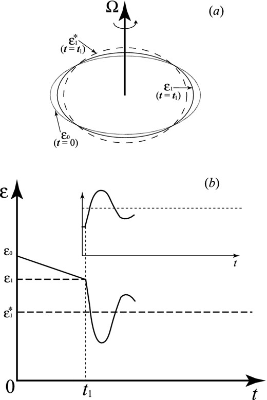
An illustration of the variable ε. The ellipticity of the star is exaggerated in this figure. The value of ε0 is the non-elastic-energy ellipticity (the ellipticity when the star became a solid). As the star spins down, the ellipticity of a Maclaurin ellipsoid becomes ε1*. However, as a solid star, its real ellipticity (ε1) cannot reach this value. Part (b) shows the change of ε parameter corresponding to the change of Ω during the glitch. A similar figure was first used by Peng & Xu (2008) as an illustration.
![The total energy release during the bulk-variable (type II) glitches and bulk-invariable (type I) glitches with amplitudes of 10−6 and 10−9. For the type I case, only the upper limit of energy release is shown and the real energy release will be reduced by a factor of A/[2(A + B)] (see equation 37 please). The Lennard–Jones interaction is applied as an approximation to work out the mass–radius relation (Lai & Xu 2009). There are two main factors in this approximation: the number of quarks in one cluster (Nq) and the depth of the potential (U0). The case of three-quark clusters with potential of 100 MeV (solid lines) and 18-quark clusters with potential of 50 MeV (dashed lines) are considered. It is also worth noting that the energy release during a type I glitch is related to the time intervals between two glitches. In this calculation, the glitch is thought to happen once per month and the spin-down power is calculated according to the observational data of Vela.](https://oup.silverchair-cdn.com/oup/backfile/Content_public/Journal/mnras/443/3/10.1093/mnras/stu1370/2/m_stu1370fig2.jpeg?Expires=1716407206&Signature=STp-8o37zusroZXgZRAacuXXkxMipC5qJWS7uNsyG9lG2kVxBsE5G5QyC1ZDxDjiClVXWyjL~kopSSD9pBfNGaZbPtL1-8yZPXBHkwwkPchDmhl1s0moimezH7DIydpsUV8rjj7cDJE1CTmWFn8ApEqFF2dvovI409OgC8W7Qo8RZVMu~6qdQQ5U0ph~wvm1BlxwYFfp9PqPdiT9fRrfVEhIwIO74JiUGJB7QR9xbGINabmaRX~rqz1XHCOoNKVkWwbERBC4ne5f4K8cHTUuqCPqkqbIhZhfv96L~rMnazZPyvIx~5lHZZoJuKiw6256GAGSpFZpGeLN~h4C9kcmWw__&Key-Pair-Id=APKAIE5G5CRDK6RD3PGA)
The total energy release during the bulk-variable (type II) glitches and bulk-invariable (type I) glitches with amplitudes of 10−6 and 10−9. For the type I case, only the upper limit of energy release is shown and the real energy release will be reduced by a factor of A/[2(A + B)] (see equation 37 please). The Lennard–Jones interaction is applied as an approximation to work out the mass–radius relation (Lai & Xu 2009). There are two main factors in this approximation: the number of quarks in one cluster (Nq) and the depth of the potential (U0). The case of three-quark clusters with potential of 100 MeV (solid lines) and 18-quark clusters with potential of 50 MeV (dashed lines) are considered. It is also worth noting that the energy release during a type I glitch is related to the time intervals between two glitches. In this calculation, the glitch is thought to happen once per month and the spin-down power is calculated according to the observational data of Vela.
In the calculation of the type I glitches, we suggest that the ellipticity of pulsar reaches the critical Maclaurin ellipticity (ε0) at the end of each glitch, which means all the elastic energy is released during the glitch. However, there could be some cases that only part of the elastic energy is released in a glitch (Peng & Xu 2008), i.e. maybe only the surface of the star breaks up and changes its shape. So our result is only an upper limit of real energy release during a type I glitch.
It is clear that even the largest bulk-invariable glitch (δν/ν ∼ 10−6) releases no more energy than 1038 erg. While a δν/ν ∼ 10−9 bulk-variable glitch is six orders of magnitude more energetic.
4 DISCUSSIONS AND CONCLUSIONS
The reason why the energy release during a type I and a type II starquake are different is the fact that the matter near the equator contributes to most of the moment of inertia. A global collapse happens during a type II starquake. The matter near the polar region can hardly reduce the pulsar's moment of inertia when collapse. Actually, most of collapsed matter could not contribute to the spin-up of the pulsar when it releases gravitational energy. Therefore, a bulk-variable type II starquake seems more energetic. However, for a type I starquake, what really changes is the matter distribution. A type I starquake could be regarded as a transport of matter from equator to the pole. It is true that gravitational energy can also release because the radius at the polar region is less than that at the equator, but reducing moment of inertia is much more efficient. This is the reason why less energy releases but the star spins up a lot during a type I starquake. Additionally, it has been discussed that the time-scale for the elastic energy built up in a type I starquake is longer than that in a type II starquake. And the quake may happen in different position in the star. These will also lead to quite different manifestations of energy release (Tong & Xu 2011). Observationally, glitches have been classified into two sorts according to the radiative properties which is quite similar to what we have done in this paper (Tong 2014). The two types of starquakes in a solid quark star model discussed above can account for the two types of glitches in observation.
As with the trigger of the starquake, we think that accretion should be the key factor for a type II glitch. As mentioned above, elastic energy develops substantially when a solid star gains mass and thus gravity (Xu et al. 2006). We may expect that type II glitches are most likely to happen in AXP/SGRs since (1) they are spinning slowly and (2) accretion would be possible there (Chatterjee, Hernquist & Narayan 2000) and observation hints the existence of disc (Wang, Chakrabarty & Kaplan 2006). It is also consistent with the ‘quark star/fallback disc’ model in which AXP/SGRs are thought as solid quark stars surrounded by fallback discs (Xu et al. 2006; Tong & Xu 2011). However, for normal pulsars, such as Vela/Crab pulsars, the compact objects rotate relatively faster, and the ellipticity change should be considerably important during the evolution. It is also worth noting that type II glitches could occur not only on solid quark stars with large masses. Because of gravity, real stellar radius is always smaller than that given by M ∼ R3 law. Certainly elastic energy is accumulated whenever the accretion happens. Another factor of accumulating anisotropic pressure distributed inside solid matter could be the temperature effect (Peng & Xu 2008).
For previous starquake-induced glitch models, it is known that large glitches on Vela pulsar happen so frequently that the stress built up in the star is smaller than required. However, in our model, large glitches on Vela do not necessarily imply that large amount of energy is accumulated. What really matters is the initial ellipticity of Vela (i.e. the ellipticity when Vela became solid). By suggesting the rotation period of Vela was 4 ms when it solidified, the initial reduced ellipticity (ε ∼ 0.01) would be large enough for Vela to suffer more than 10 000 glitches with Δν/ν ∼ 10−6 during its lifetime. It may infer a short time-scale before the solidification of the newly born pulsar. According to the theoretical conditions and observational hints (Xu 2003; Dai, Li & Xu 2011), a quark cluster star with the density of two times nuclear density is most likely to solidify at the temperature of T ∼ 0.5 MeV. It happens at about 1000 s after the formation of the star, which is reasonably short. We also need a large constant of B (B ∼ A) in this model so that considerable part of ellipticity decrease happens during the glitch.
A real glitch may consist of both types, which means when the radius of an AXP/SGR shrinks, there could also be a trend that part of the matter flow to the polar region. This could be a reason why the observed energy of the outbursts is much less than that we predict for a type II glitch. Another reason is that the majority of the energy release is taken away by neutrino emission. The energy loss due to gravitational radiation depends on the detailed behaviour of the stellar oscillation during and after the glitch. However, gravitational radiation is expected to be weak for a type I glitch because the total energy release is negligible.
In conclusion, it is found that two types of starquakes could occur in a solid quark star as it evolves: type I (bulk invariable) and type II (bulk variable). The total stellar volume decreases abruptly during a type II starquake, but it is conserved for type I even if stellar elipticity changes discontinuously. Consequently, a pulsar may spin-up suddenly, observed as a glitch, and it is then evident that there are two types of glitches caused by each type of starquake in a solid quark star model. A type II glitch could be energetic enough for us to detect X-ray emission even if the glitch amplitude of Δν/ν would be as small as 10−9. For a type I glitch, no X-ray enhancement could be detected even for a large glitch of Δν/ν ∼ 10−6.
We would like to thank the pulsar group of PKU for useful discussions. This work is supported by National Basic Research Program of China (2012CB821800), National Natural Science Foundation of China (11225314 & 11103021) and XTP project XDA04060604.
