


Summary
Numerical modelling of seismic wave propagation, considering soil nonlinearity, has become a major topic in seismic hazard studies when strong shaking is involved under particular soil conditions. Indeed, when strong ground motion propagates in saturated soils, pore pressure is another important parameter to take into account when successive phases of contractive and dilatant soil behaviour are expected. Here, we model 1-D seismic wave propagation in linear and nonlinear media using the spectral element numerical method. The study uses a three-component (3C) nonlinear rheology and includes pore-pressure excess. The 1-D–3C model is used to study the 1987 Superstition Hills earthquake (ML 6.6), which was recorded at the Wildlife Refuge Liquefaction Array, USA. The data of this event present strong soil nonlinearity involving pore-pressure effects. The ground motion is numerically modelled for different assumptions on soil rheology and input motion (1C versus 3C), using the recorded borehole signals as input motion. The computed acceleration–time histories show low-frequency amplification and strong high-frequency damping due to the development of pore pressure in one of the soil layers. Furthermore, the soil is found to be more nonlinear and more dilatant under triaxial loading compared to the classical 1C analysis, and significant differences in surface displacements are observed between the 1C and 3C approaches. This study contributes to identify and understand the dominant phenomena occurring in superficial layers, depending on local soil properties and input motions, conditions relevant for site-specific studies.
1 INTRODUCTION
In the last decades, local site conditions have emerged as one of the main components that govern the seismic ground motion. Numerous studies have shown that the ground response at a specific site is strongly controlled by the local soil properties, like the impedance contrast between the bedrock and overlying layers (e.g. Kramer 1996), constitutive material model and incident motion complexity (e.g. Gélis & Bonilla 2012, 2014), and site geometry (e.g. Graves 1993; Moczo et al. 1996; Olsen & Archuleta 1996).
Laboratory experiments performing cyclic loading on soil samples have shown shear modulus degradation and increasing damping for increasing shear deformation (e.g. Seed & Idriss 1969; Vucetic & Dobry 1991; Darendeli 2001). This means reduction of the wave speed and increase of the energy dissipation of the propagation media, respectively. In addition, results from laboratory tests, involving pore-pressure measurements on cohesionless saturated soils, exhibit contractive and dilatant behaviour; phenomena related to flow liquefaction and cyclic mobility (Ishihara 1996).
Furthermore, many observations from past earthquakes, for example, the 1994 Northridge, 1995 Hyogo-Ken Nanbu (Kobe), 1999 Chi Chi, 2000 Tottori, 2011 Tohoku and 2015 Gorkha (Nepal) earthquakes show that nonlinear soil response is pervasive during strong motion (Aguirre & Irikura 1997; Field et al. 1997; Pavlenko & Irikura 2003; Roumelioti & Beresnev 2003; Kokusho 2004; Bonilla et al. 2011; Rajaure et al. 2016). In particular, in the presence of cohesionless saturated material having predominant dilatant behaviour, observed accelerograms present high-frequency spiky waveforms leading to large acceleration pulses (Iai et al. 1995; Bonilla et al. 2005, 2011; Laurendeau et al. 2016).
Numerical modelling is an efficient tool to highlight the influence of different parameters governing site effects. Traditionally, nonlinear soil behaviour has been approximated by the equivalent linear method (Schnabel et al. 1972). This method has widely been used because only the shear modulus and damping curves as a function of shear strain are needed and low computational effort is required (Bardet 2000; Kausel & Assimaki 2002). However, for strong input motion, the equivalent linear method is found to overestimate the material strength (Joyner & Chen 1975; Yoshida & Iai 1998; Hartzell et al. 2004; Stewart & Kwok 2008; Kaklamanos et al. 2015). Conversely, nonlinear soil constitutive models, based on the stress–strain history of cyclic behaviour, have successfully been applied to 1-D wave propagation (Lee & Finn 1978; Pyke 2000; Hashash & Park 2001; Bonilla et al. 2005). There are also extensions to 3-D nonlinear models (i.e. Mroz 1967; Dafalias & Popov 1977; Prévost 1977; Wang et al. 1990). Yet, many of these multidimensional models are based on numerous parameters, making their use sometimes prohibitive. The Masing–Prandtl–Ishlinskii–Iwan (MPII) model of Iwan (1967) (as adopted in Joyner & Chen 1975; Joyner 1975; Gandomzadeh 2011; Santisi d'Avila et al. 2012; Pham 2013) is an interesting alternative to model material nonlinearity. Modelling is done by a set of nested yield surfaces consisting of simple elastic springs and Coulomb friction elements. It requires only the shear modulus reduction as a function of shear strain, which is readily obtained from laboratory data or from the literature for a wide range of soil classes (Vucetic & Dobry 1991; Electric Power Research Institute 1993; Ishibashi & Zhang 1993; Darendeli 2001).
Another important aspect is the choice of the numerical method to solve the wave equation. It influences the computational efficiency of numerical modelling in terms of precision of the solution and computational cost. One of the most commonly used methods to solve the seismic wave equation is the finite differences method (FDM), which has been extensively developed by many researchers (Madariaga 1976; Virieux 1986; Levander 1988; Graves 1996; Saenger et al. 2000; Moczo et al. 2002). Soil nonlinearity has been modelled in several studies of 1-D/2-D seismic wave propagation using FDM with no pore pressure effects, also known as total stress analysis (i.e. Joyner 1975; Joyner & Chen 1975; Gélis & Bonilla 2012, 2014). Yet, FDM has also proven to be robust when pore pressure is taken into account. This kind of analyses are known as effective stress analysis and they are the only ones capable of modelling observed accelerograms strongly affected by dilatant/contractive soil behaviour (i.e. Pyke 2000; Bonilla et al. 2005). Although its implementation is relatively straightforward, FDM can present some limitations in modelling non-planar topographies or complex interfaces inside the medium.
A different approach, which facilitates the adaptation of mesh to complex geometries in 3-D, is the finite element method (FEM; Lysmer & Drake 1972; Marfurt & Kurt 1984; Bielak et al. 2005). It has been used in many studies where nonlinear soil assumption is made for –one-component (1C) and 1-D–three-component (3C) seismic wave propagation (e.g. Iai et al. 1995; Hashash & Park 2001; Borja et al. 2002; Gandomzadeh 2011; Santisi d'Avila et al. 2012; Gandomzadeh 2011; Pham 2013). However, one limitation of FEM is that the global mass matrix needs to be inverted at each time step, which results in longer computation times. Such heavy computations could be avoided by lumping the mass matrix to turn it into a diagonal matrix. Yet, such a procedure may introduce numerical dispersion (Hinton et al. 1976; Mullen & Belytschko 1982; De Basabe & Sen 2007). Combining different methods such as FDM and FEM has also been proposed (e.g. Moczo & Kristek 2005; De Martin et al. 2007; Ducellier & Aochi 2012).
As a promising alternative technique, the discontinuous Galerkin finite element method (DGM), based on exchange of numerical fluxes between adjacent elements, provides high order direct solution (Käser & Dumbser 2006; Delcourte et al. 2009; Etienne et al. 2010; Peyrusse et al. 2014). Recently, DGM has been used in 1-D wave propagation modelling in nonlinear media (e.g. Mercerat & Glinsky 2015; Mercerat et al. 2016; Régnier et al. 2016).
Another high-order finite element method is the spectral element method (SEM). It has been used in Geophysics for many years for seismic wave propagation modelling (Madariaga 1976; Faccioli et al. 1997; Komatitsch & Vilotte 1998; Seriani 1998; Ampuero 2002; Festa & Vilotte 2005; Mercerat et al. 2006; Delavaud 2007; Smerzini et al. 2011). It provides easiness of mesh adaptation to complex geometries with higher precision than finite differences and low-order finite element methods. Numerical algorithms of the spectral element method considering 1-D and multidimensional plasticity theory have been used in engineering models (Leroy 2011). Some recent studies using SEM for seismic wave propagation also take into account nonlinear soil behaviour (i.e. Stupazzini & Zambelli 2005; Di Prisco et al. 2007; Stupazzini et al. 2009; He et al. 2016). Moreover, SEM was used in studies of seismic wave propagation in nonlinear crustal fault zones (Lyakhovsky & Hamiel 2009; Xu et al. 2012; Gabriel et al. 2013; Xu et al. 2015; Thomas et al. 2017).
In this work, we develop a numerical tool to study soil nonlinearity respecting geomechanical characteristics of the medium and considering the excess-pore pressure development effects on soil behaviour. We exploit the numerical advantages of SEM regarding precision and mesh adaptability to various medium properties. This advantage provides relatively cheaper computational times compared to other numerical methods having higher number of elements reaching the same accuracy (De Martin 2010). As for the nonlinear soil constitutive model, we use MPII model of Iwan (1967). In this approach, the total material damping is modelled through a combination of viscoelasticity and hysteretic behaviour as suggested by Assimaki et al. (2011) and Gélis & Bonilla (2012, 2014). For the purpose of modelling pore-pressure effects, we follow the formulation of Iai et al. (1990), which relates pore-pressure changes to the cumulative shear work (total shearing) produced during wave propagation. This empirical relation needs several parameters that can be obtained in the laboratory data or earthquake inversion analyses (Iai et al. 1990, 1995; Bonilla et al. 2005; Roten et al. 2013, 2014).
In this paper, we first present the 1-D–3C SEM code development. We then show the verification using the nonlinear and viscoelastic rheologies for 1C shear wave propagation by reproducing the computations performed in the PRENOLIN project (Mercerat et al. 2016; Régnier et al. 2016) and in previous studies (Peyrusse et al. 2014; Martino et al. 2015). Second, we study the impact of taking into account the multicomponent wave propagation on the development of soil nonlinearity compared to the traditional 1C analysis. Lastly, we model the acceleration–time histories of the 1987 Superstition Hills earthquake recorded at the Wildlife Refuge Liquefaction Array (WRLA). A sensitivity analysis is performed to assess the influence of soil rheology and the number of components propagating in the 1-D medium (1C versus 3C) for the same site.
2 NUMERICAL SCHEME AND CONSTITUTIVE MODELS
In this section, the spectral element method is briefly presented. Then, the constitutive models are given for viscoelasticity and nonlinearity of the medium.
The spectral element approximation is based on the decomposition of the domain into overlapping elements Ωe (segments in 1-D, quadrangles in 2-D and hexahedra in 3-D). In each element Ωe, Gauss–Lebatto–Legendre (GLL) integration points are defined. Lagrange polynomials are then chosen to define an orthogonal basis, which enables the SEM to have a spectral convergence, making it a very precise numerical method (Festa & Vilotte 2005; Delavaud 2007). In our case, the equation of wave propagation follows the velocity-stress formulation. The time discretization follows the leap-frog scheme. The time step has to verify the Courant–Friedrichs–Lewy (CFL) condition to ensure the stability of this time-marching solver. We use 0.3 as the controlling value of CFL for all the applications in this paper. Here the definition of the controlling value is adopted from Delavaud (2007), in which the computed CFL number is based on minimum spacing between GLL nodes in the spectral element. The element size d is chosen by respecting the formula d ≤ λminN/ppw, where λmin is the shortest wavelength propagating in the medium, N is the polynomial degree and `ppw' is the number of grid points per wavelength, to avoid artificial wave dispersion (Seriani & Priolo 1991). In the aforementioned study, the authors show that the use of ppw = 5 is needed for a wave propagation without numerical dispersion, while finite difference and low-order finite element methods require values between 15 and 30.
The 1-D–3C nonlinear SEM code has built-in different soil rheologies such as linear, viscoelastic and visco-elastoplastic behaviour. In a viscoelastic medium, attenuation is quantified by using the quality factor Q (Aki & Richards 2002; Moczo & Kristek 2005). The convolution relating stress and strain in the frequency domain in viscoelasticity theory is converted into a differential form by means of additional memory variables to model the viscoelastic attenuation, corresponding to a Generalized Maxwell Body (Day & Minster 1984; Emmerich & Korn 1987; Day & Bradley 2001). In this study, we choose the approach proposed by Liu & Archuleta (2006) that approximates a constant Q between 0.01 and 50 Hz by eight mechanisms of pre-calculated memory variables. In the 1-D–3C SEM code, the memory variables and the viscous modulus corresponding to Qp and Qs values at a given reference frequency fr are utilized, respectively. We recall that the total energy dissipation in the soil is modelled as the sum of viscoelastic attenuation and hysteretic attenuation similarly to Assimaki et al. (2011) and Gélis & Bonilla (2012, 2014).
To model the excess-pore pressure generation under cyclic loading we follow the study of Iai et al. (1990). In their study, the authors relate the cumulative shear work and the mean effective stress as it has been observed in experimental data (Towhata & Ishihara 1985). The time evolution of the parameters in this relation is called liquefaction front. The liquefaction front represents the envelope of stress points at equal shear work in normalized stress space relating the applied normalized deviatoric stress r to current normalized mean effective stress S (the normalization factor is the initial mean effective stress). In this stress plan, the soil is characterized by two limits during cyclic loading. The first one is the transition between contractive and dilatant behaviours and the second one is the rupture limit. The boundaries of these two limits are called phase transformation and failure lines, respectively (Fig. 1). The 1D-3C SEM code couples the nonlinear MPII model with the model of Iai et al. (1990) in presence of liquefiable soil layers. At each time step, the increment of the cumulative plastic shear work and the current effective stress corresponding to the matrix of current total stress are computed. The backbone curve of the soil (hyperbolic curve of eq. 1) is reconstructed according to the current effective stress. Appendix A2 describes all equations and parameters related to the liquefaction front model.
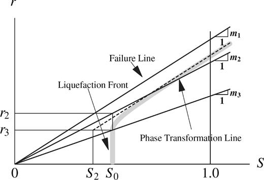
Schematic plot of liquefaction front model in normalized stress space. S holds for normalized mean effective stress and r is the normalized deviatoric stress (after Iai et al. 1990).
The medium is divided into elements for the wave propagation modelling. The mesh for a nonlinear medium is created based on the shortest wavelength. Since we do not have an adaptive meshing in time and space, the procedure we follow is to suppose that the minimum shear wave velocity during the simulation does not become less than one-fourth of the initial shear wave velocity (corresponding to the reduction of shear modulus to one-sixteenth of the initial shear modulus). We check at the end of the simulation whether the computed strains are compatible with the a priori shear modulus reduction to see if the solution is stable (e.g. Gélis & Bonilla 2012). If the minimum shear modulus during the simulation becomes less than one-sixteenth of the initial shear modulus, we further refine the meshing by a factor of 2. For all the nonlinear models in this study, 50 springs of MPII model are used. In Appendix B, the influence of number of GLL nodes and Iwan springs on the precision of SEM solution in nonlinear media is shown for one of the models used in this paper.
3 VERIFICATION OF VISCOELASTIC AND NONLINEAR MODELLING
Different tests are performed to compare SEM results with other numerical methods for the purpose of verification. First, the verification of viscoelasticity implementation is performed followed by the one considering nonlinear rheology. The wave propagation is computed using only one shear component in both cases.
To verify the viscoelasticity implementation, we perform 1-D–3C SEM computations of a soil profile in Rome, Italy from Martino et al. (2015) study. We then compare these results with those used in Martino et al. (2015). The 1-D Rome model is composed of 14 soil layers overlying bedrock (Table 1). The soil profile includes velocity inversions, for example layer 4 has a higher velocity than layer 5. The reference frequency fr is set to 1 Hz for all layers. Such a complex model allows to track small differences between numerical methods up to high frequencies. The free surface is modelled by a Neumann condition. Elastic rock boundary at bottom is modelled by absorbing layers of Classical Perfectly Matched Layers (C-PML). The input motion used is the same as in Peyrusse et al. (2014), a synthetic Gaussian wavelet low pass filtered below 14 Hz. The velocity–time history and corresponding Fourier amplitude of the input motion (after filtering) are shown in Fig. 2. A mesh corresponding to a resolution of 20 Hz and a 4th polynomial order (5 GLL points per element) is used. The element size varies from 2.5 to 16 m and a maximum number of two elements are used on each layer. Minimum distance between GLL points of elements changes from 0.4375 to 2.8 m. The time step is set to 2 × 10⁻⁵ s. The source is located at a depth of 100 m. In Fig. 3, acceleration–time histories at the surface from SEM and the Haskell–Thomson (HT) methods are shown in the top panel. Both techniques give identical results, verifying the implementation of the attenuation in the time-domain computations. The lower panel of Fig. 3 shows the transfer functions obtained by SEM and HT. They are obtained by computing the spectral ratio (FFT) of surface with respect to input motions. Since the input energy is limited to 14 Hz, the results are shown up to this frequency limit. Given the complexity of the media, this good agreement between the results of all the methods demonstrates the correct implementation of viscoelasticity. Appendix C1 addresses the goodness-of-fit of these simulations.
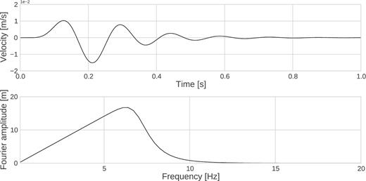
Velocity–time history (top) and Fourier amplitude (bottom) of the input motion used in Rome soil profile.
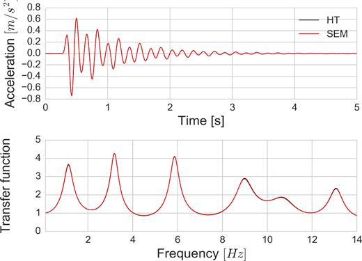
Comparison between acceleration–time histories at surface from SEM (in red) and HT (in black) (top) and transfer functions obtained with SEM (in red) and HT (in black) (bottom).
Soil properties at the Rome model.
| Layer | Thickness (m) | Vs (m s−1) | Vp (m s−1) | ρ (kg m−3) | Qs | Qp |
|---|---|---|---|---|---|---|
| 1 | 10 | 220 | 490 | 1835 | 100 | 200 |
| 2 | 6 | 239 | 523 | 1876 | 15 | 30 |
| 3 | 16 | 260 | 1480 | 1967 | 100 | 200 |
| 4 | 13.5 | 417 | 1760 | 1957 | 50 | 100 |
| 5 | 10 | 212.5 | 1235 | 1865 | 35 | 70 |
| 6 | 2.5 | 417 | 1760 | 1957 | 50 | 100 |
| 7 | 7 | 713 | 2560 | 2141 | 50 | 100 |
| 8 | 3 | 545 | 2125 | 2078 | 35 | 70 |
| 9 | 2.5 | 610 | 2379 | 2078 | 35 | 70 |
| 10 | 3 | 675 | 2632.5 | 2078 | 35 | 70 |
| 11 | 2.5 | 740 | 2886 | 2078 | 35 | 70 |
| 12 | 3 | 805 | 3139.5 | 2078 | 5000 | 10000 |
| 13 | 2.5 | 870 | 3393 | 2078 | 5000 | 10000 |
| 14 | 2.5 | 935 | 3646.5 | 2078 | 5000 | 10000 |
| Bedrock | 16 | 1000 | 3900 | 2078 | 5000 | 10000 |
To verify the implementation of the nonlinear soil model, we use one of the results obtained within the PRENOLIN project (Régnier et al. 2016). This project aims at comparing 1-D numerical wave propagation codes, having 21 international participating teams to model soil nonlinearity using canonical and real cases. One of the canonical cases of the project, the so-called P1 model, is used in this verification test. The free surface is modelled by a Neumann condition. At the bottom of the model, the rigid boundary is modelled by a Dirichlet condition with a zero velocity-field. In the P1 model, a single layer of soil is defined with a thickness of 20 m and a velocity of 300 m s−1 overlying a bedrock having a shear velocity of 1000 m s−1. A fourth-order polynomial degree (5 GLL points) is chosen for this model. A simple Ricker signal with a PGA of 0.93 m s−2 and a duration of 1 s, provided by the project, is imposed as input motion at the bottom of the discretized domain. In order to remove potential numerical noise with minimal loss of signal components, an acausal low-pass filtering is applied below 10 Hz by using a Butterworth filter before and after the simulation. The time step is set to 5 × 10⁻⁵ s. Elements of 5 m size are used in the model. The results obtained with SEM are compared to the results of another participant of the project, team EY, (Mercerat & Glinsky 2015; Régnier et al. 2016), who uses DGM code, where the MPII model is also implemented. Fig. 4 shows the stress–strain diagram for the point located at GL-9 m (left). Both methods show similar dynamic loading paths with negligible differences at the extreme values. Furthermore, due to soil nonlinearity, the material behaviour is no longer elastic and experienced values of shear strain become significant even under such simple input and site conditions.
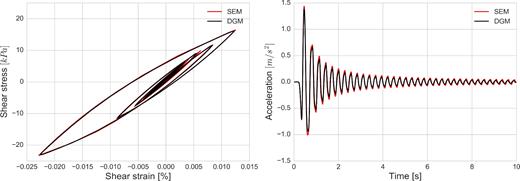
Stress–strain curves computed with SEM (in red) and DGM (in black) for the P1 model simulation using elastoplastic behaviour (left). Acceleration–time histories at the surface computed with SEM (in red) and DGM (in black) (right).
Another comparison between two methods is made on the computed time histories of surface acceleration, Fig. 4 (right). SEM results show slightly higher peak acceleration amplitudes than DGM, which could be related to possible differences between SEM and DGM numerical modelling. Yet, the results obtained with the two methods are in good agreement in terms of waveform and phase. Appendix C2 quantifies the similarity of these two simulations. Other comparisons between different numerical schemes using Iwan (1967) nonlinear model in 1-D seismic wave propagation can be found in Mercerat et al. (2016).
4 COMPARISON OF UNIAXIAL AND TRIAXIAL LOADING
In the 1-D–3C SEM code, the propagation can be computed using two shear components (x, y) and one compression component through the vertical axis (z), so that all the three components (x, y, z) can be considered in the calculations. Under multiaxial stress state, the loading is likely to lead to more energy dissipation and to result in a consequent plastification effect in the soil (Santisi d'Avila et al. 2012). In this section, we compare the nonlinear soil behaviour under uniaxial and triaxial loading without modelling pore-pressure excess. For this purpose, the previously used P1 model is used with the same input signal. The soil column is loaded in the x-direction only, so that the propagation is done for one shear component. For the triaxial loading, the same input signal is defined for all components (x, y, z). This configuration is not realistic, but it is only used for demonstration purposes. Fig. 5 (left) shows that the stress–strain curve at the middle of the soil follows the prescribed backbone curve under uniaxial loading; while the right figure shows that the soil deviates from the backbone curve under triaxial loading. Such behaviour indicates higher plastification that leads to loss of soil strength and change in deformation values in the soil with higher damping. Consequently, at the surface, resultant motion is stronger for uniaxial loading than triaxial loading (top panel of Fig. 6). From the initial seconds of simulation, the increase in attenuation is noticeable.
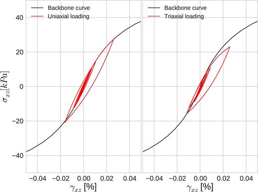
Comparison of the stress–strain curves for the P1 soil model under uniaxial (left) and triaxial loading (right). The backbone curve is shown in black.
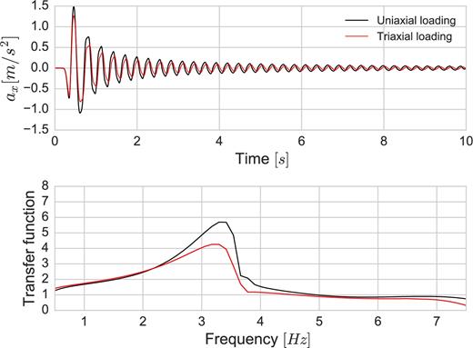
Surface acceleration–time histories (top) and transfer functions (bottom) for uniaxial (in black) and triaxial loading (in red).
Furthermore, a slight time shift of multicomponent simulation with respect to one-component computation is observed. Such an outcome is a consequence of higher nonlinearity corresponding to a lower shear modulus (lower wave speed) under triaxial loading. The transfer functions illustrate the impact of this higher nonlinearity under triaxial loading showing larger attenuation of maximum values (bottom panel of Fig. 6). The fundamental frequency is also slightly shifted from 3.5 Hz to 3.4 Hz.
The fact that soil becomes more plastic due to multiaxial loading even in cases where propagation is modelled for simple input motion shows the coupling of motion components in a 3-D nonlinear constitutive soil model. In more realistic conditions of input loading, plasticity arises mostly from double shearing because the horizontal components of the ground motion are usually larger than the vertical one. Yet, this can be a critical issue in the vicinity of the source where the vertical component may also be equal or larger than the horizontal ones. For this reason, additional energy attenuation with higher nonlinearity due to multiaxial loading should be taken into account for realistic modelling of seismic wave propagation.
5 VALIDATION OF THE 1-D–3C SEM CODE INCLUDING PORE-PRESSURE EFFECTS
5.1 The 1987 Superstition Hills Earthquake
To validate the 1-D–3C approach, we use data recorded at the WRLA, located on the floodplain of Alamo River in the Imperial Valley of California. The array was deployed by the United States Geological Survey (USGS) in 1987 with surface and downhole accelerometers (GL-7.5 m) and pore-pressure transducers at different depths. At WRLA, the pore-pressure changes were recorded together with the seismic motion generated by the ML 6.6 main shock of Superstition Hills on 1987 November 24 (Holzer et al. 1989).
We adopt the parameters of Bonilla et al. (2005) for the soil properties in our study (Tables 2 and 3). The velocity profile is composed of 4 soil layers. Vs and Vp correspond to shear and pressure wave velocities, respectively; ρ is the density, ϕf is the friction angle representing the failure line, and K0 is the coefficient of Earth at rest needed to compute the initial stress conditions. The water table depth is set to 2 m. The site is assumed to be initially isotropically consolidated and dilatancy parameters (ϕp, w1, p1, p2 and S1) are used for the third layer as proposed by Bonilla et al. (2005).
Soil properties at Wildlife Refuge Liquefaction Array after Bonilla et al. (2005).
| Layer | Description | Thickness (m) | Vs (m s−1) | Vp (m s−1) | ρ (kg m−3) | ϕf (°) | K0 |
|---|---|---|---|---|---|---|---|
| 1 | Silt | 1.5 | 99 | 249 | 1600 | 28 | 1.0 |
| 2 | Silt | 1.0 | 99 | 281 | 1928 | 28 | 1.0 |
| 3 | Silty sand | 4.3 | 116 | 1019 | 2000 | 32 | 1.0 |
| 4 | Silty sand | 0.7 | 116 | 1591 | 2000 | 32 | 1.0 |
Dilatancy parameters for the loose silty sand layer at the Wildlife Refuge Liquefaction Array (after Bonilla et al. 2005).
| ϕp (°) | w1 | p1 | p2 | S1 |
|---|---|---|---|---|
| 24.0 | 4.0 | 0.4 | 0.9 | 0.01 |
| ϕp (°) | w1 | p1 | p2 | S1 |
|---|---|---|---|---|
| 24.0 | 4.0 | 0.4 | 0.9 | 0.01 |
Dilatancy parameters for the loose silty sand layer at the Wildlife Refuge Liquefaction Array (after Bonilla et al. 2005).
| ϕp (°) | w1 | p1 | p2 | S1 |
|---|---|---|---|---|
| 24.0 | 4.0 | 0.4 | 0.9 | 0.01 |
| ϕp (°) | w1 | p1 | p2 | S1 |
|---|---|---|---|---|
| 24.0 | 4.0 | 0.4 | 0.9 | 0.01 |
5.2 Numerical model
Borehole wavefield at GL-7.5 m depth is used as input in the simulations. The strongest motion is recorded on the north-south direction with an amplitude of 1.60 m s−2, while the weakest motion is on the vertical direction with a PGA of 0.54 m s−2, Fig. 7. Hereafter, north–south component is symbolized by NS, east–west component by EW and vertical component by UD.
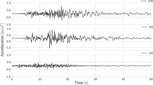
Acceleration–time histories recorded in the east–west (EW), north–south (NS) and vertical (UD) directions at GL-7.5 m depth of WRLA.
5.3 Results
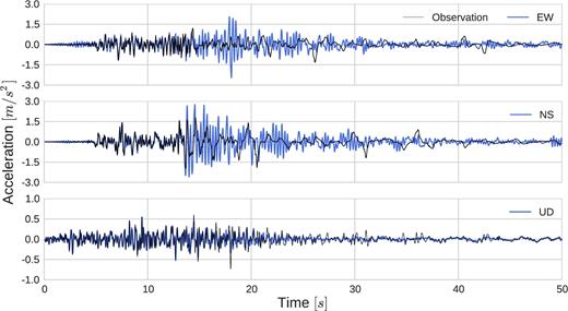
We compare the observed ground motion at the surface with the computed synthetics in the three directions. Fig. 8 shows the computed accelerations at the surface. After the first 13 s, the accelerograms show large dilatation pulses riding on a low-frequency carrier. Except for the slight phase differences on the NS component and some amplitude dissimilarities, the simulation is able to reproduce well the observed ground motion.
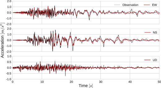
Comparison of surface acceleration–time histories between the results of effective stress analysis of SEM (in red) and real records (in black) for the WRLA site.
Moreover, a similar comparison is made between computed and observed velocity–time histories, Fig. 9. After 20 s, SEM solution and observation on the NS component exhibit slight phase and amplitude differences. Appendix C3 shows the goodness-of-fit analyses of SEM results with respect to observed acceleration and velocity–time histories, respectively.
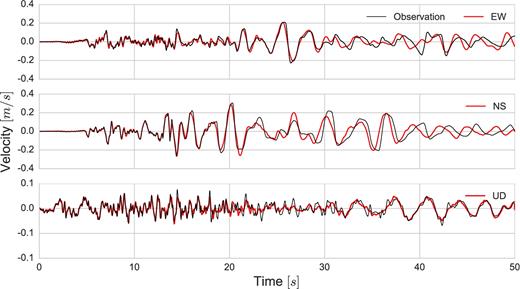
Comparison of surface velocity–time histories between the results of effective stress analysis of SEM (in red) and real records (in black) for the WRLA site.
The long period pulses in the horizontal components of the acceleration–time histories can be explained by the dilatancy changes in the liquefiable silty sand layer (GL-2.5 m - GL-6.8 m). Two points at different depths are chosen to see these changes. The first corresponds to a depth of GL-2.9 m, where pore pressure effects were recorded; and the second is located in the middle of the soil column. Fig. 10 shows the normalized deviatoric stress (r) as a function of the normalized current effective stress (S) for these two points (initial effective stress is used as normalization factor). A continuous decrease in effective stress is observed. At GL-4.0 m depth, the soil experiences dilatant behaviour by reaching the phase transformation line.
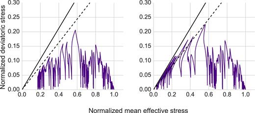
Stress space at GL-2.9 m (left) and GL-4.0 m (right), respectively. Solid and dashed lines represent the failure and phase transformation boundaries.
Moreover, the stress–strain curves are plotted for the same locations in Figs 11 and 12. At each depth, the decrease in effective confining stress can be remarked by slope changes of shear strength. Differently than GL-2.9 m, dilatancy at GL-4.0 m results in stress–strain loops for shear components having the classical banana shape, which is typical of softening and partial regain of soil strength due to successive changes in soil dilatancy. Maximum strain reached by the soil at this depth is close to 5 per cent. Strain values at depth GL-2.9 m are small due to the large attenuation of the incoming waves. Conversely,in the vertical component at either depth, the behaviour is close to elastic conditions. Such an outcome results from the fact that the bulk modulus is independent of soil dilatancy changes in this model. Such an assumption should be studied in the future, yet it produces good results when modelling the vertical wave propagation in this case.
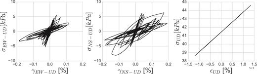
Stress–strain curves of EW-UD component (left), NS-UD component (middle) and UD component (right) at GL-2.9 m.
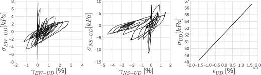
Stress–strain curves of EW-UD component (left), NS-UD component (middle) and UD component (right) at GL-4.0 m.
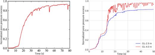
Furthermore, we compute the change of the pore-pressure excess inside the liquefiable soil layer. Fig. 13 displays at GL-2.9 m (left) and those computed at GL-2.9 m and GL-4.0 m (right), respectively. A sudden increase in pore pressure is seen after 13 s at both depths. Since the effective stress decreases more at GL-4.0 m, the pore-pressure excess reaches higher values than GL-2.9 m. Continuous changes in contractive-dilatant behaviour of the soil at GL-4.0 m is seen in the same figure by successive oscillations in pore-pressure values. As soil becomes contractive, pore pressure decreases, while it increases for dilatant soil behaviour. Such sudden changes in dilatancy, where stress path changes direction and effective stress increases with dilatant behaviour, are related to partial gain of strength and consequent spiky values in surface acceleration which take place after 13 s. Oscillations related to dilatant behaviour at GL-2.9 m in SEM solution have higher amplitudes compared to the recording. Although these differences are not significant to interpret the evolution of soil behaviour under excess-pore pressure development, the numerical solution could be improved by modification of parameters of the liquefaction front model. Indeed, the parameters used in this study have been determined for another constitutive model of soil nonlinearity (Iai et al. 1990; Bonilla et al. 2005). Also, triaxial loading condition leads the soil to higher nonlinearity, differently than the mentioned studies that used uniaxial loading condition. Furthermore, in Holzer & Youd (2007), the authors explained the continuous increase in pore-pressure excess and ultimate liquefaction process with the formation of surface waves (Love and Rayleigh waves) and consequent shearing in WRLA. Same authors stated the presence of surface waves in the input motion at GL-7.5 m, which suggests the importance of 2-D/3-D effects on the incoming wavefield that may increase the pore-pressure effects. However, the generation and lateral propagation of these surface waves cannot be accounted for our 1-D model.
Thus far, the influence of cyclic-mobility phenomenon in the 4.3 m thick silty sand layer is demonstrated and the spiky wavelets at surface are explained due to the sudden changes in pore pressure and dilatant behaviour of the silty sand layer. The good agreement between observed and calculated accelerations supports the nonlinear soil rheology used in this study. In the next section, a sensitivity study is carried out to highlight the effect of soil rheology and input loading (1C and 3C approaches) at WRLA.
5.3.1 Influence of material rheology on wave propagation
We investigate the influence of ignoring the excess-pore pressure development on the response of the WRLA soil column using a visco-elastoplastic analysis. Three components of the computed acceleration–time histories at the surface are compared between two approaches (with/without pore-pressure effects). Fig. 14 shows that signals are dominated by high-frequency motion in both shear components. The particular waveform observed after first 13 s in these components cannot be reproduced. Conversely, only few differences are noted between the calculated and observed vertical motions. Such an outcome arises from the fact that the constitutive equations lead to development of strong material nonlinearity mainly in the deviatoric plan. It is a drawback of the model since it will not be able to correctly model volumetric changes during cyclic loading. This aspect has to be improved in the future to correctly predict vertical settlements.
Surface acceleration–time histories for simulation without pore-pressure effects (in blue) and observation (in black) at the WRLA.
The effect of pore-pressure excess is also shown on the response spectra. Fig. 15 depicts the 5 per cent response spectra of the three components of surface acceleration for effective stress analysis (in red) and total stress analysis (in blue). A very strong peak around 3 Hz in the visco-elastoplastic analysis without pore-pressure excess is noted in both shear directions. This peak is significantly damped with the introduction of cyclic mobility in the third layer so that the results become much closer to the observations. In addition, at low frequencies (<1 Hz), the spectrum is amplified when excess-pore pressure is taken into account, which results in a better fit to the observation. As before, the vertical component remains unaffected by the presence or not of pore pressure.
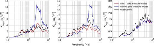
Comparison of response spectra between real records (in black), effective stress analysis of SEM (in red) and total stress analysis of SEM (in blue) for EW component (left), NS component (middle) and UD component (right).
These results reveal the importance of taking into account the correct soil constitutive model in surface-motion modelling. The response spectra of ground motion are strongly influenced by soil rheology in the frequency band of interest for Earthquake Engineering (0.1–10 Hz). Thus, for certain structures whose resonance frequencies fall into the low-frequency band, the design could exceed the safety limit if the rheological characteristics of the underlying media are not correctly taken into account. Such considerations enhance the importance of realistic hypothesis and good knowledge of the soil behaviour and properties during site-specific studies.
Furthermore, the depth profiles of maximum strain for the three components of total and effective stress analyses are compared in Fig. 16. A significant increase in strain values of the third layer is noted on the shear components for the simulation with excess-pore pressure development. The maximum soil strain reaches to 5 per cent on NS-UD component of shear strain (γNS-UD), while it does not exceed 0.2 per cent without pore-pressure excess. Concomitantly, as the strain increases in the third layer, an overall strain decrease is seen in other layers. In a highly nonlinear liquefiable soil layer, the incoming waves could be trapped under pore-pressure effects and such wave trapping could result in higher deformation in effective stress analysis compared to total stress analysis.
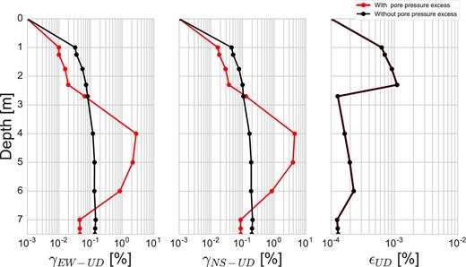
Comparison of maximum strain profiles as a function of depth between effective stress analysis of SEM (in red) and total stress analysis of SEM (in black) for EW-UD (left), NS-UD (middle) and UD (right) components.
5.3.2 Uniaxial versus Triaxial loading
Here, we compare the response of the soil column under uniaxial and triaxial loading conditions. In Section 4, we showed that the soil becomes more nonlinear due to multicomponent loading. In this section, we investigate this effect in a real model, in which pore-pressure excess plays an important role, using the real records for the site. For this purpose, we propagate only the NS component in uniaxial loading case. The comparison is made in the direction where the motion is the strongest.
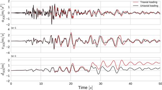
The results of acceleration, velocity and displacement time histories computed at the surface are shown in Fig. 17. In the first 13 s, the results are very similar between uniaxial and triaxial loading. Then, waves arrive later in triaxial loading than uniaxial loading. This phase difference indicates that the velocity of the media has further decreased under triaxial loading. Indeed, soil behaviour exhibits higher amplitudes and presents larger permanent displacements for the 3C computations compared to traditional 1C computations.
Comparison of maximum strain profiles as a function of depth between effective stress analysis of SEM (in red) and total stress analysis of SEM (in black) for EW-UD (left), NS-UD (middle) and UD (right) components.
Furthermore, the stress–strain loops at GL-4 m show more nonlinear and dilatant behaviour, producing higher deformations during triaxial loading compared to uniaxial loading (Fig. 18, left). Given the fact that soil is more nonlinear during triaxial loading, the effective stress decreases more rapidly resulting in earlier and stronger pore pressure rise. In consequence, the soil undergoes with more oscillations in the second half of the simulation (after 13 s) under triaxial loading (Fig. 18, right). Therefore, multiaxial interaction may become important for a realistic analysis on seismic wave propagation studies.
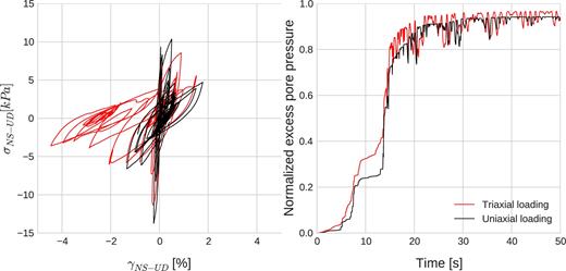
(left) Comparison of stress–strain curves between uniaxial (in black) and triaxial (in red) loading conditions for NS-UD components at GL-4.0 m; (right) Comparison of pore-pressure ratios at same depth.
6 CONCLUSIONS
This study shows the possibility of modelling wave propagation on nonlinear media including pore-pressure effects using SEM by coupling two different mechanisms. First, the nonlinear soil behaviour and second, the excess of pore pressure generation. These models need three elastic parameters (pressure and shear wave velocities and density), three parameters for viscoelastic attenuation (quality factors of P and S waves and reference frequency) and three parameters for nonlinearity (friction angle, cohesion and coefficient of Earth at rest). When excess-pore pressure development is taken into account, five parameters are required (ϕp, w1, p1, p2 and S1), which can be obtained by laboratory tests or strong motion inversion analyses.
The analyses of the 1987 Superstition Hills earthquake (ML 6.6) data, recorded at the WRLA, show:
Spiky behaviour of the recorded accelerograms is well reproduced by modelling the dilatant soil behaviour and related pore-pressure effect.
Nonlinear computation of the ground motion with no pore-pressure effects still overestimates high-frequency motion and underestimates amplification of low frequencies.
Triaxial loading conditions result in higher soil nonlinearity, which in turn produces a more rapid rise of the pore-pressure excess. Yet, deformations at depth in materials susceptible to excess-pore pressure generation could be quite large. For this reason, consideration of multiaxial interaction might sometimes be required for a realistic modelling of seismic wave propagation.
We have seen that this relatively simple model captures most of the physics observed in dilatant soils. This numerical tool is efficient and useful for a better understanding of the influence of soil-related phenomena on 1-D seismic wave propagation and multiaxial loading effects. Yet, solid–liquid phase interaction and fluid dissipation cannot be modelled. This aspect deserves further research in the future.
Acknowledgements
The authors would like to thank to Diego Mercerat, Aneta Richterova, Viet Anh Pham, Luca Lenti and Maria Paola Santisi d'Avila for their helpful comments and contributions and to Professor Susumi Iai for his instructive suggestions to the development of our work and this material when coupling the 3-D nonlinear model to his 3-D liquefaction front model. We would like to acknowledge Jean Paul Ampuero for both his careful review of this work and his preliminary collaboration with one of the co-authors (LFB) that demonstrated that SEM could handle nonlinear wave propagation. We are also grateful to the anonymous reviewer and the editor Professor Jörg Renner for their constructive comments that helped us to improve this paper.
REFERENCES
SUPPORTING INFORMATION
Supplementary data are available at GJI online.
Appendix A
Appendix B
Appendix C
Please note: Oxford University Press is not responsible for the content or functionality of any supporting materials supplied by the authors. Any queries (other than missing material) should be directed to the corresponding author for the paper.
