


Abstract
Macroseismic intensities are the only available data for most historical earthquakes and often represent the unique source of information for crucial events in the definition of seismic hazard. In this paper, we attempt at getting insight into source characteristics by reproducing the observed intensity field. As a test case, we study the source of 1908 Messina Straits earthquake (MW = 7.1), by testing three distinct fault models deduced from the analysis of geodetic data. Starting from the static slip distribution, we develop kinematic source models for the investigated fault and compute full waveform synthetic seismograms in a 1-D structural model, also accounting for anelastic attenuation. Then, we convert both computed peak-ground acceleration (PGA) and peak-ground velocity (PGV) to macroseismic intensity at 100 selected sites, by means of specific empirical relations for the Italian region. By comparing the original data separately with PGA- and PGV-based intensity fields, we discriminate among the tested faults and determine the best values for the investigated kinematic parameters of the source. We also perform a misfit analysis for the best source model, in order to investigate the dependence of the results on the selected parametrization. The results of the analysis indicate that among the tested models, the one characterized by an east-dipping fault, with strike-oriented NS slightly rotated clockwise, better explains the observed macroseismic field of the 1908 Messina Straits earthquake. Besides, the fracture nucleated at the southern end of the fault and ruptured northward, producing considerable directivity effects. This is in agreement with the published results obtained from the investigation of the historical seismograms. We also determine realistic values for the rupture velocity and the rise-time. Our study confirms the great potential of the macroseismic data, demonstrating that they contain enough information to constrain important characteristics of the fault, which can be retrieved by using complex source models and computing complete wavefield. Moreover, we also show that the simultaneous comparison of both PGA- and PGV-based synthetic macroseismic fields with the original intensities provides tighter constraints for discriminating among different source models, with respect to what attainable from each of them.
1 INTRODUCTION
Strategies for mitigating seismic risk are usually driven by what is depicted in hazard maps that, in turn, are generally based on a reliable knowledge of the source characteristics of past earthquakes and of their effects. However, the recognition of the seismogenic structures and the assessment of their seismic potential are also crucial. These latter are particularly critical when vulnerability and exposure are significantly high, as is the case in densely inhabited regions, where the correct identification of the active faults and the estimate of the associated seismic potential are of paramount importance.
Modern earthquakes are studied by means of dense networks, equipped with high-quality instruments, and the seismic source can be constrained by analysing quantitative data. On the other hand, large earthquakes are less frequent and, in areas where the return periods are of the order of hundreds of years or larger, instrumental recordings of such events do not exist or, sometimes, only a few historical seismograms are available at regional or teleseismic distances, making the analysis of the source very intricate and ambiguous. Therefore, the properties of the associated faults and the mode of stress release can only be deduced by careful and joint investigations of all the available data. Felt intensities are among these and, sometimes, they represent the only information on hand. Indeed, in the last decades, these latter have been used extensively to get insight into the source of old earthquakes and, since 40 yr ago at least (Shebalin 1973), techniques have been developed to derive quantitative estimates of source parameters from felt reports (see, for instance, Gasperini et al.1999 and references therein).
In order to image the source responsible for the observed intensities, some scheme is needed for the simulation of the macroseismic intensities produced by a given earthquake. Today, rapid scenarios are routinely generated by computing near real-time ground shaking maps (ShakeMap, Wald et al.1999; GRSMap, Convertito et al.2010). These integrate actual recorded data with ground motion predictions obtained by means of ground motion predictive equations (GMPEs). However, these techniques are only meant to provide a quick estimate of the potential damage for post-earthquake response and do not give information about the source characteristics.
In recent times, the demand for the development of specific earthquake's scenarios has increased notably. To this aim, sophisticated methods for computing realistic ground motion—in terms of broad-band waveforms generated by complex source models—have been implemented and several empirical relations to convert ground motion parameters to intensity scales have also been developed (Wald et al.1999; Faccioli & Cauzzi 2006; Faenza & Michelini 2010). Besides providing reliable estimates of the expected shaking for a specific event, these techniques may represent a useful tool for investigating the source of historical earthquakes by means of macroseismic data analysis, possibly giving indications about fault location and kinematics. As an example, in a recent paper, Imperatori & Mai (2012) investigated the ground motion dependence on the source and velocity model variations, demonstrating that, at intermediate and short wavelength, several features of the simulated ground motion are significantly sensitive to the details of the source, while the structural velocity model only affects long and intermediate periods. Albeit focused on the analysis of the broad-band ground motion, their study indicates that, as long as suitable relations linking ground motion to macroseismic scales are adopted, modelling intensity data by computing full waveform synthetic seismograms for complex source models is a powerful tool to investigate historical earthquakes. As a matter of fact, Emolo et al. (2004), who analysed the 1930 Irpinia (southern Italy earthquake), showed that even a qualitative comparison between original macroseismic data and intensities derived by converting ground motion parameters represents a viable technique to discriminate among different source models.
In their study, Imperatori & Mai (2012) used the 1908 Messina Strait earthquake as a test case, computing synthetic seismograms for several source models and crustal structures. However, we note that these authors adopted a fault plane whose orientation and mechanism are equal to those proposed by Amoruso et al. (2006). This event is somehow paradigmatic, representing a clear example of a major earthquake striking an area where only minor to light seismicity occurred since then and fundamental aspects related to the fault causing the event are still debated. The 1908 earthquake caused about 80 000 casualties, when the population was of about 140 000 in Messina and 45 000 in Reggio Calabria, respectively, on the west and east side on the Straits (Fig. 1). The source of the 1908 event has been questioned for several decades and, after more than a century of investigation, although there is a general agreement on the overall WNW–ESE extensional nature of the earthquake, several questions are still open. Recently, for instance, Aloisi et al. (2013) raised a major issue regarding the location and the dip orientation of the fault placing the fault top on the east side of the Straits, more that 20 km east of the previous determinations, and corresponding to a west dipping plane, opposite to what stated by most authors. However, their results have been recently criticized by De Natale & Pino (2014) and Cannelli et al. (2013) have shown that low-angle, eastward-dipping fault models provide a better fit to the post-seismic displacements recorded at the Messina station over the 15 yr following the earthquake, compared to westward-dipping fault models.
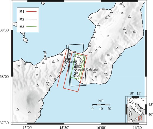
Geographic map showing the Messina Straits area. The 100 sites selected for the analyses presented in this study are also represented (triangles). The rectangles indicate the surface fault projection of the three investigated models for the source of the 1908 earthquake: M1 (Boschi et al.1989; red); M2 (Capuano et al.1988; De Natale & Pingue 1991; see text for details; black); M3 (Aloisi et al.2013; green), while the colour lines indicate the intersection of the upward prolongation of the fault with the Earth's surface.
By considering that the present population in the area is in excess of 700 000, with 500 000 in the Messina urban area and 190 000 in Reggio Calabria, with constructive quality of the buildings far from the optimal, the determination of a reliable fault model is not trivial nor it represents an academic dispute. In this study, we focused on the simulation of the macroseismic field associated with large events, by computing the broad-band ground motion produced by realistic seismic sources. Our main goal was the development of a procedure for the determination of source characteristics of historical earthquakes on the basis of the actual intensity data. We applied this technique to the source of the 1908 Messina Straits event and point at discriminating among distinct published fault models.
2 THE 1908 MESSINA STRAITS EARTHQUAKE
The Messina Straits earthquake stroke on 1908 December 28. In spite of its magnitude (MW = 7.1), not very large on a global scale, it caused extensive damage and a huge number of casualties, mainly because of the poor quality of the constructions. In the Messina and Reggio Calabria areas, 70–100 per cent of the buildings were destroyed. In terms of victims, it represents one of the most catastrophic earthquakes in the human history, being among the 20 deadliest seismic catastrophes (http://earthquake.usgs.gov/earthquakes/world/most_destructive.php). Several scholars from all over the world studied the event in the aftermath, but, due the lack of both physical models for the seismic source and advanced techniques for analysing data, not too much could be understood about the cause of the quake. Nevertheless, a considerable amount of data was gathered at that time, composed of macroseismic estimates and geodetic, seismological and mareographic measurements and recordings. These data have been repeatedly reanalysed in modern times by several researchers, starting from the pioneering work of Schick (1977), and a series of different models have been proposed for the causative fault (see the review by Pino et al.2009).
2.1 The macroseismic data
Many scientists went to the Straits to observe the effects of the earthquake and some of them gathered many observations about the damage, moving over an extended area. The most complete report was compiled by Baratta (1910), who run a considerable field survey and collected a notable number of detailed macroseismic data. He also used those data to determine two areas of main release, by analysing the direction of overturned bodies, as first made by Mallet (1862). The presently available data set of macroseismic observation regarding the 1908 event totals 800 points (Locati et al.2011) and is mainly based on the work of Baratta (1910). He also noted that the intensity data present some irregular features in the distribution, evidencing anomalies in zones that suffered intense damage already in previous earthquakes that indicate the occurrence of significant site effects. Overall, the macroseismic field covers a radius of about 200 km from the epicentre and displays a rough NS elongation, parallel to the Straits axis, reaching degree XI on the Mercalli–Cancani–Sieberg scale (MCS) in several locations along both sides of the Straits.
2.2 The source models
During several decades, a relatively consistent number of authors have proposed independent models of the earthquake's source. A thorough review is given by Pino et al. (2009) and here we only briefly outline the principal studies. The work made by Schick (1977) is the first study of the 1908 Messina Straits earthquake in the modern era. Based on seismological analyses and qualitative considerations on geodetic data, he proposed a source model represented by a steep normal fault, roughly parallel to the Sicilian coast and dipping westward. Then, Mulargia & Boschi (1983), who performed the first quantitative modelling of the original levelling data, found that a graben-shaped model with a couple of quasi-antithetic faults located, respectively, on the two sides of the Straits could account for the measured vertical static displacement of the ground. A few years later, Boschi et al. (1989) and De Natale & Pingue (1991) presented two distinct variable dislocation models derived by inverting levelling data. Both models were characterized by an about 45 km long fault, roughly oriented along the NS direction and dipping at low-angle eastward, with strike parallel to the Sicilian and to the Calabrian coast, respectively, and minor differences in the dip, and rake angles.
Pino et al. (2000) analysed regional seismograms, demonstrating that the fracture was prevalently unilateral, with northward propagation. They also showed that the retrieved moment rate is in very good agreement with the dislocation models of both Boschi et al. (1989) and De Natale & Pingue (1991), for a rupture starting at the southern edge of the fault and propagating to the north. Successively, this conclusion was implicitly corroborated by the epicentral location derived by Michelini et al. (2005) indicating that the earthquake nucleated in southern part of the Straits, approximately in correspondence of the southern edge of the Boschi et al. (1989) and De Natale & Pingue (1991) faults.
The model published by Amoruso et al. (2002) displays significant dislocation on a definitely longer fault plane, still dipping eastward and slightly rotated counter-clockwise with respect to that proposed by De Natale & Pingue (1991). As shown by Pino et al. (2009), the main features of the Amoruso et al. (2002) variable dislocation model are very similar to that of Boschi et al. (1989) and De Natale & Pingue (1991) ones in the common central area. On the other hand, unlike the previous recent models, the source proposed recently by Aloisi et al. (2013) is characterized by a fault located on the Calabrian side and dipping 60° westward, with surface projection almost not intersecting the Straits. It also displays a smooth slip distribution very dissimilar from the others, which are characterized by shorter wavelength details.
In order to select the models to test in our analysis, we considered the most reliable sources, based on the elements discussed by Pino et al. (2009), Amoruso et al.2010 and Pino et al. (2010). Therefore, we chose the models developed by Boschi et al. (1989) and De Natale & Pingue (1991). In addition, we also included the source obtained by Aloisi et al. (2013), representing a completely different solution and, notably, implying substantial repercussions on the evaluation of the seismic risk in the source area, if validated.
3 MODELLING OF INTENSITY DATA
Macroseismic data do not represent quantitative estimates of the ground shaking and cannot be directly modelled. Synthetic intensities are obtained by converting other ground motion measures such as peak-ground motion parameters. Especially for large magnitude earthquakes, reliable modelling of the macroseismic field requires the use of extended fault geometries and appropriate structural velocity models. Most analyses adopt simplified sources, with uniform slip distribution on the fault surface (e.g. Gasperini et al.1999), sometimes introducing directivity effect by considering a Haskell source model (e.g. Pettenati & Sirovich 2007). In the present study, in order to test more realistic sources, we used complex slip distributions and circular rupture propagation from a single nucleation point. We selected a few published fault geometries and, for each of them, we computed several sets of full waveform synthetics, by testing a number of distinct locations for the nucleation point and different realizations of slip distribution, rise-time, and rupture velocity. Thus, we estimated peak-ground velocity (PGV) and peak-ground acceleration (PGA) as the largest value on both horizontal components of the respective synthetics. By using the empirical relations proposed by Faenza & Michelini (2010) that are actually used to produce ShakeMaps in Italy (Michelini et al.2008), we converted PGV and PGA obtained for each source realization to MCS intensity. Then, in order to discriminate the best fitting source, we compared the results with the observations. Besides the evaluation of the simulated peak-ground motion values against the predictions obtained from a specific GMPE, as done for instance by Imperatori & Mai (2012), we compared the simulated MCS intensities directly with the observation at 100 selected localities.
We chose the sites by covering the area of interest with a circular grid, centred on the instrumental epicentre, with spacing of 10° in azimuth and 12 km in distance, enclosing sites up to a distance of 108 km. Next, we selected two random points for each areal bin containing two points at least and repeated the procedure a hundred times. Thus, by visual inspection, we chose the one with the most uniform azimuthal distribution (Fig. 1). This choice ensures higher sampling at short distances, where intensity is expected to be larger and to attenuate quickly.
3.1 Propagation modelling
Fault plane geometry, depth of the fault top (DFT) and focal mechanisms of the three tested models (see text for references).
| Model | L (km) | W (km) | DFT (km) | Strike (°) | Dip (°) | Rake (°) |
|---|---|---|---|---|---|---|
| M1 | 45 | 18 | 3 | 11 | 29 | −90 |
| M2a | 45 | 24 | 3 | 349 | 42 | −121 |
| M3 | 29 | 12 | 0.171 | 188 | 60 | −77b |
| Model | L (km) | W (km) | DFT (km) | Strike (°) | Dip (°) | Rake (°) |
|---|---|---|---|---|---|---|
| M1 | 45 | 18 | 3 | 11 | 29 | −90 |
| M2a | 45 | 24 | 3 | 349 | 42 | −121 |
| M3 | 29 | 12 | 0.171 | 188 | 60 | −77b |
1-D structural model used for the Green's functions computation
| Depth (m) | VP (m s−1) | VS (m s−1) | ρ (g cm−3) | QP | QS |
|---|---|---|---|---|---|
| 0 | 4000 | 2300 | 2393 | 817 | 363 |
| 500 | 4500 | 2600 | 2462 | 817 | 363 |
| 2500 | 4800 | 2700 | 2505 | 817 | 363 |
| 4300 | 5300 | 3100 | 2583 | 817 | 363 |
| 6200 | 6000 | 3500 | 2717 | 817 | 363 |
| 12 200 | 6200 | 3600 | 2761 | 817 | 363 |
| 18 200 | 6400 | 3700 | 2808 | 817 | 363 |
3.2 Source modelling
We investigated three different published fault geometries, all derived from the analysis of the historical levelling data. The first model was proposed by Boschi et al. (1989). The second is a slightly modified version of the one by De Natale & Pingue (1991), derived by using their slip distribution and the focal mechanism published by Capuano et al. (1988). This latter is very similar to the one by De Natale & Pingue (1991), with planes orientation differing by only a few degrees. The third was recently published by Aloisi et al. (2013; hereinafter indicated as M1, M2 and M3, respectively). The first two are almost comparable, while the third one displays very different fault plane dimension and dip orientation. The main features of three models are listed in Table 1 , while their surface projections are shown in Fig. 1. As remarked by Pino et al. (2009), the slip distributions of M1 and M2 are substantially similar, with three 7–8-km-large asperities, approximately located at half-width of the fault plane, and maximum slip amplitude of about 3.5 m.
On the other hand, a rather different dislocation map characterizes M3, which displays only large-scale features with an absolute maximum on the lower southern corner of the fault. As obvious, from the point of view of the ground motion, these fault models only account for the static properties of the source, whereas our main interest is the simulation of high-frequency parameters (PGA and PGV) to derive macroseismic intensities. Thus, it is necessary to introduce a kinematic rupture model.
In the adopted simulation scheme, each fault is modelled as a plane surface and is discretized in elementary subfaults by using a regular grid with node distance of 2 km along both the strike and dip directions. Each subfault is allowed to slip once, when reached by a circular rupture front, radiated from a single nucleation point. We selected a boxcar source time function.
Starting from the slip distribution of M2, we considered the along-strike maximum dislocation as plotted by Pino et al. (2000; green curve in the upper panel of Fig. 2), SMAX(l). We first discretized the curve by using the same step size as the one assumed for the fault grid (2 km), obtaining the function SMAX(n), with the integer n identifying the horizontal distance index. Then, we assigned to each subfault located at n a slip value randomly extracted from the interval SMAX(n) ± 25 per cent. Finally, we tapered and scaled the resulting slip map by a uniform factor, to constrain the total seismic moment to be M0 = 5.6 × 10¹⁹ Nm (derived by Pino et al.2000) for the three fault models. Therefore, all the maps of slip contain three main patches characterized by different maximum slip values and areal extent. Note that starting from the same along-strike maximum dislocation function for the three fault models did not affect significantly the result of the comparison. In fact, the original slip distribution of M1 and M2 do not differ considerably. Conversely, M3 is certainly not penalized by the above assumption, since its original slip map is characterized by a very smooth distribution, not very effective for simulating realistic high-frequency ground motion.
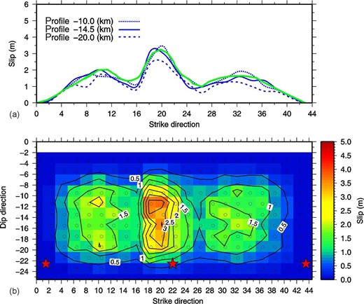
(a) Along-strike maximum slip function SMAX(l) (green curve), as plotted by Pino et al. (2000) for M2. Three different profiles obtained by cutting the slip map shown in panel (b) at the listed depths measured along dip. The slip map represents one of the five realizations generated for M2. The red stars indicate the three tested positions for the nucleation point and the zero depth corresponds to the Earth surface.
For each investigated fault geometry, we generated five different maps of slip (an example for M2 is shown in the bottom panel of Fig. 2). As reported by Cultrera et al. (2010), the value of the ground-shaking level is strongly affected by the relative position of nucleation point and slip patches with respect to the observation point; thus, we also tested three different positions for the nucleation point: one located at the southern edge of the fault plane, one in the middle and one at the northern edge, all at 1.5 km from the bottom of the fault. We tested several rupture velocities, in the subsonic range 1.8–3.0 km s−1, with 0.2 km s−1 step, and rise-time τ in the interval 1.4–1.8 s, with steps of 0.1 s, considering that a suitable value for a M = 7 earthquake is τ = 1.6 s (Sato et al.1989). Overall, for each fault model, we developed 525 source realizations.
We evaluated the PGAs on the simulated accelerograms bandpass filtered in the range 0.01–8.0 Hz and the PGVs from the same accelerograms, integrated and filtered in the range 0.01–2.0 Hz, which is well suited for the specific problem, allowing to take into account for the main effects of both source and propagation.
Then, we modified these values to include site effects. Since no detailed geological information is available for all the selected sites, we used the appropriate VS30 value (shear wave velocity in the upper 30 m) for each site (Michelini et al.2008) and, based on the Borcherdt (1994) approach, we obtained the corrective coefficient for PGA and PGV. Simulated PGAs and PGVs modified by site effects were finally converted in macroseismic intensity MCS by using the empirical relations derived by Faenza & Michelini (2010).
As a first qualitative check of our choice for crustal velocity model and source parameters, we compared the results of all the simulations in terms of PGAs and PGVs with the GMPEs proposed by Boore & Atkinson [2008 (Fig. 3)], computed by using the Joyner-and-Boore (RJB) source-to-site distance metric (i.e. the minimum distance from the surface fault projection; Joyner & Boore 1981). Overall, the simulated data follow a trend very consistent with that predicted by the GMPE. This is even more evident when considering the mean value and the standard deviation of all the data (Fig. 3). However, a larger scatter compared to the ±σ curves (being σ the standard error of the selected GMPE) is displayed as a result of the effect of the different selected kinematic parameters.
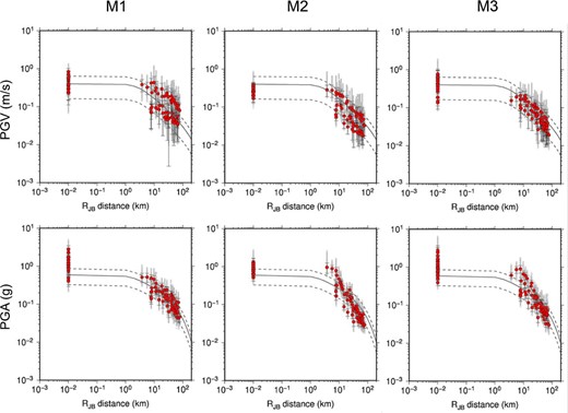
Comparison between synthetics with predicted PGA (bottom) and PGV (top), as a function of RJB distance. The predictions have been obtained by using the GMPEs proposed by Boore & Atkinson (2008). Left panels refer to M1, central panels to M2 and right panels to M3. In each panel, grey dots correspond to the values obtained at the 100 sites for the 525 source realizations; red dots and error bars indicate their average value and standard error, respectively; the continuous line corresponds to the mean value of the GMPE, while the dashed lines correspond to ±σ.
3.3 Misfit evaluation, best model and resolution
Table 3 reports the results for both IPGA and IPGV, in terms of best fitting parameters for each model. For all the models the best rise-time value is 1.4 s, which represents the lower end of the tested range. This is not surprising, since the use of a boxcar source time function corresponds to a low-pass filter of the resulting seismograms. However, the relatively high frequencies required to match the observed macroseismic field push the rise-time towards very low values—well below what would be realistic for a magnitude 7 event (1.6 s; see above)—mapping into rise-time effects what is actually due to propagation or to more complex slip distributions. Based on these considerations, and given the well known trade-off between the rise-time and the rupture velocity (e.g. Emolo et al.2008), we constrained the rise-time to realistic values, allowing only for reasonable variations, without exploring lower values. The rupture velocities providing better fit are always larger than 2.6 km s−1. Moreover, except for IPGA relative to M2 and M3, the best fitting nucleation point position is always located at the southern end of the fault. The last column in Table 3 indicates that among the tested faults, M2 is less adequate to reproduce the observed macroseismic field. The associated misfit values are about 50 per cent larger than what results for the other models. On the other hand, M1 and M3 scores similarly for IPGV, while the former gives a significantly lower value for IPGA. Incidentally, we note the lowest misfit for M1 and M3 result from the same slip map, while M2 is associated with two different maps for IPGA and IPGV, respectively. Overall, according to what stated above, we consider M1 as our best model.
Best model parameters resulting from misfit analysis, for the three tested models and for both PGA and PGV.
| Model | VR (km s−1) | τ (s) | NP | MS | Misfit | |
|---|---|---|---|---|---|---|
| IPGA | 2.8 | 1.4 | S | 1 | 1.412E-4 | |
| M1 | ||||||
| IPGV | 2.8 | 1.4 | S | 1 | 1.437E-4 | |
| IPGA | 3.0 | 1.4 | C | 3 | 1.839E-4 | |
| M2 | ||||||
| IPGV | 3.0 | 1.4 | S | 2 | 2.097E-4 | |
| IPGA | 2.6 | 1.4 | C | 1 | 1.618E-4 | |
| M3 | ||||||
| IPGV | 3.0 | 1.4 | S | 1 | 1.433E-4 |
NP = nucleation point position; southern (S), centre (C)
MS = map slip index. MS indentifies the best slip map, among the 5 generated randomly
For this model, we evaluated the dependence on the parametrization. To this aim, we used an approach similar to seismic hazard deaggregation, in which, during the computation, the contribution of each model to the hazard is saved to build a joint a-posteriori probability density function (Bazzurro & Cornell 1999; Convertito et al.2009). For both IPGA and IPGV, we plotted a binned distribution of all the misfit values (Figs 4a and b) and extracted the model parameters that contribute to the bin with the smallest, the modal and the largest value, respectively (Figs 4c–l). The two distributions display a different shape, with a comparable minimum value but a higher dispersion for IPGV. This effect reflects the higher capability of PGV to discriminate model parameters, with respect to IPGA. In fact, given the relative position of source and sites investigated in this study, the misfit associated to PGA appears to be less affected by the source kinematic details, once the gross position of the major slip patches is defined. As for the other parameters, PGA and PGV are weakly sensitive to the details of the slip distribution (Figs 4e and i), while only few or even a single value contribute to the lowest misfit values for nucleation point position, rupture velocity and rise-time. In particular, for both IPGA and IPGV, all the lowest misfit values are associated with the southern nucleation point, while two pairs of close values for rise-time (1.4 and 1.5 s; Figs 4f and l) and rupture velocity (2.6 and 2.8 km s−1; Figs 4d and h), respectively, provides higher contributions.
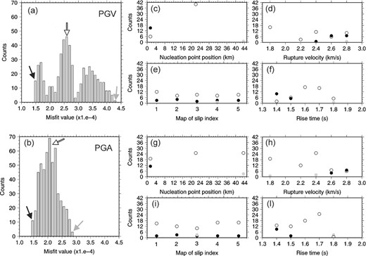
Misfit analysis for the best model M1. The figure shows the dependence of the results on the selected parametrization. Panels (a) and (b) display—respectively for PGV and PGA—the final misfit distribution for IPGV and IPGA, for each set of source parameters. In both panels, black arrow indicates the bin corresponding to the lowest misfit values, thus corresponding to the best performing models; white and grey arrows indicate the bin containing misfit values for modal and worst models, respectively. Plots in (c)–(f) refer to PGV results. The four panels display—respectively, for the indicated source parameters—the values contributing to the lowest misfit bin (black dots), those contributing to the modal bin (white dots), and the ones contributing to the highest misfit values (grey dots). Plots in (g), (h), (i) and (l) show the same for PGA. In panels (c) and (g), the zero distance corresponds to the southern end of the fault.
4 DISCUSSION AND CONCLUSIONS
Fig. 5 shows the maps of PGV and PGA for our preferred model M1. The simulated ground-motion fields display a clear evidence of NW directivity effect, as a result of the southern location of the nucleation point and the consequent northward rupture propagation with updip component. This is in accordance with the results obtained by Pino et al. (2000) and with the modern epicentral location estimated by Michelini et al. (2005). Moreover, we observe that the relative position of the sites with respect to the fault (hangingwall versus footwall effect; e.g. Abrahamson & Somerville 1996; Oglesby et al.1998) and their proximity to the area of maximum slip determine the PGA field pattern, which is affected also by the updip component of the rupture propagation.
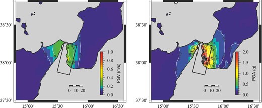
Peak-ground velocity (left) and peak-ground acceleration (right) maps relative to the best-fit model M1. The black rectangles indicate the surface fault projection of the source model M1.
Data and simulated intensity fields are displayed in Fig. 6, together with a map of interpolated data and pointwise representations at the 100 selected sites. Except for a very few points, the computed intensities are all within 1 unit from the observed data. For both IPGA and IPGV, the differences rapidly decrease with distance from the fault, tending to zero at a large number of points, with increasing distance from the source, independently on the azimuth. This indicates that the adopted modelling technique properly accounts for the general attenuation of the intensity with distance, well reproducing the areal distribution of the observed data. As for the kinematic source parameters, the low discrepancy between observed and calculated intensities at sites with RJB = 0 (i.e. located on the surface projection of the fault) confirms the reliability of the adopted parametrization. In fact, at such short distances, the details of the source dominate the high-frequency content of the ground motion, which is generally difficult to be modelled. On the other hand, albeit very large, the PGA (1.0–1.5g; g = gravity acceleration) and PGV (0.5–1.0 m s−1) values predicted at very close distances are still not large enough to reproduce the observed IMAX XI intensity level. This result is likely due to the relationships used to convert the peak-ground motion parameters to intensity and to our modelling of the site effects. As reported above, we used the empirical relation proposed by Faenza & Michelini (2010)—the most recent and robust one for Italy—that was retrieved from intensity data IMCS ≤ 8. Thus, the interpretation of the results for larger values might be biased by its extrapolation. Incidentally, we note that with respect to the one used here, other relations retrieved for different regions (i.e. California; Wald et al.1999) would give higher intensities for large PGA and PGV, but would significantly underestimate the lower intensities (Faenza & Michelini 2010). Concerning the site effects, we are aware that the VS30 and the associated amplification coefficients are just a first-order proxy. However, more realistic modelling would require the knowledge of site transfer functions, at all the tested sites, which are not presently available.
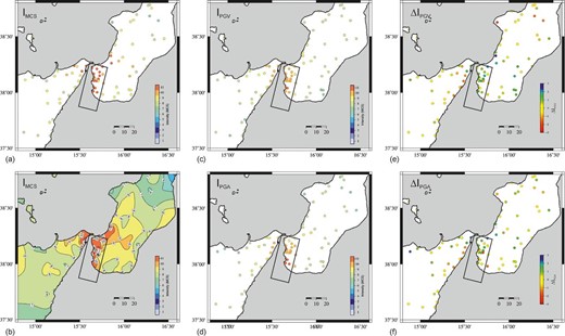
Observed and simulated data: (a) original macroseismic intensities; (b) interpolated original macroseismic intensities; (c) intensities obtained from the simulated PGV relative to the best model M1; (d) same as (c), for PGA; (e) difference between original macroseismic intensities and those obtained from the simulated PGV relative to the best model M1; (f) same as (e), for PGA. In each panel, the black rectangle represents the surface fault projection for M1.
Based on the misfit analysis, we conclude that the modelling of macroseismic data for the 1908 Messina Straits earthquake through simulated PGA allows the discrimination of the best fault location among those analysed. We ascribe this result to the high sensitivity of PGA, as ‘seen’ in proximity of the source, to the fault location and geometry, and to the slip distribution. This confirms the conclusions driven by Imperatori & Mai (2012), who demonstrated that the ground motion is highly sensitive to the source characteristics, at short and intermediate wavelengths, as is the case for acceleration. It is worth to recall here that we adopted the same slip map for all the tested fault models, in practice reducing the number of free parameters. However, as stated above, the use of the original dislocation for M3 would have given a definitely worst match of the observed data, due to the lack of short wavelength details in that model.
Unlike synthetic intensities obtained from computed PGA, PGV-based simulated intensities do not discriminate between M1 and M3, despite the notable difference in their location and dip orientation. This result derives from the strong dependence of the PGV field on the rupture directivity, which, for the 1908 earthquake, was prevalently northward, that is, roughly parallel to the fault strike for both models. As a consequence, the resulting macroseismic field is scarcely affected by the fault dip, making the two models almost indistinguishable. On the other hand, although M1 and M2 display minor differences, they produce very different misfits, confirming that the rupture propagation played a crucial role in the development of the intensity field, above the influence of other source parameters. However, we note that the peculiar distribution of the observation sites might have contributed to the above results.
The above discussion evidences the complementary information provided separately by PGA and PGV. Therefore, as a general conclusion, we consider that the joint analysis of both PGA- and PGV-based simulations is essential to discriminate among different source models, when investigating macroseismic data. Moreover, we demonstrated that direct modelling of intensity data allows constraining source characteristics of large earthquakes such as rise-time and rupture velocity, usually retrieved by analysing instrumental data. This shows that macroseismic data include additional information on earthquake source kinematics, with respect to what already shown by previous studies (e.g. Gasperini et al.1999; Pettenati & Sirovich 2007).
The results described in the present study further confirm the considerable amount of information carried by macroseismic data, which are fundamental for investigating the source of historical earthquakes. This, in turn, has great importance for the definition of the seismic input in the context of hazard analyses and risk mitigation.
We thank Antonio Emolo for discussion and a careful reading of a first manuscript version. We also thank Josep Battló, the Editor Ingo Grevemeyer and an anonymous reviewer for their constructive criticisms. The figures were prepared with Generic Mapping Tools (Wessel & Smith 1991).
