


Abstract
We use simulations of Milky Way-sized dark matter haloes from the Aquarius Project to investigate the orbits of substructure haloes likely, according to a semi-analytic galaxy formation model, to host luminous satellites. These tend to populate the most massive subhaloes and are on more radial orbits than the majority of subhaloes found within the halo virial radius. One reason for this (mild) kinematic bias is that many low-mass subhaloes have apocentres that exceed the virial radius of the host; they are thus excluded from subhalo samples identified within the virial boundary, reducing the number of subhaloes on radial orbits. Two other factors contributing to the difference in orbital shape between dark and luminous subhaloes are their dynamical evolution after infall, which affects more markedly low-mass (dark) subhaloes, and a weak dependence of ellipticity on the redshift of first infall. The ellipticity distribution of luminous satellites exhibits little halo-to-halo scatter, and it may therefore be compared fruitfully with that of Milky Way satellites. Since the latter depends sensitively on the total mass of the Milky Way we can use the predicted distribution of satellite ellipticities to place constraints on this important parameter. Using the latest estimates of position and velocity of dwarfs compiled from the literature, we find that the most likely Milky Way mass lies in the range 6 × 10¹¹ M⊙ < M200 < 3.1 × 10¹² M⊙, with a best-fitting value of M200 = 1.1 × 10¹² M⊙. This value is consistent with Milky Way mass estimates based on dynamical tracers or the timing argument.
INTRODUCTION
Satellite galaxies have long been used as kinematic tracers of the gravitational potential of the Milky Way (MW) halo (e.g. Hartwick & Sargent 1978; Lynden-Bell, Cannon & Godwin 1983; Zaritsky et al. 1989; Kulessa & Lynden-Bell 1992; Kochanek 1996; Wilkinson & Evans 1999; Battaglia et al. 2005; Sales et al. 2007a; Boylan-Kolchin et al. 2013). The usefulness of this technique, however, has been traditionally limited by the relatively small number of satellites known, by uncertainties in their estimated distances, and by the availability of a single component of the orbital velocity, along the line of sight. This state of affairs, however, is starting to change.
Over the last decade, surveys like the Sloan Digital Sky Survey (SDSS) have mapped large areas of the sky, an effort that has led to the discovery of a number of very faint satellite galaxies (the ‘ultrafaint’ dwarf spheroidal companions of the MW) whose star formation history, chemical evolution, mass, distance and velocity have now been estimated through deep follow-up observations (e.g. Willman et al. 2005; Zucker et al. 2006a,b; Belokurov et al. 2007; Irwin et al. 2007; Walsh, Jerjen & Willman 2007; Kirby et al. 2008; Martin, de Jong & Rix 2008; Adén et al. 2009; Norris et al. 2010; Wolf et al. 2010; Simon et al. 2011; Brown et al. 2012). Distance estimates have also improved, to the point that the distances to most satellites are now known to better than ∼10 per cent from measurements of resolved stellar populations. Further, the superior angular resolution of the Hubble Space Telescope (HST) has enabled proper motion estimates for nearby dwarfs from images with a time baseline of just a few years (e.g. Piatek et al. 2002), and modern adaptive optics systems promise to reach comparable angular resolution from the ground (e.g. Rigaut et al. 2012). Finally, in the near future, a great leap forward is expected from the Global Astrometry Interferometer for Astrophysics (Gaia) satellite (e.g. Lindegren & Perryman 1996). This mission is expected to measure the proper motions of the MW dwarf spheroidal system to an accuracy of a few to tens of km s−1, depending on the satellite's properties (Wilkinson & Evans 1999).
Accurate proper motions, radial velocities, positions and distances can be used to compute satellite orbits after assuming a mass profile for the Galaxy. The shapes of these orbits are expected to contain information about the circumstances of the accretion of individual satellites, as well as about the evolution of the potential well of the Galaxy over time. Decoding such information, however, is not straightforward, and is best attempted by contrasting observations with realistic simulations that resolve in detail the dynamical evolution of the potential sites of dwarf galaxy formation.
Although there are in the literature a number of studies of the kinematics of satellite systems and their relation to the haloes they inhabit (e.g. Tormen 1997; Ghigna et al. 1998; Tormen, Diaferio & Syer 1998; van den Bosch et al. 1999; Balogh, Navarro & Morris 2000; Taffoni et al. 2003; Gill et al. 2004; Kravtsov, Gnedin & Klypin 2004; Gill, Knebe & Gibson 2005; Diemand, Kuhlen & Madau 2007; Sales et al. 2007a; Ludlow et al. 2009), most have dealt primarily with the orbits of substructure haloes (referred to hereafter as subhaloes) in general. Luminous satellites inhabit a small fraction of subhaloes, and their orbits might therefore very well be substantially biased relative to those of typical subhaloes. Making progress demands not only simulations with numerical resolution high enough to resolve all potential sites of luminous satellite formation but also a convincing way of pinpointing the few subhaloes where those satellites actually form.
A number of simulations that satisfy the numerical resolution requirement have been recently completed, notably the six MW-sized haloes of the Aquarius Project (Springel et al. 2008), as well as the Via Lactea II halo (Diemand et al. 2008), and its higher resolution version GHALO (Stadel et al. 2009). In this study, we combine the Aquarius Project haloes with the semi-analytical model of Starkenburg et al. (2013) to identify satellites with luminosities down to the ‘ultrafaint’ regime. We study the orbital distribution of these satellites, and explore its dependence on satellite properties such as stellar mass and accretion time. Our analysis yields predictions that should prove useful in the near future, when Gaia delivers accurate 6D phase space information for many MW satellites. We describe here a possible application, making use of published proper motions, positions and radial velocities of the most luminous MW satellites to constrain the mass of the MW halo.
The plan of this paper is as follows. In Section 2, we describe the simulated satellite sample we use, together with a brief discussion of the numerical simulations and of the semi-analytic galaxy formation model adopted. We describe the analysis techniques used to compute orbital properties for satellites and subhaloes and present their orbital ellipticity distributions in Section 3. We investigate in the same section the origin of their differences before, finally, in Section 4, comparing the orbits of simulated dwarf galaxies to those of MW dwarfs in order to discuss the constraints they imply on the total virial mass of the MW. We summarize our main conclusions in Section 5.
SIMULATED SATELLITES
The N-body Simulations
The Aquarius Project consists of a suite of six high-resolution dark matter-only simulations of haloes with virial mass1M200 in the range (0.8–1.8) × 1012 M⊙. We use the level-2 resolution runs of all six Aquarius haloes (named Aq-A through Aq-F), resolved with several hundred million particles each (see Springel et al. 2008, for details). The numerical resolution of the level-2 Aquarius haloes allows us to track dark matter haloes with masses as small as 105 M⊙, which we identify and track using the groupfinder subfind (Springel et al. 2005). This algorithm recursively identifies all self-bound substructures with at least 20 particles present within a set of haloes first identified using a standard friends-of-friends technique (Davis et al. 1985).
All simulations assume a ‘standard’ Λ cold dark matter (ΛCDM) cosmogony, with the same parameters as the Millennium Simulation (Springel et al. 2005): ΩM = 0.25, ΩΛ = 0.75, n = 1, h = 0.73 and σ8 = 0.9. Although these parameters are now out of favour considering the recently published results from the Planck satellite (Planck Collaboration 2013), we expect them to have little effect on the detailed non-linear structure and substructure of dark matter haloes which concern us here (see, e.g. Wang et al. 2008; Boylan-Kolchin et al. 2010; Guo et al. 2013).
The semi-analytic model
A semi-analytic model of galaxy formation is grafted on to the evolving collection of subfind haloes and subhaloes linked as a function of time by a merger tree (Baugh 2006; Benson 2010). The particular model implementation we use is described by Starkenburg et al. (2013) and is an extension of earlier work (Kauffmann et al. 1999; Springel et al. 2001; De Lucia, Kauffmann & White 2004; Croton et al. 2006; De Lucia & Blaizot 2007; De Lucia & Helmi 2008; Li et al. 2009; Li, De Lucia & Helmi 2010). The main ingredients for the model are analytic prescriptions for gas-cooling, re-ionization, star formation and stellar feedback. Interactions of a satellite galaxy with its host are included in the form of stellar stripping and tidal disruption as well as ram-pressure stripping, an effect that leads to the removal of the hot gas reservoir from satellites after infall.
As discussed by Starkenburg et al. (2013), the simulated satellite luminosity function of Aquarius haloes is consistent with that of the MW. Luminous satellites populate a minority of the subhalo population, preferentially the high-mass end. Indeed, by number, most subhaloes have low mass and, according to the model, remain completely ‘dark’ throughout their lifetime.
Satellite sample
The semi-analytic model assigns a stellar mass (or luminosity) to each subhalo at the present time. We classify them as (i) ‘classical’ satellites (i.e. those brighter than MV = −8), (ii) ‘ultrafaint’ satellites (fainter than MV = −8) and (iii) ‘dark’ subhaloes (i.e. those with no stars). We shall hereafter use the term ‘luminous subhaloes’ to refer to classical and ultrafaint satellites combined.
This classification makes reference to the MW, where the ‘classical’ satellite population is expected to be complete within the boundaries of the Galactic halo with the exception perhaps of the ‘zone of avoidance’ created by dust absorption in the Galactic disc. ‘Ultrafaint’ satellites, on the other hand, have only recently been discovered in SDSS data. Their inventory is far from complete and their spatial distribution highly biased to relatively small nearby volumes in the region surveyed by SDSS (Koposov et al. 2008). Because of this, we shall restrict much of the comparison of our models with data on classical satellites.
ANALYSIS AND RESULTS
Satellite masses and radial distribution
Fig. 1 shows the mass distribution of all subhaloes identified at z = 0 within the virial radius, r200, of each of the six Aquarius haloes considered here. Masses are quoted at the time of first infall into the main progenitor of each halo (tinf), and correspond roughly to the maximum virial mass of each subhalo prior to accretion. We also show in Fig. 1 the subhalo masses of the luminous satellites and confirm that, as expected, they tend to populate the most massive subhaloes.
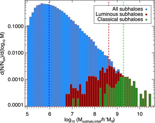
Mass distribution of subhaloes found, at z = 0, within the virial radius, r200, of the level-2 Aquarius A–F haloes. Their (virial) masses are computed at the time of first infall into the main progenitor of the main halo. All subhaloes are shown in blue, luminous satellites in red and classical satellites in green. Vertical dashed lines indicate the median of each group. Luminous satellites populate preferentially the high-mass end of the subhalo mass function. The decline in numbers below ∼106 h−1 M⊙ results from limited numerical resolution. We consider only subhaloes with masses exceeding ∼106 h−1 M⊙ in our subsequent analysis.
Low-mass subhaloes clearly dominate the numbers down to 106 M⊙, where the distribution peaks. The decline in numbers at lower masses results from limited numerical resolution (see Springel et al. 2008, for a detailed discussion). We shall therefore consider for analysis only subhaloes with virial mass exceeding 106 M⊙ at first infall, or haloes with more than ∼100 particles. Combining all six simulations, our full satellite sample consists of 50 874 subhaloes, of which 452 host luminous satellites: 296 ultrafaint and 156 classical dwarfs, respectively.
Fig. 2 shows the radial distribution of the three populations of subhaloes in our model. Luminous satellites are noticeably more centrally concentrated than the majority of subhaloes (e.g. Gao et al. 2004; Starkenburg et al. 2013), a bias that might affect the comparison between the orbital properties of luminous and dark subhaloes. Another noticeable difference between the luminous and non-luminous subhalo population is the distribution of their infall times, tinf: as shown in Fig. 3, the luminous subhaloes tend to fall in earlier.
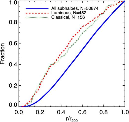
Fraction of enclosed subhaloes as a function of radius for level-2 Aquarius haloes A through F. All subhaloes are shown as a blue solid line, the subset of luminous satellites as a red dashed line and only the classical as a green dotted line.
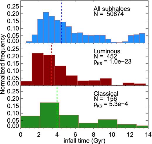
Distribution of first-infall cosmic times (where zero corresponds to the big bang) for satellites identified within the virial radius of the main halo at z = 0. Medians are indicated by vertical dashed lines. The normalization of the frequency is chosen such that the area under each histogram equals unity. Luminous (i.e. ultrafaint and classical) satellites enter the most massive progenitor of the main halo earlier than the average subhalo. N indicates the number of subhaloes in each grouping. KS tests indicate the probability that the luminous or classical samples are drawn from the same parent population as all subhaloes.
Orbital ellipticity distributions
The ellipticity distributions of the three subhalo populations at z = 0 are shown in Fig. 4. The orbits of luminous satellites are clearly more radial than those of the subhalo population as a whole, which is dominated by the numerous low-mass, ‘dark’ systems. Half of all subhaloes are on orbits with e < 0.59, but the median e is significantly larger for luminous systems: 0.68 for all luminous and 0.65 for classical satellites. As indicated by a Kolmogorov–Smirnov (KS) test, the distributions are very significantly different indeed. (The probability that the e-distribution of each satellite grouping is drawn from the same parent distribution as all subhaloes is listed in the middle and bottom panels.) This result is in qualitative agreement with pioneering work from Tormen (1997) who found that within simulated cluster environments more massive satellites move along more eccentric orbits than lower mass satellites.
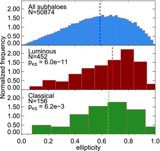
As in Fig. 3, but for the ellipticity distributions of all subhaloes (top), all luminous (middle) and just the classical dwarfs (bottom), measured at z = 0. Medians are indicated by vertical dashed lines. KS tests indicate the probability that the observed luminous and classical satellite ellipticities are drawn from the same parent population as that of all subhaloes.
Classical satellites are on slightly less radial orbits than ultrafaints (as is reflected in the higher median e for all luminous subhaloes, compared to just the classical satellite subset), but the difference between the two has lower significance; a KS test yields a p-value of 0.65.
We note that our modelling neglects the effect of baryons and, in particular, of the potential modifications that the presence of a massive stellar disc may have on the subhalo mass function and their orbits. A recent study by D'Onghia et al. (2010), for example, shows that disc shocking may be able to destroy preferentially low-mass subhalos on plunging orbits. This would presumably skew their ellipticity distribution to less radial orbits and would enhance the differences noted above between the ellipticity distributions of ‘dark’ subhaloes and ‘luminous’ satellites.
Radial selection biases and dynamical evolution
What is the origin of the systematic differences in the orbital shapes of luminous and dark subhaloes?
A clue is provided by the distribution of infall times of all subhaloes. As seen in the top panel of Fig. 3, a notable feature is that there is a well-defined dip in the number of satellites with tinf of the order of ∼11 Gyr, followed by a sharp upturn a couple of Gyr later. We have verified that the dip is actually present in all Aquarius haloes taken individually, and does not reflect a particular event in the accretion history of individual haloes.
Rather, the dip may be traced to the fact that many subhaloes accreted at tinf ∼ 11 Gyr are found temporarily outside the virial boundary of the halo at z = 0. Indeed, the radial period of an object released at rest from the virial radius is roughly ∼3 Gyr; most systems accreted at tinf ∼ 11 Gyr have apocentric radii that exceed r200, and the majority of them are today therefore beyond the formal virial boundary of the halo. As discussed in detail by Ludlow et al. (2009) (see also Balogh et al. 2000; Mamon et al. 2004; Gill et al. 2005; Diemand et al. 2007; Ludlow et al. 2009; Wang, Mo & Jing 2009), subhaloes identified within the virial radius represent a rather incomplete census of the substructure physically related to a halo: many ‘associated2’ subhaloes are found outside the formal virial radius of a halo at any given time. The effect is mass dependent: associated subhaloes outside r200 tend to be preferentially low mass.
We show this explicitly in Fig. 5, where we compare the apocentric radii of all associated subhaloes with those of luminous ones. Selecting systems within r200 includes more than 80 per cent of all luminous associated satellites, but leaves out nearly half of the less massive, dark subhaloes. This introduces a substantial bias in the apocentric radii of the latter, selecting preferentially systems with smaller apocentres. The effect on the orbital ellipticity distribution is to favour systems with less radial orbits.
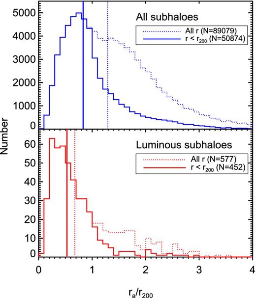
Distribution of apocentric radii for all subhaloes and luminous subhaloes (top and bottom panels, respectively). Solid lines correspond to subhaloes found within r200 at z = 0; dotted lines to all ‘associated’ subhaloes. Note that few (∼20 per cent) luminous subhaloes are found outside the virial radius; on the other hand, selecting only systems within the virial radius excludes nearly half of all (mostly low-mass) associated subhaloes.
This may be seen in Fig. 6, where we compare the ellipticity distributions of various samples of luminous and dark subhaloes. The top two panels show that the dark and luminous subhalo ellipticity distributions become more similar when considering all associated subhaloes rather than selecting only those within r200. The radial selection bias, however, is not enough to explain the systematic difference between the two populations, as shown by the low probability of a KS test (see legends in each panel of Fig. 6).
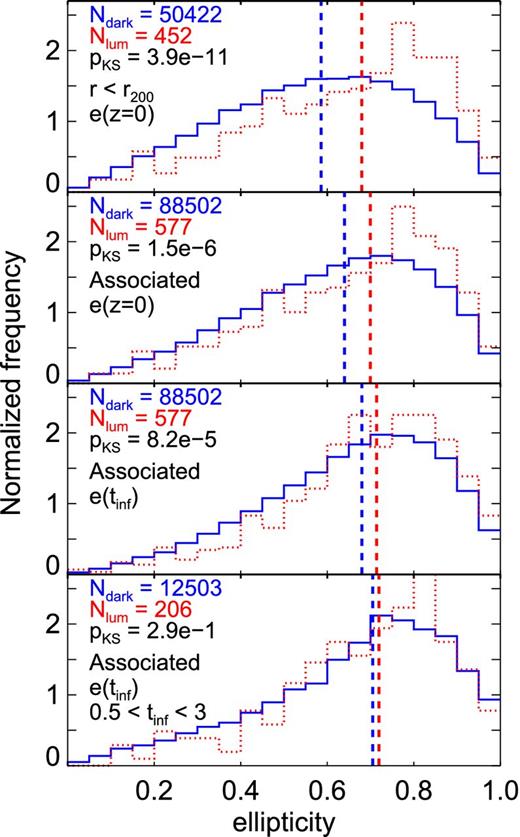
Ellipticity distributions of luminous and non-luminous subhaloes (red dotted and blue solid lines, respectively). Medians are indicated by vertical dashed lines. The listed p-values in each panel correspond to the KS test between the luminous and non-luminous subhalo distributions shown in that panel. The normalization is chosen such that the area under each curve is unity. Top panel: only subhaloes with r < r200 are considered, their ellipticity distributions are measured at z = 0. Second panel: same as in the top panel, but including all ‘associated’ subhaloes. Third panel: same as in the second panel, except that the ellipticity distribution is measured at the time of first infall. Bottom panel: same as in the third panel, but with the subhalo sample restricted to those subhaloes that have fallen into the main halo between 0.5 and 3 Gyr.
The remaining difference is due partly to the fact that the orbits of dark and luminous subhaloes evolve differently after being accreted into the main halo. This is shown in the third panel of Fig. 6, where ellipticities measured at the time of first infall are compared. Although still significantly different, ellipticities of associated dark and luminous subhaloes are much closer at infall than at z = 0.
The top three panels of Fig. 6 also indicate that it is mainly the ellipticities of low-mass (dark) subhaloes that change appreciably after infall: their orbits tend to become less radial with time, something that is not seen in the luminous satellites. Possible scenarios for this ‘circularization’ of low-mass subhaloes include the tidal dissolution of the groups to which they belong at accretion, but also perturbations by massive subhaloes they encounter on their orbits within the host halo (e.g. Tormen et al. 1998; Taffoni et al. 2003). We have explicitly checked that this conclusion is not the result of limited numerical resolution: we obtain similar results even if we raise the minimum subhalo mass considered in our sample from 106 to 107 M⊙, or even 108 M⊙.
Finally, when comparing the ellipticities at infall, the difference between dark and luminous subhaloes vanishes when considering systems that were accreted in the same infall time window (bottom panel of Fig. 6). This is because satellites that fall in early tend to be on slightly more radial orbits, as suggested by Wetzel (2011). Selecting systems with similar infall times removes this dependence and brings the ellipticity distribution of dark and luminous subhaloes into agreement.
We conclude that the orbital difference between dark and luminous subhaloes shown in Fig. 4 is due to the combined effects of mass-dependent dynamical evolution after infall, a dependence of ellipticity with infall time, and by the selection bias introduced by considering only systems within the virial radius.
APPLICATION TO THE MILKY WAY
One main conclusion of the previous analysis is that cosmological simulations make well-defined predictions for the ellipticity distribution of satellite galaxies. These predictions cannot be compared directly to observations because the only available data are instantaneous positions and velocities for those satellites with distance, radial velocity and proper motion estimates. A literature search yields such data for 9 of the 13 MW satellites brighter than MV = −8. These positions and velocities may be used to estimate orbital ellipticities after assuming a mass profile for the Galaxy. This allows us to place constraints on the total mass of the Galaxy by requiring that the ellipticity distribution matches that of simulated luminous satellites. We pursue this idea in Section 4.2, after presenting the observational data set we use in Section 4.1.
MW satellite ellipticities
We summarize in Table 1 the MW satellite literature data used in our analysis. When several different estimates are available we have adopted values from the recent compilation of McConnachie (2012). We have exclusively adopted proper motion estimates from HST data.
Data for MW satellites taken from the literature. Proper motions are given in equatorial coordinates; distances and velocities have been converted to a Galactocentric frame.
| μα | μδ | |$D_{\text{MW}}$| | Vr | Vt | |||
|---|---|---|---|---|---|---|---|
| Galaxy | MV | (mas/century) | (mas/century) | (kpc) | (km s−1) | (km s−1) | References |
| Ursa Minor | −8.8 | −50.0 ± 17.0 | 22.0 ± 16.0 | 78 ± 3 | −58.5 ± 6.4 | 157.8 ± 54.8 | 0,1,2 |
| Carina | −9.1 | 22.0 ± 9.0 | 15.0 ± 9.0 | 107 ± 6 | −4.8 ± 3.9 | 94.9 ± 40.1 | 3,4,5 |
| Sculptor | −11.1 | 9.0 ± 13.0 | 2.0 ± 13.0 | 86 ± 6 | 78.0 ± 5.1 | 243.8 ± 52.9 | 6,7,5 |
| Fornax | −13.4 | 47.6 ± 4.6 | −36.0 ± 4.1 | 149 ± 12 | −38.8 ± 1.9 | 185.9 ± 45.3 | 8,4,5 |
| Leo II | −9.8 | 10.4 ± 11.3 | −3.3 ± 11.5 | 236 ± 14 | 14.9 ± 4.3 | 312.4 ± 118.5 | 9,10,11 |
| Leo I | −12.0 | −11.4 ± 3.0 | −12.6 ± 2.9 | 258 ± 15 | 167.6 ± 1.6 | 106.6 ± 34.0 | 12,13,14 |
| SMC | −16.8 | 75.4 ± 6.1 | −125.2 ± 5.8 | 61 ± 4 | −9.8 ± 2.8 | 256.3 ± 32.7 | 15,16,17 |
| LMC | −18.1 | 195.6 ± 3.6 | 43.5 ± 3.6 | 50 ± 2 | 67.2 ± 4.0 | 342.5 ± 20.9 | 15,18,19 |
| Sagittarius dSph | −13.5 | −275.0 ± 20.0 | −165.0 ± 22.0 | 18 ± 2 | 140.9 ± 3.9 | 274.2 ± 32.7 | 20,21,22 |
References: 0 = Piatek et al. (2005), 1 = Carrera et al. (2002), 2 = Walker et al. (2009b), 3 = Piatek et al. (2003), 4 = Pietrzyński et al. (2009), 5 = Walker, Mateo & Olszewski (2009a), 6 = Piatek et al. (2006), 7 = Pietrzyński et al. (2008), 8 = Piatek et al. (2007), 9 = Lépine et al. (2011), 10 = Bellazzini, Gennari & Ferraro (2005), 11 = Walker et al. (2007), 12 = Sohn et al. (2013), 13 = Bellazzini et al. (2004), 14 = Mateo, Olszewski & Walker (2008), 15 = Piatek, Pryor & Olszewski (2008), 16 = Udalski et al. (1999), 17 = Harris & Zaritsky (2006), 18 = Clementini et al. (2003), 19 = van der Marel et al. (2002), 20 = Pryor, Piatek & Olszewski (2010), 21 = Monaco et al. (2004), 22 = Ibata, Gilmore & Irwin (1994).
In order to facilitate comparison between observation and simulation, we have transformed all values to a Cartesian Galactocentric coordinate system, with the x-axis pointing in the direction from the Sun to the Galactic Centre, y-axis pointing in the direction of the Sun's orbit and z-axis pointing towards the Galactic North Pole. We assume a velocity of V0 = 239 ± 5 km s−1 for the clockwise circular velocity of the local standard of rest (LSR; McMillan 2011); R0 = 8.29 ± 0.16 kpc for the distance from the Sun to the Galactic Centre, as well as (U, V, W) = (11.10 ± 1.23, 12.24 ± 2.05, 7.25 ± 0.62) km s−1 for the Sun's peculiar velocity with respect to the LSR from Schönrich, Binney & Dehnen (2010).
We compute ellipticities for all nine satellites assuming that the mass profile of the Galaxy may be approximated by an NFW halo with concentration given by the mass–concentration relation of Neto et al. (2007). We have explicitly verified that the results we quote are insensitive to the exact value of the concentration: for example, varying c between 8 and 17 for a halo of virial mass M200 = 1.1 × 10¹² M⊙ leads to an average change in the ellipticity of 0.05 over all nine satellites. This variation is much smaller than the uncertainty implied by the relatively poor accuracy of the proper motion estimates.
The coloured lines in Fig. 7 show how the ellipticities estimated for each MW satellite change as the assumed mass of the MW is varied from M200 = 5 × 10¹¹ to 5 × 10¹² M⊙. As anticipated in Section 1, the ellipticity of a satellite depends sensitively on the mass of the Galaxy. For example, if a satellite's radial velocity is much smaller than its tangential velocity, then it must be either close to apocentre or pericentre. If near pericentre, increasing the Galaxy mass will decrease its apocentric radius and make the orbital ellipticity decrease. If near apocentre, then the pericentre decreases as the mass increases, resulting in a more elliptical orbit instead.3
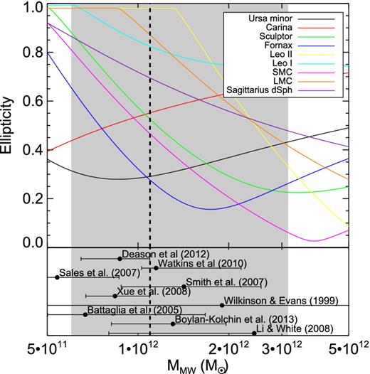
The ellipticity of orbits computed for all MW satellites with proper motion measurements (given in Table 1) as a function of the assumed MW virial mass. The vertical dashed line gives the most likely MW mass as determined in this work and the grey area the 95 per cent confidence limits. The bottom panel shows MW virial mass estimates from various literature sources, converted to M200 (see the text for details).
We note that a number of previous studies have suggested a possible connection between episodes of star formation history in satellites and pericentric passages during their orbits around the MW (e.g. Mayer et al. 2007; Pasetto et al. 2011; Nichols, Lin & Bland-Hawthorn 2012). The strong dependence of the timing of such episodes on the assumed mass of the MW provides an interesting constraint. It would be particularly interesting, for example, to see if the same MW mass leads to synchronized pericentric passages and star formation episodes for a number of satellites, an issue we plan to address in future work.
The mass of the MW
As Fig. 7 makes clear, in general the lower the total mass the larger the inferred orbital ellipticity of a satellite. For example, the median ellipticity of the nine MW satellites increases from 0.4 to 0.98 as the mass is varied in the range described above. The corresponding cumulative ellipticity distribution for several distinct choices of the MW mass is shown in the top panel of Fig. 8 (coloured lines) and compared with that of classical satellites in Aquarius (thin grey lines for individual haloes and a thick black line for all haloes combined).
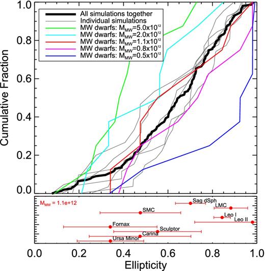
Top panel: cumulative ellipticity distributions of classical satellites from Aquarius haloes. Results for individual haloes are shown in thin grey; that for all six haloes combined is shown in thick black. Coloured lines show the ellipticity distribution of the nine classical dwarfs for which data are available, assuming different values for the virial mass of the MW (see legends). Bottom panel: ellipticities estimated for each MW dwarf (arbitrarily offset in y for clarity) assuming the best match halo virial mass for the MW from this work, M200 = 1.1 × 10¹² M⊙. 1σ error bars are given.
Note that the ellipticity distributions of individual Aquarius haloes are very similar despite large differences in their accretion history and the fact that they span a sizeable mass range (Springel et al. 2008). Even Aq-F, which underwent a recent major merger and is thus an unlikely host for the MW, is indistinguishable from the rest. We caution, however, that our analysis is based on only six haloes, which precludes a proper statistical study of the halo-to-halo scatter. Future simulations should be able to clarify this, as well as the possible dependence of satellite properties as a function of halo mass and environment. Encouragingly, our conclusion agrees with the earlier work by Gill et al. (2004), who analyse eight simulations chosen to sample a variety of formation histories, ages and triaxialities, and report a striking similarity in the ellipticity distribution of their satellite systems. Furthermore, Wetzel (2011) find that the ellipticity distribution of satellites at z = 0 is independent of host halo mass in systems less massive than ∼4 × 10¹² M⊙, a range that comfortably includes most current estimates of the MW virial mass.
We conclude that comparing MW satellite ellipticities with the simulation predictions offers a viable alternative method for estimating the MW mass. The best match (as measured by the maximum value of the KS probability obtained when comparing the nine MW satellite ellipticities to all six Aquarius haloes) is obtained for M200 = 1.1 × 10¹² M⊙. Values less than 6 × 10¹¹ M⊙ or larger than 3.1 × 10¹² M⊙ are disfavoured at better than 95 per cent confidence according to the same test.
The bottom panel of Fig. 8 shows the ellipticities for all satellites for the favoured MW mass including 1σ error bars. Lux, Read & Lake (2010) show that measurements with Gaia's expected accuracy will enable calculations of the last apo- and pericentres of each orbit to an accuracy of ∼14 per cent for a given MW potential, whereas current observational data only allow recovery to ∼40 per cent accuracy. The Gaia data set will thus greatly enhance the accuracy of the MW mass determination using this method.
In Fig. 7, the currently favoured mass range is shown by the black dashed line and grey shaded area. We compare in the same figure our results with independent estimates based on a variety of methods, from the timing argument (Li & White 2008) to the kinematics of halo stars (Battaglia et al. 2005; Smith et al. 2007; Xue et al. 2008; Deason et al. 2012), to virial estimates based on satellite kinematics (Wilkinson & Evans 1999; Battaglia et al. 2005; Sales et al. 2007a; Watkins, Evans & An 2010; Boylan-Kolchin et al. 2013). When other mass definitions were used, the estimates given in these papers have been converted to M200 assuming NFW profiles with concentrations computed from Neto et al. (2007). Some of these values require extrapolating masses measured within smaller radii out to the virial radius. In spite of this, it is striking that all literature values are in reasonable agreement with our determination, lending support to the viability of our method.
The associated satellites of the MW
As discussed in the previous section, a number of satellites associated with the main halo are found today beyond the formal virial boundaries of the halo. Although this applies mostly to low-mass subhaloes, a small fraction (∼20 per cent) of luminous satellites outside r200 at z = 0 have also been associated with the main halo. Can we use their orbits to identify them? This is important because associated satellites are more likely to have experienced tidal and ram-pressure stripping and to have evolved differently from ‘field’ dwarfs.
We explore this idea in Fig. 9, where we compare the Galactocentric radial velocities and distances of ‘classical’ dwarfs in our model and in the vicinity of the MW. The figure includes only Local Group dwarfs that are closer to the MW than they are to the Andromeda galaxy. All Aquarius main haloes have been normalized to M200 = 1.1 × 10¹² M⊙, our best match MW mass as determined in the previous section. Associated model dwarfs are plotted with red triangles and blue crosses denote dwarfs that have never been associated with the main halo.
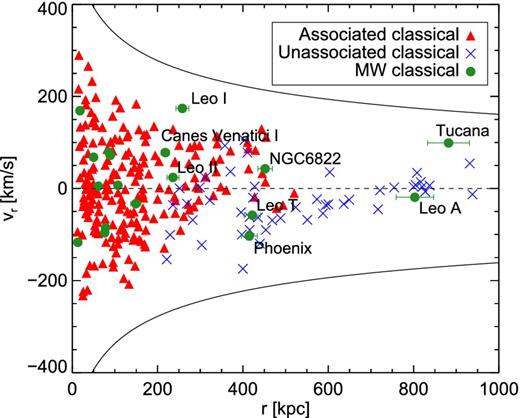
Radial distance of classical subhaloes in the Aquarius simulations versus their radial velocity. All Aquarius subhalo data have been scaled to the best-fitting virial mass of M200 = 1.1 × 10¹² M⊙ as derived in the previous section. Red triangles correspond to the associated classical subhaloes (i.e. subhaloes that have at some time been inside the virial radius of the main halo) whereas blue crosses are classical subhaloes that have never been within the main halo. Overplotted in green filled circles are the classical dwarf galaxies within the Local Group that have the MW as their nearest massive neighbour (i.e. galaxies that are closer to M31 than to the MW are not included). The solid lines show the escape velocity of the MW, computed assuming an NFW halo with concentration equal to 8.52.
Interestingly, most subhaloes located between ∼300 and ∼500 kpc that are moving away from the main galaxy are ‘associated’, whereas those with negative radial velocity tend to be unassociated dwarfs on first infall. Furthermore, beyond ∼600 kpc no classical dwarf has been associated with the main halo.
Some of these conclusions are in apparent conflict with the results obtained by Teyssier, Johnston & Kuhlen (2012), who use associated subhaloes from the Via Lactea II simulation, and report a significant population of associated subhaloes out to 1.5 Mpc from the host halo. One important reason for this apparent conflict is that Teyssier et al. (2012) do not discriminate between subhaloes likely to host a dwarf as bright as a ‘classical’ dSph. Indeed, some associated subhaloes in Aquarius are also found beyond 1 Mpc, but these are exclusively low-mass haloes unlikely, according to our semi-analytical model, to host dwarfs brighter than MV = −8.
We end with a word of caution, however. Our Aquarius main haloes do not have a massive companion and the simulations therefore do not attempt to reproduce the large-scale distribution of matter of the Local Group, where two massive haloes (those surrounding the MW and M31) are about to collide for the first time. The main halo in the Via Lactea II simulation does have a massive neighbour, which results in a much larger turnaround radius for this system when compared to any of the Aquarius systems. The effect of a Local Group environment on the kinematics of outlying dwarfs has not been properly studied yet, but there are indications that it is likely to play an important role in the accretion history of satellite galaxies and in the evolution of neighbouring dwarfs (see, e.g. Benítez-Llambay et al. 2013).
SUMMARY AND CONCLUSIONS
We have combined the semi-analytical modelling of Starkenburg et al. (2013) with the high-resolution simulations of the Aquarius project to investigate the orbits of the satellites of MW-sized haloes in a ΛCDM universe.
We find that the orbital ellipticity distribution of luminous satellites shows little halo-to-halo scatter and is radially biased relative to that of all subhaloes ‘associated’ with the main halo. The bias is relatively mild, considering that luminous satellites populate preferentially massive subhaloes and are more centrally concentrated than the main subhalo population. The bias results from the combination of three main effects: (i) selecting subhalo samples only within the virial radius; (ii) dynamical evolution after infall; and (iii) a weak dependence of ellipticity with infall time.
The first arises because many low-mass subhaloes (which dominate by number but are generally dark) have apocentric radii larger than the virial radius and are thus found outside r200 at any given time. The second likely results from interactions between substructures, which have a more pronounced effect on low-mass subhaloes. Our results therefore urge caution when selecting only subhaloes within the virial radius, since many associated subhaloes (especially low-mass ones) lie at any given time outside the virial radius.
We have compared the ellipticity distribution predicted for luminous satellites with that estimated for nine MW satellites with available 6D phase space data. Since the latter depends sensitively on the total mass assumed for the MW, this comparison allows us to place interesting constraints on the MW mass. We find that the ellipticity distribution of MW satellites is consistent with the predicted one (at 95 per cent confidence) only if the MW virial mass is in the range 6 × 10¹¹–3.1 × 10¹² M⊙. This determination is in agreement with current, independent constraints from other observations, and is subject to improvement as the sample of satellites with proper motion estimates increases and the accuracy of such measurements improves.
The authors are indebted to the Virgo Consortium, which was responsible for designing and running the halo simulations of the Aquarius Project. They are also grateful to Gabriella De Lucia, Amina Helmi and Yang-Shyang Li for their role in developing the semi-analytic model of galaxy formation used in this paper. ES gratefully acknowledges the Canadian Institute for Advanced Research (CIfAR) Global Scholar Academy and the Canadian Institute for Theoretical Astrophysics (CITA) National Fellowship for partial support.
CIFAR Global Scholar and CITA National Fellow.
CIFAR Senior Fellow.
We define all halo ‘virial’ quantities (labelled with a ‘200’ subscript) as those measured within a sphere of mean density 200 times the critical density for closure, ρcrit.
We denote as ‘associated’ all subhaloes that survive to z = 0 and were, at any time during their evolution, within the (evolving) virial radius of the main halo. The number of associated subhaloes nearly doubles the number within the virial radius: we identify 89 079 associated subhaloes in all six level-2 Aquarius haloes.
These comments assume that the satellite remains bound as the Galaxy mass changes. Note that Leo I, Leo II and the Large Magellanic Cloud would be unbound if the MW virial mass was less than 6 × 10¹¹, 1.5 × 10¹² and 8 × 10¹¹ M⊙, respectively.
