


Abstract
Equipartition arguments provide an easy way to find a characteristic scale for the magnetic field from radio emission by assuming that the energy densities in cosmic rays and magnetic fields are the same. Yet most of the cosmic ray content in star-forming galaxies is in protons, which are invisible in radio emission. Therefore, the argument needs assumptions about the proton spectrum, typically that of a constant proton/electron ratio. In some environments, particularly starburst galaxies, the reasoning behind these assumptions does not necessarily hold: secondary pionic positrons and electrons may be responsible for most of the radio emission, and strong energy losses can alter the proton/electron ratio. We derive an equipartition expression that should work in a hadronic loss-dominated environment like starburst galaxies. Surprisingly, despite the radically different assumptions from the classical equipartition formula, numerically the results for starburst magnetic fields are similar. We explain this fortuitous coincidence using the energetics of secondary production and energy loss times. We show that these processes cause the proton/electron ratio to be ∼100 for GHz-emitting electrons in starbursts.
1 INTRODUCTION
Magnetic fields are important in astrophysics, but in practice their strengths are very hard to directly determine. Their presence is inferred through synchrotron emission of cosmic ray (CR) electrons and positrons (e±) gyrating in magnetic fields. Synchrotron emission is detected from star-forming galaxies, demonstrating that they have magnetic fields (e.g. Condon 1992; Beck 2005). However, the synchrotron emission only informs us of a combination of CR content and the magnetic field content. In a few cases for star-forming galaxies, a detected gamma-ray spectrum provides additional evidence of the CR energy density (Aharonian et al. 2006; Abdo et al. 2010 and references therein), which when combined with plausible assumptions and modelling, allows us to constrain the magnetic fields in galaxies (e.g. de Cea del Pozo et al. 2009a; Crocker et al. 2010, 2011; Lacki & Thompson 2013). The great majority of galaxies are undetected in gamma-rays, though (some upper limits are given in Lenain & Walter 2011 and Ackermann et al. 2012). Faraday measurements, which require a polarization signal, are a useful way of measuring ordered magnetic field strengths. Unfortunately, starbursts likely have highly turbulent magnetic fields, so the expected polarization is small. Anisotropy introduced in the turbulence by shearing and compression (Laing 1980; Sokoloff et al. 1998; Beck 2012) may result in some polarization signal (cf. Greaves et al. 2000; Jones 2000), but there still will be no Faraday signal (e.g. Beck 2005). Furthermore in starbursts, Faraday depolarization can remove any polarization signal at typical observing frequencies (Reuter et al. 1994; Sokoloff et al. 1998). Faraday rotation measures also can be biased if there are relationships between the magnetic field strength and density, or if anisotropic turbulence is present on the sightline (Beck et al. 2003).
The equipartition and minimum-energy arguments are common ways of finding a characteristic magnetic field strength B (e.g. Beck 2001). For a given radio luminosity, if B is very small, then the CR energy density UCR must be very large; likewise, if UCR is very small, then B must be very high. In between, there is a single magnetic field strength where UB = B2/(8π) is equal to UCR: this is the equipartition magnetic field strength (Beq). Alternatively, for a given radio flux, the combined non-thermal energy density UB + UCR has a minimum at a magnetic field strength Bmin which is of the same order as (though generally distinct from1) Beq (Burbidge 1956a).
Throughout much of the Milky Way, equipartition between the magnetic fields and CRs holds (e.g. Niklas & Beck 1997). Likewise, in other normal star-forming galaxies, equipartition likely holds to within a factor of ∼10 in B (e.g. Duric 1990). It is less clear if equipartition holds in starbursts, although any deviation would be interesting in its own right for the propagation of CRs and the sources of the magnetic fields (e.g. Thompson et al. 2006; Lacki, Thompson & Quataert 2010). Equipartition has been proposed as a cause of the observed correlation between the far-infrared and radio luminosities of star-forming galaxies (Niklas & Beck 1997). On the other hand, Thompson et al. (2006) argued that equipartition (between magnetic fields and CRs) predicts magnetic field strengths too low to allow starbursts to lie on the correlation, since other radiative losses are extremely fast and B must be large for thereto be any significant synchrotron emission (see also Lacki et al. 2010). However, the ease of equipartition methods – compared to methods involving gamma-rays, detailed spectral modelling or polarization methods – has led to their application in a variety of environments including normal galaxies, the Galactic Center (e.g. LaRosa et al. 2005; Ferrière 2009), starburst galaxies (e.g. Völk, Klein & Wielebinski 1989; Beck et al. 2005; Persic & Rephaeli 2010; Beck 2012) and galaxies at high redshift (Murphy 2009; Chakraborti et al. 2012).
A problem with equipartition-style estimates is that most of the CR energy density is actually invisible in synchrotron emission: CR protons (and nuclei) are the dominant CR population at high energies. Only in the few cases where gamma-ray observations are available can the proton energy density be constrained directly (Acciari et al. 2009; Acero et al. 2009; Lacki et al. 2011; Persic & Rephaeli 2012). Radio equipartition estimates therefore make assumptions about how to convert the observed CR electron population in some observed frequency range into the total CR proton energy density. The simplest and most common assumption is to assume that the CR proton and electron spectra are power laws in energy with the same spectral index, and that there is a single ratio κ = 30–100 that sets the ratio for all galaxies. This is likely to be true for the injection spectra of primary CRs (Bell 1978; Schlickeiser 2002), at least those associated with star formation. The spectrum of Milky Way CRs indicates that the primary injection proton/electron is near ∼100 (Ginzburg & Ptuskin 1976).
The problem with this assumption is that the CR spectrum can be complex, especially for CR e±. Roughly speaking, the steady-state CR spectrum N(E) is equal to the product of the injection spectrum Q(E) and the characteristic loss (cooling or escape) time tloss(E). When CR protons and electrons are governed by the same losses, such as diffusive escape in normal galaxies, the proton/electron ratio is preserved. In starburst galaxies, however, the CRs are likely to experience a variety of energy losses with different energy dependences, which can alter the actual proton/electron ratio (Beck & Krause 2005). At high energies, e± are cooled quickly by synchrotron and Inverse Compton (IC) losses, which increases the proton/electron ratio with energy. This is seen in the Milky Way at energies |$\gtrsim \! 10\ \textrm {GeV}$| (see for example fig. 3.29 of Schlickeiser 2002). In addition, there are ionization losses for both e± and protons, bremsstrahlung losses of e± and winds, which can alter the CR e± spectrum (Thompson et al. 2006; Murphy 2009; Lacki et al. 2010).
A further complication is the possible presence of pionic secondary e± in starburst galaxies. Secondary e± are generated when protons crash into ambient gas atoms, creating unstable pions that decay into gamma-rays, neutrinos and e±. In the dense gases of starbursts, the amount of secondaries may be comparable to or even dominant over the primary electrons (e.g. Torres 2004; Rengarajan 2005; Thompson, Quataert & Waxman 2007; Lacki et al. 2010).
In this paper, we present equipartition and minimum-energy formulae that should work in starburst environments. These take into account the presence of secondary e± and the strong energy losses of starburst galaxies.
2 DERIVATION OF EQUIPARTITION AND MINIMUM-ENERGY MAGNETIC FIELDS IN STARBURSTS
2.1 Basic assumptions
2.2 Relating the secondary e± to CR protons
The gamma-ray spectra of M 82 and NGC 253 indicate that Fcal ≈ 0.2–0.5 (Lacki et al. 2011), so our equations imply secondary to primary ratios of ∼1.4–3.4, or fsec ≈ 0.6–0.8. This is in line with detailed modelling of these galaxies (Domingo-Santamaría & Torres 2005; de Cea del Pozo, Torres & Rodriguez Marrero 2009b; Rephaeli, Arieli & Persic 2010).
2.3 Relating the radio emission to the e± spectrum
Values of g for synchrotron emission spectra.
| Loss process | |$a \equiv \frac{\mathrm{d}\ln t}{\mathrm{d}\ln E}$| | g(p = 2.0) | g(p = 2.2) | g(p = 2.4) |
|---|---|---|---|---|
| Synchrotron / Inverse Compton | −1.0 | 1.0 | 1.000 18 | 1.0112 |
| Bremsstrahlung | 0.0 | 1.2343 | 1.142 99 | 1.079 64 |
| Ionization | 1.0 | 3.004 92 | 2.266 98 | 1.831 61 |
2.4 Which loss process is most important?
A comparison of how the individual loss times compare to each other at different frequencies is shown in Fig. 1 (left). In this figure, we include the ln γ dependence in the ionization loss formula, and we use the full bremsstrahlung losses as given in Strong & Moskalenko (1998).3 Bremsstrahlung does dominate the losses of e± that emit synchrotron between 300 MHz and 6 GHz, with X ∼ 3 in this range. At lower frequencies, ionization is the most important loss, while at higher frequencies synchrotron and IC are the most important losses.
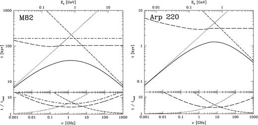
Comparison of the e± loss times from different processes in an M 82-like starburst (left) and in an Arp 220-like starburst (right). The total loss time tcool is the solid line, while bremsstrahlung is long-dashed, ionization is dotted, wind losses are long/short-dashed, and synchrotron and IC together are dash-dotted. On the top are the absolute loss times, while on the bottom is the ratio of each individual loss time to the total loss time.
We also consider the radio nuclei of Arp 220, using a magnetic field |${\sim } 2\ \textrm {mG}$| (e.g. Lacki et al. 2010), a density of |${\sim } 10^4\ \textrm {cm}^{-3}$| (Downes & Solomon 1998) and a radiation energy density equivalent to that of a 50 K blackbody (|${\sim } 30000\ \textrm {eV}\ \textrm {cm}^{-3}$|). The loss times for these conditions are shown in the right-hand panel of Fig. 1. At 1 GHz, ionization now is the most important loss: this is because we see lower energy e± with the higher magnetic field strength. Near 10 GHz, though, bremsstrahlung again is the strongest loss, with X ∼ 3.
For other starbursts, we generally expect advection, bremsstrahlung or ionization losses to dominate: advection in low-density starbursts (cf., Crocker et al. 2011), ionization in starbursts with high magnetic fields (likely in the densest starbursts like Arp 220) where we see low-energy e± and bremsstrahlung in intermediate density starbursts. At frequencies where bremsstrahlung dominates, X ≈ 3 (compare with fig. 4, left-hand panel of Lacki et al. 2010). In starbursts where advection is very strong, however, protons are likely to escape rather than produce pionic secondary e±. Since advection is equally strong for protons and e±, the proton to electron ratio is just K0 when primaries dominate the e± spectrum, and the revised equipartition formulae of Beck & Krause (2005) apply.
2.5 The equipartition and minimum-energy formulae
Another possible worry of assuming that UCR = Up is that the CRs include heavier nuclei, especially helium. In the Milky Way, though, the hydrogen/helium ratio at equal rigidities is ∼8, and at equal energies per nucleon, the hydrogen/helium ratio is ∼24 (Webber & Lezniak 1974; Webber, Golden & Stephens 1987). This ratio must be multiplied by the atomic mass A of helium when calculating the energy density, but still helium is only (1/24 − 1/8) × 4 ≈ 1/6 − 1/2 of the CR energy density. Analysis of the CR flux at Earth indicates that helium makes up about ∼1/6 of the Galactic CR energy density, with another ∼1/12 from heavier nuclei (Webber 1998). Furthermore, helium produces pionic secondary e± just as hydrogen does: as far as collisions go, a helium nucleus at high energies is much like a collection of protons with the same energy per nucleon. Nucleons can shield each other in heavy nuclei, reducing the proton–proton (pp) cross-section per nucleon as A−1/4 for an atomic mass A (Orth & Buffington 1976; Strong & Moskalenko 1998), but for helium this just reduces the cross-section by 30 per cent. Therefore, the hadronic starburst radio emission traces high-energy CR helium nuclei as well as CR protons, and our derived Up basically includes the contribution from helium as well.
2.5.1 Bremsstrahlung-scaled losses
The ratio Beq/Bmin is [4/(p + 1)]2/(p + 5), the same as in the revised equipartition formula of Beck & Krause (2005) (see Table 2). When bremsstrahlung losses dominate, the proton to electron ratio is constant with energy, so the proton/electron ratio has the same behaviour as if there are no losses.
2.5.2 Ionization-dominant losses
At low energies, ionization (or Coulomb losses) will always dominate the energy losses of CR e±. For M 82, ionization losses should become most important for e± radiating below |${\sim } 300\ \textrm {MHz}$|, while for Arp 220, ionization losses are most important all the way up to |${\sim } 3\ \textrm {GHz}$| (Fig. 1). This assumption is therefore most appropriate for observations with low-frequency telescopes like LOw Frequency ARray (LOFAR) when they observe starbursts. While more complicated to scale from pionic losses, because the ionization losses depend on electron energy, at sufficiently low energies they will be the only loss, making the calculation of the electron spectrum relatively simple.
2.5.3 Synchrotron-dominant losses
At high energies, synchrotron and IC losses always dominate the cooling of CR e±. For M 82, this should happen for e± emitting above |${\sim } 5\ \textrm {GHz}$| and for Arp 220, the transition is for e± emitting above |${\sim } 15\ \textrm {GHz}$| (Fig. 1). In order for the observed infrared-radio correlation to hold for starbursts, it is thought that UB ≈ Urad in starbursts (Völk 1989; Condon et al. 1991; Lacki et al. 2010). Therefore for high-frequency radio emission, it may be more convenient to scale to the synchrotron lifetime. This case was previously considered in Pfrommer & Enßlin (2004), but we rederive it with our more approximate approach to compare with the other formulae. Synchrotron losses do not depend on density, so the density dependence in tπ is not cancelled out.
The resulting energy densities and magnetic fields are much smaller than the bremsstrahlung estimates. This is because the synchrotron cooling alone is relatively slow compared to pionic cooling for the parameters used. Thus, the pionic e± accumulate longer, leading to a smaller proton/electron ratio. With less ‘invisible’ CR proton content compared to CR e± content, the energy density is smaller.
Ratio of equipartition and minimum-energy magnetic fields.
| Formula | |$\displaystyle \frac{B_{\rm eq}}{B_{\rm min}}$| | |$\displaystyle \frac{B_{\rm eq}}{B_{\rm min}} (p = 2.0)$| | |$\displaystyle \frac{B_{\rm eq}}{B_{\rm min}} (p = 2.2)$| | |$\displaystyle \frac{B_{\rm eq}}{B_{\rm min}} (p = 2.4)$| | Reference |
|---|---|---|---|---|---|
| Classical formula | [4/3]2/7 | 1.09 | – | – | Beck & Krause (2005) |
| Revised formula | [4/(p + 1)]2/(p + 5) | 1.09 | 1.06 | 1.04 | Beck & Krause (2005) |
| Hadronic formulae | |||||
| Bremsstrahlung-scaled losses | [4/(p + 1)]2/(p + 5) | 1.09 | 1.06 | 1.04 | Section 2.5.1 (equations 33 and 36) |
| Ionization-dominant losses | [4/p]2/(p + 4) | 1.26 | 1.22 | 1.17 | Section 2.5.2 (equations 42 and 45) |
| Synchrotron-dominant losses | [4/(p − 2)]2/(p + 2) | ∞a | 4.2 | 2.8 | Section 2.5.3 (equations 49 and 52) |
| IC-dominant losses | [4/(p + 2)]2/(p + 6) | 1.0 | 0.99 | 0.98 | Section 2.5.4 (equations 58 and 61) |
a As discussed in Section 2.5.3, in practice this limit can never be attained, because of breaks in the CR spectrum, non-steady-state effects and other radiative losses that become important when B is low.
2.5.4 IC-dominant losses
3 APPLYING THE EQUIPARTITION FORMULA
3.1 How much of the radio flux is diffuse and non-thermal?
So far, we have been assuming throughout the paper that all of a starburst's GHz radio flux is diffuse synchrotron emission from CR e± in the interstellar medium. We also assumed that the synchrotron flux is transmitted freely to Earth. Neither is completely true, although it turns out these are often reasonable approximations.
At high frequencies, thermal free–free emission, which does not trace magnetic fields or CRs, becomes increasingly important, since it has a flat ν−0.1 spectrum. However, the total amount of free–free emission is limited by the number of ionizing photons generated by the starburst. At 1.4 GHz, the thermal fraction is at most ∼1/8 for starbursts that lie on the observed infrared-radio correlation, as estimated by Condon (1992); if many ionizing photons escape the starburst or are destroyed by dust do not contribute, the thermal fraction might be smaller. A few very young starbursts appear to have no synchrotron flux, perhaps because supernovae have not gone off in them (Roussel et al. 2003), but most star-forming galaxies and starbursts have radio spectral indices ≪−0.1, indicating non-thermal emission dominates the GHz flux (e.g. Klein, Wielebinski & Morsi 1988; Condon 1992; Niklas, Klein & Wielebinski 1997; Clemens et al. 2008; Ibar et al. 2010; Williams & Bower 2010). Radio spectrum fits to normal spiral galaxies indicate that their typical 1.4 GHz thermal fraction is ∼10 per cent (Niklas et al. 1997). For starburst galaxies, the spectral fits are more difficult, because the transition between the different cooling processes at different frequencies cause the intrinsic synchrotron spectrum to steepen (Thompson et al. 2006), whereas free–free emission flattens the spectrum; disentangling the effects of the two is difficult (Condon 1992). Model fits to starburst radio spectra so far generally indicate GHz thermal fractions of a few per cent (e.g. Klein et al. 1988; Williams & Bower 2010). We adopt |$f_{\rm therm} = [9 (\nu / \textrm {GHz})^{-0.6} + 1]^{-1}$|, which is appropriate if the non-thermal synchrotron spectrum has a ν−0.7 spectrum and the thermal fraction at 1 GHz is 10 per cent.
The same ionized matter that generates free–free emission must also have free–free absorption on some level, but the effects of absorption are harder to calculate because it depends on the geometry of the ionized gas. The simplest approach to estimate the free–free absorption from the radio spectrum is with uniform slab models, in which the synchrotron-emitting CRs and ionized 104 K gas are assumed to be homogeneous and fully mixed. With uniform slab models, the free–free turnovers are generally expected to be in the range of a few hundred MHz for M 82 and NGC 253's starburst cores, with optical depths of the order of ∼0.1 at 1 GHz (Carilli 1996; Williams & Bower 2010; Adebahr et al. 2012). Free–free absorption may be important for frequencies up to a few GHz in Ultraluminous Infrared Galaxies (ULIRGs; Condon et al. 1991; Torres 2004; Clemens et al. 2008). In either case, free–free absorption might significantly suppress the observed synchrotron luminosity at frequencies where ionization cooling dominates.
Yet, the ionized gas is not likely to be uniformly distributed in the starburst. Much of the ionized mass instead is likely concentrated discrete H ii regions, which are dense but have small filling factor. Since not all sightlines through the starburst necessarily pass through an H ii region, it is possible that some synchrotron flux is transmitted even as the frequency descends deep into the MHz range (Lacki 2012). Radio recombination line observations are often interpreted with models of H ii regions. These studies find H ii regions of a wide range of densities in starbursts, but generally fall into the categories of relatively low-density (|${\sim } 1000\ \textrm {cm}^{-3}$|) regions with relatively high-covering fractions and relatively high-density (|${\sim } 10^5\ \textrm {cm}^{-3}$|) regions with relatively low-covering fractions (Anantharamaiah et al. 1993; Rodriguez-Rico et al. 2004; Rodríguez-Rico et al. 2006). In Arp 220, the high-density H ii regions are opaque even past 10 GHz, but they cover only a fraction of a per cent of the starburst; a more diffuse component of ionized gas has an optical depth of ∼10 per cent at 8 GHz (Anantharamaiah et al. 2000).
Given the difficulty of accurate calculations of free–free absorption, the relatively weak dependence of the equipartition and minimum-energy estimates on the flux, the uncertainty in other factors like emitting volume (both because of projection effects and because of the unknown value of the CR filling factor) and the fact that free–free absorption optical depth is expected to be significantly less than one at the frequencies we consider (1–1.4 GHz for most starbursts, 8.4 GHz for ULIRGs); we ignore it when estimating the magnetic fields and CR energy densities below. However, its effects should be considered carefully when working at low frequencies with the ionization-dominant losses formulae.
Finally, not all of the synchrotron flux comes from the CRs in the starburst interstellar medium. First, some of the radio emission actually comes from individual radio sources like supernovae remnants. The fraction of the flux from these individual sources is only a few per cent of the total starburst flux, though, so we ignore it (Lisenfeld & Völk 2000; Lonsdale et al. 2006). Secondly, not all of the flux comes from the starbursting region itself, where the CRs are accelerated or created through pion production, and where the magnetic and CR energy densities are thought to be the highest. Some comes from the surrounding host galaxy and additional emission can arise from a ‘halo’ region thought to arise when CR e± are advected away from the galaxy. In the case of NGC 253, about half of the radio flux in fact comes from these regions rather than the starburst core, so we use the core flux only (Heesen et al. 2009; Williams & Bower 2010). Likewise, in NGC 1068, most of the radio flux comes from an active nucleus and its jets, so we use the estimated flux of the starburst alone (Wynn-Williams, Becklin & Scoville 1985). We assume in the other cases that all of the synchrotron flux comes from the starburst core, but this can be tested with resolved observations. This is known to be a reasonable approximation for M 82, where the starburst core does actually dominate the total flux at frequencies above 1 GHz (Adebahr et al. 2012).
3.2 New equipartition estimates of B in starbursts
We present new equipartition estimates of the magnetic field strength in selected starburst galaxies in Table 3. These estimates use the bremsstrahlung-dominated formula with X = 3, and also assume that p = 2.2 and f|${^{CR}_{fill}}$| = fsec = ζ = 1. For comparison, we also give the results for the classical and revised equipartition formula. Note that we use 8.4 GHz radio data for the ULIRGs Arp 220, Arp 193 and Mrk 273; at these higher frequencies, bremsstrahlung still should be the most important loss (Fig. 1, right-hand panel).
Updated equipartition estimates for starbursts.
| Starburst | D | R | h | ν | Sν | Bremsstrahlung-scaleda | Classicalb | Revisedc | Referencesd | |||
|---|---|---|---|---|---|---|---|---|---|---|---|---|
| UCR | Beq | Bmin | Bmin | Beq | Bmin | |||||||
| (Mpc) | (pc) | (pc) | (GHz) | (Jy) | (eV cm−3) | (|$\mu \textrm {G}$|) | (|$\mu \textrm {G}$|) | (|$\mu \textrm {G}$|) | (|$\mu \textrm {G}$|) | (|$\mu \textrm {G}$|) | ||
| M 82 | 3.6 | 250 | 50 | 1.0 | 8.94 | 940 | 190 | 180 | 160 | 240 | 220 | (1) |
| NGC 253 Core | 3.5 | 150 | 50 | 1.0 | 3.0 | 880 | 190 | 180 | 160 | 230 | 220 | (1) |
| NGC 4945 | 3.7 | 540 | 50 | 1.4 | 4.2 | 300 | 110 | 100 | 89 | 130 | 130 | (2) |
| NGC 1068 Starburst | 13.7 | 3000 | 50 | 1.4 | 1 | 86 | 59 | 55 | 47 | 72 | 68 | (3) |
| IC 342 | 4.4 | 710 | 50 | 1.4 | 2.25 | 190 | 87 | 82 | 71 | 110 | 100 | (4) |
| NGC 2146 | 12.6 | 520 | 50 | 1.4 | 1.09 | 570 | 150 | 140 | 130 | 190 | 180 | (4) |
| NGC 3690 | 42.2 | 2460 | 50 | 1.4 | 0.66 | 300 | 110 | 100 | 89 | 130 | 130 | (4) |
| NGC 1808 | 14.2 | 1030 | 50 | 1.4 | 0.52 | 200 | 91 | 85 | 73 | 110 | 100 | (4) |
| NGC 3079 | 15.9 | 190 | 50 | 1.4 | 0.85 | 2000 | 280 | 270 | 240 | 350 | 330 | (4) |
| Arp 220 West | 75 | 100 | 50 | 8.4 | 0.072 | 9300 | 610 | 580 | 500 | 750 | 710 | (5) |
| Arp 220 East | 75 | 100 | 50 | 8.4 | 0.061 | 8500 | 590 | 550 | 480 | 720 | 670 | (5) |
| Arp 193 | 99 | 160 | 50 | 8.4 | 0.035 | 5000 | 450 | 420 | 360 | 550 | 520 | (4) |
| Mrk 273 | 160 | 160 | 50 | 8.4 | 0.044 | 9800 | 630 | 590 | 510 | 770 | 720 | (4) |
Columns: D is the distance to the starburst; R is the assumed radius of the starburst disc and h is the assumed midplane-to-edge scale height of the starburst disc, for a total volume of V = 2πR2 h; Sν is the total observed flux density at frequency ν. We take the thermal fraction of the radio emission to be |$f_{\rm therm} = [9 (\nu / \textrm {GHz})^{-0.6} + 1]^{-1}$|.
a Equipartition energy densities, equipartition magnetic field strengths and minimum-energy magnetic field strengths calculated assuming radio emission is hadronic and with e± lifetimes scaled to the bremsstrahlung loss time, from equations (32), (35) and (36). We assume X = 3, fsec = 1, f|${^{CR}_{fill}}$| = 1, ζ = 1 and p = 2.2.
b Classical minimum-energy estimate of magnetic field strength from Longair (2010), which assumes K0 = 100, νmin = ν and α = 0.75.
c Revised equipartition and minimum-energy magnetic field strengths from Beck & Krause (2005), which assumes p = 2.2 (synchrotron spectral index α = 0.6) and K0 = 100.
d References – (1) M 82 and NGC 253 radio flux densities from Williams & Bower (2010); (2) NGC 4945 radio flux density and size from Strickland et al. (2004); (3) radio flux density and approximate radius of NGC 1068 starburst from Wynn-Williams et al. (1985); (4) radio flux densities and radii compiled from Thompson et al. (2006); (5) distance and sizes of Arp 220's radio nuclei from Sakamoto et al. (2008); radio flux density from Thompson et al. (2006).
The equipartition magnetic field strengths range from 60 to 600 |$\mu \textrm {G}$|. For M 82 and NGC 253, the estimated magnetic fields are |$200\ \mu \textrm {G}$|, which is entirely in line with broad-band modelling of their non-thermal spectra (e.g. de Cea del Pozo et al. 2009a). Klein et al. (1988) and Adebahr et al. (2012) found smaller magnetic field strengths of 50–100|$\ \mu \textrm {G}$|, but they assumed that the emission was spread over a larger volume so that the energy densities were smaller. The magnetic field strength estimates for the distant ULIRGs such as Arp 220 are of the order of half a milliGauss, which is several times smaller than the few milliGauss expected from the linearity of the FIR-radio correlation (Condon et al. 1991; Lacki et al. 2010) and detailed modelling of Arp 220's CR population (Torres 2004). The derived magnetic field strengths depend weakly on ζ = UB/UCR, though, with B ∝ ζ2/(5 + p) and UCR ∝ ζ−(1 + p)/(5 + p) for the bremsstrahlung-loss formulae. At a given radio flux, and if no other assumptions are changed, magnetic field strengths that are three times stronger than equipartition require ζ ≈ 50 and CR energy densities six times smaller than the values derived for ζ = 1.
However, the most interesting feature of the new equipartition estimates evident in Table 3 is that they are still of the same order as the classical and revised equipartition and minimum-energy estimates.
3.3 Why do previous equipartition formulae seem to work?
If previous equipartition formulae do not apply to starbursts, because of starbursts’ strong electron cooling and the presence of secondary e±, why do these formulae give similar results to the corrected formula?
The reasons the assumption works are as follows:
While synchrotron and IC strongly suppress the proton/electron ratio at high energy and while ionization losses strongly suppress the proton/electron ratio at low energy, bremsstrahlung-dominated losses roughly preserve the proton/electron ratio, since tπ/tbrems ≈ 1.6. Although bremsstrahlung is more important at high density, reducing the steady-state electron density (Beck & Krause 2005); the pionic losses also scale with density, reducing the steady-state proton density.
At 1 GHz, we are observing at intermediate energies in starbursts, a sweet spot where none of the other losses greatly overpowers bremsstrahlung. But while bremsstrahlung may be the strongest individual loss, the other losses combined are more important than bremsstrahlung (X ≈ 3). As seen in Fig. 1, the e± radiative lifetime reaches a maximum for energies observed at GHz frequencies. So the combined effect of the losses is to suppress the proton/electron ratio, but only by a factor of ∼5.
On the other hand, the proton/electron injection ratio is raised by a factor of ∼5 due to the presence of pionic secondaries. The ‘dilution’ effect arising because secondary e± are injected at much lower energy than the primary protons helps ensure that the secondaries do not swamp the electron population.
This is related to the ‘high-Σg conspiracy’ posited by Lacki et al. (2010) to explain the FIR-radio correlation from normal galaxies to starbursts: radio emission is enhanced by secondaries, but is suppressed by non-synchrotron losses including bremsstrahlung.
A consequence is that if we move to higher or lower electron energy (or observing frequency), X will increase beyond ∼3. The coincidence no longer works and the proton/electron ratio is increased by either ionization losses at low frequency or synchrotron and IC losses at high frequency. At sufficiently low energies (|$\lesssim 100\ \textrm {MeV}$|; observed |$\lesssim 40\ \textrm {MHz}$| in the M 82 and NGC 253 starbursts), the pionic secondary spectrum will also subside due to the kinetics of pion production. At low frequencies, such as those observed by LOFAR, both of these effects can increase the proton/electron ratio above that of the hadronic bremsstrahlung-losses case. At a few hundred MHz, where the secondaries are present, the ionization-loss formulae (Section 2.5.2) should work since it already takes into account the changing proton/electron ratio. The assumption of a CR proton injection spectrum of the form of a E− p power law also probably starts to break down at proton energies of a GeV as well, with a momentum power law or some non-linear acceleration spectrum likely more appropriate.
However, while these effects formally invalidate the bremsstrahlung-loss dominated formula outside of the frequency range where bremsstrahlung losses dominate (300 MHz to 6 GHz for M 82; 3 GHz to 15 GHz in Arp 220's nuclei), in practice, their effects are relatively benign. From the classical and revised formulae, the proton/electron ratio affects the magnetic field strength estimates only approximately as K|${^{2/7.2}_{0}}$|: an order of magnitude change in K0 only results in a factor of ∼2 change in Bmin or Beq. At low frequencies, the ratio of ionization to bremsstrahlung loss times only goes as tion/tbrems ∝ ν1/2, and the proton/electron ratio varies similarly. To take an extreme example, M 82's radio flux at 22.5 MHz is 39 Jy (Roger, Costain & Stewart 1986). Naively putting these values into the bremsstrahlung loss formula (and assuming all of this flux comes from the starburst region) gives |$B_{\rm eq} = 170\ \mu \textrm {G}$| and |$B_{\rm min} = 160\ \mu \textrm {G}$| – values that are within ∼25 per cent of those obtained using the formula at 1 GHz. The more formally correct ionization-loss formulae instead give |$B_{\rm eq} = 180\ \mu \textrm {G}$| and |$B_{\rm min} = 140\ \mu \textrm {G}$|.
4 CONCLUSION
We rederive minimum-energy and equipartition estimates for the magnetic fields for the conditions that prevail in starburst galaxies. In these galaxies, the radio-emitting CR e± population may consist largely of hadronic pp secondaries rather than primaries. Furthermore, strong radiative losses, particularly bremsstrahlung at GeV energies, set the lifetime of the CR e± and affect the proton/electron ratio. Despite these effects, we found that the steady-state proton/electron ratio is probably close to ∼100 for GHz-emitting e±, assuming that tbrems ≈ 3te. As a result, the classical and revised equipartition formulae give results that are quite similar to ours, despite their different assumptions.
Although we scale the CR e± lifetime to individual losses (particularly bremsstrahlung) to derive an analytical result, it should also be possible to numerically solve for Beq and Bmin using the full expression for tcool including all losses, if equation (19) is used. However, since the density would not fully cancel out (due to synchrotron and IC losses in the e± lifetime) and because the IC lifetime depends on the radiation energy density, such an estimate would require both the gas density the CRs experience and the radiation energy density.
While our focus has been on starburst galaxies, the formulae above should apply for any radio source where the CR e± population is mostly pionic pp secondaries and is strongly cooled. Pfrommer & Enßlin (2004) already considered the case of radio emission from galaxy clusters, which may come from secondary e± (Dennison 1980) that cool from synchrotron and IC losses off the CMB over the Gyr lifetimes of clusters. Active galactic nuclei may also accelerate CR protons when their jets are stalled by surrounding gas (e.g. Alvarez-Muñiz & Mészáros 2004). These protons may interact with the gas to produce pionic secondaries, which may radiate in the radio; the formulae derived here would also apply in such a case.
BCL was supported by a Jansky fellowship from the National Radio Astronomy Observatory (NRAO). NRAO is operated by Associated Universities, Inc., under cooperative agreement with the National Science Foundation. RB acknowledges financial support from grant DFG FOR1254. BCL acknowledges earlier discussions with Todd Thompson. We also thank Marita Krause for comments on the manuscript.
Jansky Fellow of the National Radio Astronomy Observatory.
When neither CR protons nor CR e± are cooled, the minimum-energy and equipartition magnetic field strengths are equal if CRs are injected with a spectral index of 3 (Beck & Krause 2005).
We assume that both the gas and the synchrotron-emitting CRs have the same scale height h, since secondary e± are created by interactions of CR protons with gas and the CR e± lifetimes are short in starbursts.
