A theory of photospheric emission from relativistic, collimated outflows

Abstract

1 INTRODUCTION

Photospheric emission from highly relativistic outflows was early considered as an explanation for prompt gamma-ray bursts (GRBs; Goodman 1986; Paczyński 1986). It is a natural consequence of the fireball model, where the optical depth at the base of the outflow is much larger than unity (e.g. Piran 1999). Moreover, photospheric emission provides a natural explanation to the small dispersion of the sub-MeV peak and to the high prompt emission efficiency observed (Mészáros & Rees 2000). However, the observed spectrum usually appears significantly broader than a Planck spectrum (Preece et al. 2000), being well fitted by a smoothly broken power law (the Band function, Band et al. 1993). Thus, the prompt emission has commonly been associated with synchrotron emission originating from kinetic energy dissipation outside the photosphere (Rees & Mészáros 1994). However, in recent years it has become clear that optically thin synchrotron emission is incompatible with the hard low-energy slopes observed in a substantial fraction of GRBs (Preece et al. 1998; Kaneko et al. 2006; Beloborodov 2012). This has raised the need for alternative ideas.

One appealing idea is broadening of the thermal spectrum emitted from the photosphere. The emerging photon spectrum from a static, optically thick, relativistic outflow can be widened in two ways.

• Energy dissipation below the photosphere can heat electrons above the equilibrium temperature. These electrons emit synchrotron emission and Comptonize the thermal photons, thereby modifying the Planck spectrum (Pe'er, Mészáros & Rees 2005, 2006; Rees & Mészáros 2005). The dissipation can be caused by shocks (Rees & Mészáros 2005; Lazzati, Morsony & Begelman 2009; Ryde et al. 2011), dissipation of magnetic energy (Thompson 1994; Spruit, Daigne & Drenkhahn 2001; Giannios & Spruit 2005; Zhang & Yan 2011) or collisional processes (Beloborodov 2010; Vurm, Beloborodov & Poutanen 2011).

• The photospheric radius is angle-dependent (Abramowicz, Novikov & Paczynski 1991; Pe'er 2008). Moreover, it was shown by Pe'er (2008) that photons make their last scatterings at a distribution of radii and angles. The observer sees simultaneously photons emitted from a large range of radii and angles. Therefore, the observed spectrum is a superposition of comoving spectra. The Doppler boost is a function of angle, and the comoving temperature decreases with radius through adiabatic cooling. Depending on the outflow properties, this geometrical broadening can form observed spectra which appear significantly different from the Planck spectrum.

Photospheric emission in the context of spherically symmetric outflows has been studied by several authors. Goodman (1986) considered a highly relativistic outflow in the context of cosmological GRBs. It was realized that the observed spectrum is broader than blackbody; however, the analysis was one dimensional. Abramowicz et al. (1991) realized that the 2D shape of the photosphere in a relativistic, spherically symmetric wind is in fact concave and symmetric around the line of sight (LOS). This can be understood as a consequence of the dependence on viewing angle of the optical depth of relativistically moving media. Pe'er (2008) found a simple expression for the photospheric radius, R_ph ∝ (θ²/3 + 1/Γ²), where θ is the angle measured from the LOS, Γ ≡ (1 − β)^−1/2 is the outflow bulk Lorentz factor and β is the outflow speed in units of the speed of light. Pe'er (2008) extended the photospheric emission model by recognizing the importance of considering photons from the entire emitting volume, introducing probability density distributions for the last scattering photon positions. Beloborodov (2011) took a different approach, solving the radiative transfer equation in the relativistic limit. The approximate probability densities used by Pe'er (2008) were validated by Beloborodov (2011).

All above-mentioned works considered spherical explosions. As we show below, this is a good approximation for collimated outflows as long as the characteristic jet opening angle is much larger than 1/Γ, and the outflow is observed at viewing angles much smaller than the jet opening angle. Within the collapsar model (MacFadyen & Woosley 1999), the jet is collimated by the pressure of the surrounding gas as it drills its way through the collapsing progenitor star. In such jets the position of the observer relative to the jet axis can affect the observed spectrum. Here we develop the theory of photospheric emission in collimated outflows, calculating the expression for the observed spectrum at any viewing angle.

The mechanism responsible for jet collimation is not fully understood. Hydrodynamic simulations of GRB jets after the launching phase (e.g. Zhang, Woosley & MacFadyen 2003; Morsony, Lazzati & Begelman 2007; Mizuta, Nagataki & Aoi 2011) show the jet drilling through the stellar envelope, pushing material towards the sides, forming a hot cocoon (e.g. Aloy et al. 2000). The surrounding gas then acts to collimate the jet. Zhang et al. (2003) extracted angular profiles of the local rest-mass density, total energy flux and outflow Lorentz factor at certain radii from the simulations. The resulting profiles can in many cases be approximated as constant within a characteristic jet opening angle, then decreasing as power laws towards the jet edge. In this work we adopt a similar parametrization of the angular profile of the bulk jet Lorentz factor, with a characteristic jet opening angle, power-law index and normalization as free profile parameters.

We develop a model for photon propagation in the context of a steady, optically thick, axisymmetric jet with angle-dependent electron number density, photon number density and bulk Lorentz factor. We compute the observed spectrum taking into account contributions from the entire emitting volume as seen by an observer located at any viewing angle. As an example solution, we consider fireball dynamics as a way to relate the angle-dependent parameters, in combination with the assumed angular Lorentz factor profile. We developed a Monte Carlo simulation, unique in its ability to calculate photon propagation in a non-spherical explosion. We use this simulation to analyse the importance of angular bulk photon diffusion.

We show that for a large region in the parameter space, the low-energy photon index is approximately α ≈ −1 (where dN/dE ∝ E^α). This is similar to the average value observed in GRBs (Kaneko et al. 2006; Nava et al. 2011; Goldstein et al. 2012). Furthermore, we present analytical expressions for the important energies and photon indices of the observed spectrum as functions of the free model parameters. We show that photospheric emission by itself can account for observations of GRB spectra below the peak energy without the need for energy dissipation below the photosphere or additional radiative processes, provided that the characteristic jet opening angle is not much larger than ∼few/Γ or if the outflow is viewed off-axis. Although we focus on GRB parameters, the results are general and can readily be applied to any optically thick, relativistic outflow with lateral outflow properties such as active galactic nuclei.

This paper is organized as follows. In Section 2 we develop the analytical expression for the observed spectrum. We qualitatively explain the spectral features in Section 3 in terms of contributions from different jet regions. The Monte Carlo code is explained in Section 4, and in Section 5 we present both simulated and numerically integrated spectra for outflow parameters relevant to GRBs. We discuss model sensitivity and photon time delays in Section 6 and summarize our results in Section 7.

2 MODEL: PHOTON SCATTERING IN A STEADY JET

where Γ₀ is the maximum value of the Lorentz factor, θ_j is the characteristic jet opening angle, p determines the gradient of the profile and Γ_min = 1.2 is the lowest value of the Lorentz factor, differing from unity for numerical reasons.¹

Three angular regions can be identified: the inner jet, the outer jet and the envelope. While this separation is artificial and a consequence of our chosen Lorentz factor profile, it is useful for understanding the resulting observed spectra. The inner jet is characterized by an approximately constant Lorentz factor, Γ = Γ₀. In the outer jet the Lorentz factor decreases approximately as a power law of the angle with index p, and in the envelope the Lorentz factor has an approximately constant value of Γ ≈ 1. A characteristic angle separating the inner and outer jet regions is θ_j, where |$\Gamma (\theta _{\rm j}) \approx \Gamma _{\rm 0}/\sqrt{2}$|⁠. Similarly, θ_e ≈ θ_jΓ^1/p₀ is a characteristic angle separating the outer jet and the envelope regions.² An example Lorentz factor profile is shown in Fig. 1.

Figure 1.

Open in new tabDownload slide

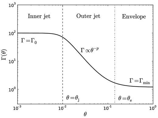
An example Lorentz factor profile (equation 1). In the inner jet (θ < θ_j) the Lorentz factor is approximately constant, Γ = Γ₀, while in the outer jet (θ_j < θ < θ_e) the Lorentz factor decrease is approximately that of a power law with index −p. In the envelope (θ > θ_e), the Lorentz factor is approximately constant with a value of Γ_min = 1.2. The dashed vertical line indicates θ_j, while the dot–dashed line shows the location of θ_e ≈ θ_jΓ^1/p₀. For this figure, Γ₀ = 100, θ_j = 0.01 and p = 2.

Figure 2.

Open in new tabDownload slide

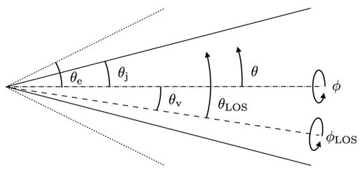
Schematic view of the jet. The solid lines represent the characteristic jet opening angle, θ_j, as measured from the jet axis of symmetry, indicated by the dot–dashed line. The dotted line shows θ_e, the characteristic angle separating the outer jet and the envelope. The dashed line is the LOS, at an angle θ_v to the jet axis. Note that in general, θ_LOS ≠ θ + θ_v.

Physical properties of the jet are expressed in spherical coordinates (r, θ, ϕ), with the polar axis aligned to the jet axis of symmetry (see Fig. 2). Some properties, such as the Doppler boost, depend on the angle to the LOS. These are most easily expressed in spherical coordinates (r, θ_LOS, ϕ_LOS), with the polar axis aligned to the LOS. The radial coordinate (r) is measured along an axis that makes an angle θ with the jet axis and θ_LOS with the LOS. When viewing the jet head-on, the two sets of coordinates coincide, and the radiative contributions from the jet are independent of azimuthal angle due to symmetry around the LOS. Our jet profile contains four parameters (including the viewing angle), three more than the simplified scenario of spherical symmetry.

2.1 The photosphere and the decoupling radius

The photospheric radius, R_ph, is defined as the radius which fulfils the following condition: the optical depth for a photon that propagates from that radius towards the observer is equal to unity. Thus, the photospheric radius defines a surface in space. The radial coordinate of this surface is R_ph = R_ph(θ_LOS, ϕ_LOS). From any point on this surface, the optical depth as measured towards the observer equals unity. In order for a photon to reach the observer, it has to propagate along a ray parallel to the LOS. Along such a ray, |$r \sin \theta _{\rm LOS} = \text{const}$|⁠. We define the z-axis along this ray; z ≡ rcos θ_LOS is the spatial photon coordinate. For the parameter values considered in this work, the comoving temperature at all relevant radii is much lower than the electron rest-mass energy, and so we use the Thomson cross-section in describing the scattering process. The optical depth from z = z_min to z → ∞ is |$\tau _{\rm ray} \equiv \int _{z_{\rm min}}^\infty n_{\rm e}^\prime \sigma _{\rm T} \mathcal {D}^{-1} \text{d}z$|⁠, where |$\mathcal {D} = [\Gamma (1-\beta \cos \theta _{\rm LOS})]^{-1}$| is the Doppler boost, n′_e is the comoving electron number density and σ_T is the Thomson cross-section (Abramowicz et al. 1991; Pe'er 2008). The photospheric radius is a function of angle to the LOS, as follows from the definition of τ_ray. For a spherically symmetric outflow, due to symmetry, the shape of the photosphere is independent of viewing angle. In this work we consider jetted outflows, for which this is no longer true.

Here, in addition, we define the decoupling radius, R_dcp, as the radius from which the optical depth for a photon that propagates in the radial direction is equal to unity. The optical depth from r = r_min to r → ∞ is τ_rdl ≡ ∫^∞_rminΓ(1 − β)n′_eσ_T dr. The importance of R_dcp is that this is the characteristic radius where photons and electrons fall out of thermal equilibrium. If the outflow has axisymmetric comoving electron density or bulk Lorentz factor, then R_dcp is a function of angle to the axis of symmetry. For photons propagating along the LOS (cos θ_LOS = 1), dz = dr and R_ph = R_dcp.

2.2 Formation of the observed spectrum

In order to calculate the observed spectrum, we consider the following: while the photosphere is defined as R_ph = r(τ_ray = 1), in reality photons can scatter anywhere electrons exist. Since we consider an expanding plasma in a steady state, electrons are assumed to occupy the entire volume.³ In order to calculate the observed spectrum one has to integrate the emissivity over the entire volume, where the emissivity in volume element dV is proportional to the probability of photons to make their last scattering in dV.

We assume that the local, comoving photon energy distribution is well described by a Planck spectrum with temperature equal to the local, comoving electron temperature.⁴ As we consider the photon–electron cross-section to be energy-independent, it follows that the optical depth is also energy-independent. In this section we calculate the observed spectrum assuming that it depends only on the last scattering positions of the observed photons. We justify this assumption by simulations (Section 4) which consider full treatment of photon propagation below the photosphere.

2.3 Angle-dependent jet properties

We choose to define Γ = Γ(θ) as given by equation (1), and so |${\rm d}\dot{M}(\theta )/{\rm d}\Omega$| follows from equation (11). Due to adiabatic energy losses the comoving temperature above saturation decreases as T^′ = T₀(r₀/r_s)(r_s/r)^2/3, where r_s = ηr₀ is the saturation radius.

3 CONTRIBUTIONS FROM DIFFERENT JET REGIONS TO THE OBSERVED SPECTRUM

The observed spectrum is obtained by solving equation (10), namely integrating the emissivity over the entire volume. While analytical integration is difficult for the different jet profiles, numerical integration is straightforward. In Sections 3–3.3 we assume the outflow to be viewed head-on. Therefore, the radiative contributions from the different parts of the jet are symmetric around the LOS, and equation (10) is readily integrated over azimuthal angle. Non-zero viewing angles are discussed in Section 3.4 and further explored numerically in Section 5.

In Fig. 3 we present the numerically integrated spectrum where we have used the Lorentz factor profile defined in equation (1). For this figure we use the parameters Γ₀ = 100, θ_j = 0.03 and p = 4, as well as θ_v = 0. The spectrum has a wavy shape, with a slope of roughly F_E ∝ E⁰ over approximately six orders of magnitude in energy, which does not resemble the Planck spectrum. We identify several characteristic photon energies in the spectrum (⁠|$E_{\rm peak}, \, E_{\rm j}, \, E_\mathcal {D}, \, E_{\rm e}$| and E_env). Analytical expressions for these energies are given below.

Figure 3.

Open in new tabDownload slide

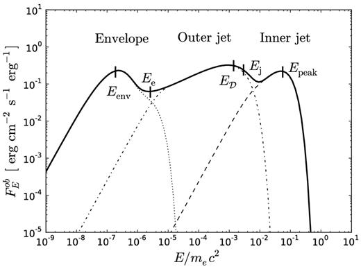
The observed spectrum from a relativistic, optically thick outflow obtained by numerical integration of equation (10). Zero viewing angle is assumed. Separate integration of the contributions from the inner jet, outer jet and envelope is shown with dashed, dot–dashed and dotted lines, respectively. Photon energies associated with characteristic outflow angles are indicated by small vertical lines. For this figure Γ₀ = 100, θ_j = 0.03 and p = 4. A total outflow luminosity of L = 10⁵² erg s⁻¹ and base outflow radius r₀ = 10⁸ are used.

The spectrum can be understood as a combination of components originating from different jet regions. Spectra integrated separately between the angular limits for the inner jet, outer jet and envelope regions are shown in Fig. 3 as dashed, dot–dashed and dotted lines, respectively. The advantage of considering the emission from different jet regions separately is that it allows for analytical expressions of key spectral features.

While the integration is over the entire volume, in order to explain the spectrum one can define characteristic photon energies as a function of angle to the jet axis. This is done in the following way. Consider only photons that make their last scattering between angles θ and θ + dθ. The distribution of last scattering radii spans a large range of radii (see Fig. 4, right-hand panel). At r ≪ R_ph the flux is attenuated by the large optical depth, while at r ≫ R_ph the probability of scattering is low due to the optical depth being much smaller than unity. Therefore, the characteristic radius of the radial distribution is R_ph(θ). The distribution of observed energies of photons that make their last scattering between angles θ and θ + dθ peaks at |$E \approx 2.7 kT^{\rm ob} = 2.7 \, \mathcal {D}(\theta , \Gamma ) \, kT^\prime (\theta , R_{\rm ph}(\theta ))$|⁠. Therefore, one may consider E(θ) = 2.7kT^ob(θ, R_ph(θ)) to be the characteristic energy of photons making their last scattering between angles θ and θ + dθ. Typically, the Doppler boost decreases with angle, while the photospheric radius increases with angle.⁶ Therefore, the characteristic photon energy is expected to decrease with angle. Below we use this approximation to obtain the characteristic photon energies shown in Fig. 3. For θ_v > 0, this discussion has to be generalized to include azimuthal angle.

3.1 Inner jet component

Emission from the inner jet region (0 ≤ θ ≤ θ_j) is shown with a dashed line in Fig. 3. The most energetic part of the spectrum originates from this region due to the high Doppler boost and low photospheric radius (see Fig. 4). Within this region the Lorentz factor is approximately constant. Therefore, the observed spectrum from the inner jet region is similar to that of an optically thick, spherically symmetric wind with Γ ≈ Γ₀ when only considering the emissivity within 0 ≤ θ ≤ θ_j. The Doppler boost, |$\mathcal {D} \approx 2\Gamma /(1 + \Gamma ^2 \theta ^2)$|⁠, and the photospheric radius for a spherically symmetric wind, R_ph ∝ (1 + Γ²θ²/3) (Pe'er 2008), are approximately constant for angles up to θ ≈ 1/Γ₀, and so the characteristic energy of photons making their last scattering within 0 ≤ θ ≤ 1/Γ₀ is approximately constant and is equal to E_peak.

The observed temperature of photons originating from angles larger than 1/Γ₀ decreases with angle due to the increasing photospheric radius and decreasing Doppler boost. For 1/Γ₀ < θ < θ_j, R_ph/R_dcp∝(1 + Γ²₀θ²/3) (see Fig. 4).⁷ Therefore, the approximation of thermal equilibrium close to the photosphere becomes less accurate with increasing angle (within the inner jet region). Since the characteristic photon energy is a monotonically decreasing function of angle for a spherically symmetric outflow, the approximation of thermal equilibrium becomes less accurate with decreasing observed photon energy. By comparing numerically integrated spectra to the full Monte Carlo simulations, we find that for E ≳ 10⁻²E_peak the assumption of thermal equilibrium can be used.

The superposition of comoving spectra causes softening of the Rayleigh–Jeans part of the observed spectrum from the inner jet. Through simulations we find that the spectral index at E = 10⁻²E_peak from a spherically symmetric outflow is approximately 0.6 units softer than the Planck spectrum. This agrees with the index found by Beloborodov (2010) who considered radiative transfer in a spherically symmetric, collisionally heated outflow.

3.2 Outer jet component

The spectrum from the outer jet region (θ_j ≤ θ ≤ θ_e) is shown with a dot–dashed line in Fig. 3. It forms an approximate power law between two limiting energies, E_e and |$E_\mathcal {D}$|⁠. We derive analytical expressions for the power-law index and the upper and lower energy limits below. No simple analytical expression exists for the spectrum within the remaining energy range |$E_\mathcal {D} < E < E_{\rm j}$|⁠. However, this energy range is typically small for the parameter space considered in this work.

Figure 4.

Open in new tabDownload slide

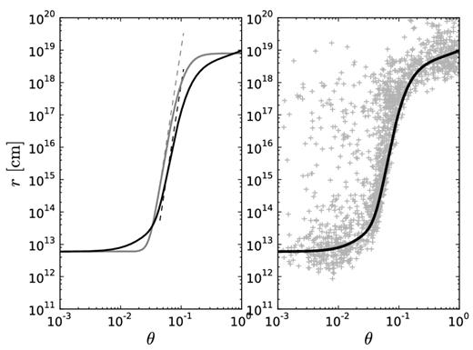
The left-hand panel shows the photospheric radius (R_ph, black) and the photon decoupling radius (R_dcp, grey) as functions of angle. The dashed lines are the power-law approximations used in Section 3.2. The right-hand panel shows the same photospheric radius (black) and Monte Carlo simulations of the photon last scattering positions before reaching the observer (grey) for θ_v = 0 (0.000 ≤ θ_v ≤ 0.006). The Lorentz factor profile Γ₀ = 100, θ_j = 0.03 and p = 4 was used along with θ_v = 0. A total outflow luminosity of L = 10⁵² erg s⁻¹ was assumed in calculating the radii.

Figure 5.

Open in new tabDownload slide

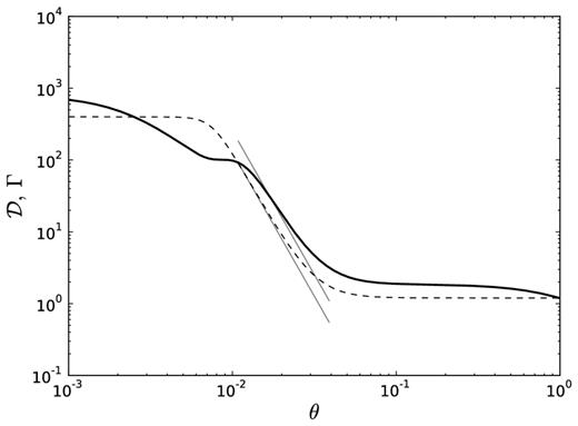
The Doppler boost (solid black) and the Lorentz factor (dashed black) as functions of angle to the jet axis. θ_v = 0 is assumed. The respective approximations used in Section 3.2 are shown as grey lines. The Doppler boost has a bump at angle |$\theta \approx \theta _\mathcal {D}$|⁠. The characteristic photon energy associated with |$\theta _\mathcal {D}$| is shown in Fig. 3. A Lorentz factor profile (equation 1) with parameter values Γ₀ = 400, θ_j = 3/Γ₀ and p = 4 was used.

where x ≡ (3p + 1)^{− 1}(Γ₀θ^p_j)^{− 4}(R_*/r₀)(ϵ/2)^3/2θ^4p, x_min = (3p + 1)^{− 1}(R_*/r₀)(ϵ/2)^3/2(Γ₀θ^p_j)^{4/p − 1} and |$x_{\rm max} = (3p+1)^{-1} (R_{\rm *}/r_{\rm 0})(\epsilon /2)^{3/2} [(1 + \sqrt{2})/\Gamma _{\rm min}]^4$|⁠.

3.3 Envelope component

The spectrum from the envelope component (θ ≤ θ_e) is shown with a dotted line in Fig. 3. It is characterized by a peak at E = E_env, where E_env is given by the observed temperature of the envelope component.

3.4 Non-zero viewing angles

Due to the complexity of the calculation in this scenario, we give here only a qualitative explanation. Full quantitative treatment is presented in Section 5. Increasing the viewing angle has two main consequences: decreasing E_peak (and therefore also the bolometric flux) and softening the spectrum. Since the characteristic angles for the inner jet are smaller than those for the outer jet, the inner jet spectral component is affected more than the outer jet component by viewing angle variations.

As long as θ_v ≪ θ_j, the observed spectrum is well approximated by the θ_v = 0 solution. For θ_v > θ_j, E_peak decreases due to the decreasing Doppler boost as well as the increasing photospheric radius. Photons from the outer jet region contribute to a general softening of the spectrum below the peak energy. For θ_v > θ_j, the total observed flux decreases with increasing viewing angle, and at some viewing angle (dependent on jet parameters as well as detector characteristics) the flux in non-detectable.

For p → ∞, the jet profile approaches a top-hat shape. For such jets the peak energy and bolometric flux decreases rapidly with increasing viewing angle (for θ_v > θ_j), and the probability of observing the outflow at θ_v > θ_j is low. However, for outflows with a shallow Lorentz factor gradient (small values of p), the bolometric flux and peak energy decrease are slower. Therefore, the outflow may be observed up to |$\theta _{\rm v} \approx \text{few} \times \theta _{\rm j}$|⁠, depending on detector characteristics and the exact jet profile. We assume θ_{v, max} to be the largest viewing angle where the outflow is still detectable. The fraction of GRBs observed at θ_v < θ_j is ΔΩ_j/ΔΩ_{v, max} = θ²_j/θ²_{v, max}. For |$\theta _{\rm v, max} > \sqrt{2} \times \theta _{\rm j}$|⁠, the majority of observed outflows are viewed at θ_v > θ_j. Therefore, the consequences of observing the outflow at θ_v ≈ θ_j should not be neglected.

4 NUMERICAL SIMULATION

In order to validate the analytical model and to explore the importance of full photon propagation history, a numerical code has been developed. The code is based on an earlier code for photon propagation in a spherically symmetric, relativistically expanding plasma (Pe'er & Waxman 2004; Pe'er et al. 2006; Pe'er 2008). This code is specially designed to allow for the bulk Lorentz factor, mass outflow rate and photon emission rate to be functions of angle with respect to the jet axis. This is required in the current context as the optical depth between two points in the outflow depends on the local Lorentz factor and electron density. As photons propagate across the jet, photon energy changes due to propagation between regions of different bulk Lorentz factor are inherently considered; therefore, the comoving photon spectrum at the last scattering position is not artificially fixed to blackbody. No assumption of thermal equilibrium is made above the photon injection position, as opposed to the analytical model. The full Klein–Nishina cross-section is used in the scattering process.

4.1 Code description

The code tracks photon propagation, starting from a random position in the outflow with τ_rdl = 20, ensuring a low probability [exp (−20) ≈ 2.1 × 10⁻⁹] for a photon to escape the outflow without being scattered. The lab frame angular coordinates of the initial position are randomly drawn from a uniform distribution. The initial photon propagation direction is randomly chosen in a similar way. The initial comoving photon energy is drawn from a blackbody distribution with temperature equal to the comoving outflow temperature at the photon position: T^′(θ, r) = T₀(r₀/r_s(θ))(r_s(θ)/r)^2/3.

A photon has a probability exp (−τ) to propagate an optical depth τ before scattering. Thus, an optical depth, Δτ, representing the distance between scatterings in the direction of propagation, is drawn from a logarithmic distribution. The optical depth from the photon position to infinity in the photon propagation direction, τ_∞, is calculated and compared to the drawn optical depth. If Δτ ≥ τ_∞, the photon escapes the outflow, else the distance corresponding to Δτ is calculated, taking into account the angular dependence of the Lorentz factor and electron number density. The new photon scattering position is then considered. The photon four-vector is transformed into the local comoving outflow frame. The scattering electron Lorentz factor is drawn from a Maxwellian distribution with temperature T^′(θ, r) along with a random electron propagation direction. The photon four-vector is transformed into the electron rest frame and the photon undergoes a Compton scattering, changing its energy and direction. The photon four-vector is transformed back into the lab frame, and a new optical depth is drawn. The process is repeated until the photon has escaped the outflow.

After simulating a sufficient number of photons (typically 3 × 10⁷) the escaping photons are binned in viewing angles. The bin width is dependent on how sensitive the spectrum from a given profile is for viewing angle variations. The bin width used for each spectrum is presented in the respective figure caption. A typical width is Δθ_v ≈ 0.005.

5 RESULTS FROM SIMULATION AND NUMERICAL INTEGRATION OF THE SPECTRUM

The obtained spectra are presented in Figs 6– 10. In each figure we present both the simulated spectra and the numerical integration of equation (10). We have considered a large set of the parameter space region: Γ₀ = 100, 200, 400; p = 1, 2, 4; θ_jΓ₀ = 1, 3, 10 and θ_v/θ_j = 0, 0.5, 1, 1.5, 2. In Figs 6–10, we have assumed non-dissipative fireball dynamics with L = 10⁵² erg s⁻¹ and r₀ = 10⁸ cm. A luminosity distance of d_L = 4.85 × 10²⁸ cm (z = 2) was used for spectrum normalization. Each run contains 3 × 10⁷ photons (unbinned) unless otherwise noted.

Figure 6.

Open in new tabDownload slide

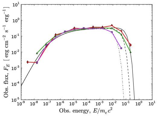
Simulated (coloured) and numerically integrated (black) spectra for a narrow jet observed at different viewing angles. In this plot, Γ₀ = 100, θ_j = 1/Γ₀ and p = 1. Three different viewing angles are shown: θ_v = 0 (0.000 ≤ θ_v ≤ 0.0045, red diamonds and solid black lines); θ_v = θ_j (0.009 ≤ θ_v ≤ 0.011, green triangles and black dashed lines) and θ_v = 2 × θ_j (0.019 ≤ θ_v ≤ 0.020, magenta squares and dot–dashed lines). After viewing angle binning, the red, green and magenta spectra contain 1002, 1758 and 1486 photons, respectively. The photon index below E_peak is α = −1 for all viewing angles, two units less than the Rayleigh–Jeans index. For this parameter space region the numerical integration gives an excellent fit to the simulated spectra.

Figure 7.

Open in new tabDownload slide

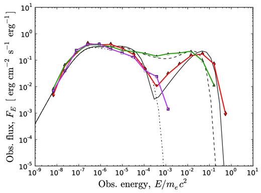
Simulated (coloured) and numerically integrated (black) spectra for narrow jets with different Lorentz factor gradients. In this plot, Γ₀ = 100, θ_j = 1/Γ₀ and θ_v = θ_j (0.009 ≤ θ_v ≤ 0.011). Three different values of p are shown: p = 1 (red diamonds and solid black lines), p = 2 (green triangles and black dashed lines) and p = 4 (magenta squares and dot–dashed lines). After viewing angle binning, the red, green and magenta spectra contain 1758, 1900 and 891 photons, respectively. The low-energy photon index is close to α ≈ −1 for all Lorentz factor gradients considered here. For p = 4, the high-energy spectrum does not decay exponentially due to photon diffusion from high angles. See further discussion in the text.

Figure 8.

Open in new tabDownload slide

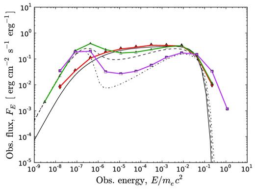
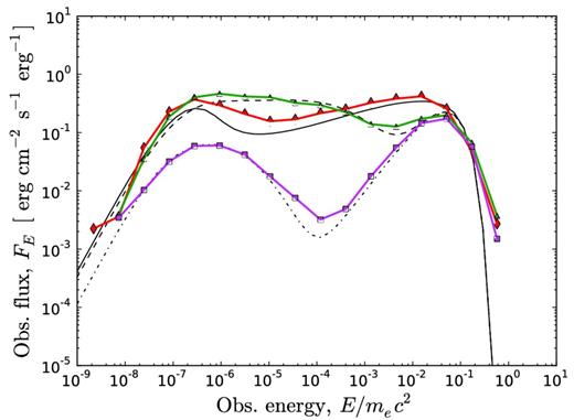
Simulated (coloured) and numerically integrated (black) spectra for a wide jet observed at different viewing angles. In this plot, Γ₀ = 100, θ_j = 10/Γ₀ and p = 4. Three different viewing angles are shown: θ_v = 0 (0.000 ≤ θ_v ≤ 0.006, red diamonds and solid black lines); θ_v = θ_j (0.009 ≤ θ_v ≤ 0.011, green triangles and black dashed lines) and θ_v = 2 × θ_j (0.019 ≤ θ_v ≤ 0.020, magenta squares and dot–dashed lines). After viewing angle binning, the red, green and magenta spectra contain 1577, 1826 and 1112 photons, respectively. For θ_v ≪ θ_j, the high-energy spectrum resembles that of a spherical wind. For θ_v = θ_j, the photon index is α = −1, similar to the spectrum from a narrow jet shown in Fig. 6. Due to the large Lorentz factor gradient (p = 4), for θ_v = 2 × θ_j the peak energy is very low.

Figure 9.

Open in new tabDownload slide

Simulated (coloured) and numerically integrated (black) spectra for jets with different jet opening angles. In this plot, Γ₀ = 100, p = 2 and θ_v = 0 (0.000 ≤ θ_v ≤ 0.006 for the red and green spectra and 0.000 ≤ θ_v ≤ 0.020 for the magenta spectra). Three different values of θ_j are shown: θ_j = 1/Γ₀ (red diamonds and solid black lines), θ_j = 3/Γ₀ (green triangles and black dashed lines) and θ_j = 10/Γ₀ (magenta squares and dot–dashed lines). After viewing angle binning, the red, green and magenta spectra contain 2163, 2267 and 4482 photons, respectively. The exact spectral shape depends on the value of p; however, the average spectral index is approximately −1 for jet opening angles up to |$\theta _{\rm j} \approx \text{few}/\Gamma _{\rm 0}$| and values of p up to a few.

Figure 10.

Open in new tabDownload slide

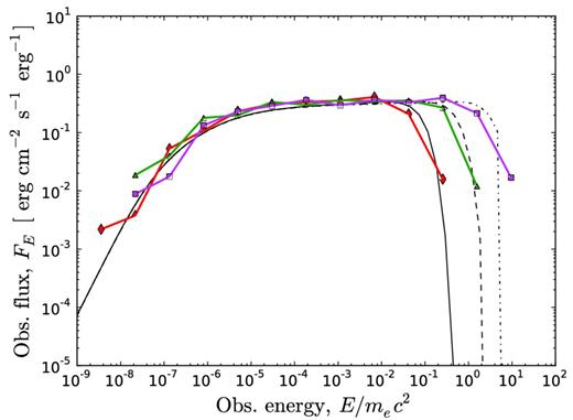
Simulated (coloured) and numerically integrated (black) spectra for narrow jets with different values of Γ₀ but constant values of θ_jΓ₀. In this plot, p = 1, θ_j = 1/Γ₀ and θ_v = 0 (0.000 ≤ θ_v ≤ 0.006 for red, 0.0000 ≤ θ_v ≤ 0.0032 for green and 0.000 ≤ θ_v ≤ 0.0020 for magenta). Three different values of Γ₀ are shown: Γ₀ = 100 (red diamonds and solid black lines), Γ₀ = 200 (green triangles and black dashed lines) and Γ₀ = 400 (magenta squares and dot–dashed lines). After viewing angle binning, the red, green and magenta spectra contain 1934, 558 and 1114 photons, respectively. The magenta spectrum requires small viewing angle bins due to the high Γ₀. Therefore, 1.3 × 10⁸ photons were simulated for the magenta spectrum. For the other two spectra, 1 × 10⁷ photons were simulated. The spectral components from the inner and outer jet regions are shifted to higher energies in accordance with equations (12) and (20).

For a top-hat jet (p → ∞), the most likely viewing angle is θ_v/θ_j ≈ 2/3 since the jet is obscured for θ_v > θ_j. However, the outflows we consider here can be observed at θ_v > θ_j due to the gradual decrease of the Lorentz factor. This increases the value of the most likely viewing angle. A value of θ_v ≈ θ_j may be close to the average value for jets with intermediate values of p (the exact value of the most likely viewing angle depends both on the outflow and detector properties). Therefore, we choose to show θ_v/θ_j = 0, 1 and 2 in Figs 6 and 8.

The most important result of this paper is that we obtain α ≈ −1 (where α is the low-energy photon index in the Band function, dN/dE ∝ E^α below E_peak) for a large region of the considered parameter space. This is demonstrated in Figs 6–10. We consider this a very important result as this is similar to the average low-energy photon index observed in GRBs (e.g. Kaneko et al. 2006; Nava et al. 2011; Goldstein et al. 2012).

For a narrow jet (θ_j = 1/Γ₀; see Fig. 6), the peaks of the emission from the inner and outer jet regions (E_peak and |$E_\mathcal {D}$|⁠, respectively; see discussion in Section 3) coincide, and so the spectrum below E_peak is a pure power law for ∼6 decades in energy. The resulting spectral shape is independent of viewing angle; however, the peak energy decreases as the outflow is observed at large viewing angles.

In Fig. 7 we present spectra for narrow jets with p = 1, 2 and 4 observed at θ_v = θ_j. As can be seen, the low-energy photon index is not very sensitive to the Lorentz factor gradient. The softest spectrum is obtained for p = 1, as shown in Figs 6 and 7. For higher Lorentz factor gradients, there is a slight increase in the photon index, consistent with the analytical expression in equation (26). For 1 < p < 4, the photon index is −1 ≲ α ≲ −0.5. Values of p lower than unity have been considered. As p decreases below unity, the photon index below the peak energy increases. For p = 0, the outflow profile is spherically symmetric. Therefore, the observed spectrum is that of a spherically symmetric wind (α ≈ 0.4).¹² For the simulated spectra, the exponential cut-off expected at energies above the peak energy becomes less sharp for increasing values of p. We discuss this further below.

The spectra from jets with large opening angles (θ_j ≈ 10/Γ₀) observed at θ_v ≪ θ_j appear as those from spherically symmetric winds. However, for viewing angles θ_v ≈ θ_j the observed photon index below the peak energy is lower. In Fig. 8 we present spectra from an outflow with the profile Γ₀ = 100, θ_j = 0.1 and p = 4 observed at different viewing angles. For θ_v = θ_j, α ≈ −1, just as for narrow jets. Due to the large Lorentz factor gradient, E_peak decreases rapidly with increasing viewing angle. In Fig. 8, E_peak(θ_v = 2 × θ_j)/E_peak(θ_v = 0) ≈ 10⁻³. As discussed above, depending on the jet properties and detector characteristics, the most likely viewing angle may be close to the jet opening angle.

In Fig. 9 we present observed spectra from jets with different opening angles (θ_jΓ₀ = 1, 3 and 10) viewed head-on. Both θ_jΓ₀ = 1 and 3 result in low-energy slopes close to α = −1, independent of viewing angle, while wider jets viewed at θ_v = 0 result in a spherically symmetric spectral shape a few decades below E_peak.

Increasing the maximum Lorentz factor, Γ₀, shifts the spectral components from the inner and outer jet up in energy while keeping their spectral shapes intact [Fig. 10; also see equations (12), (13), (20) and (23)]. The envelope component is unaffected (as expected; see equation 27). As long as Γ₀θ_j is constant, the spectral shapes of the inner and outer jet components are not affected by varying Γ₀.

We reach the conclusion that the low-energy spectral index is close to α ≈ −1 for narrow jets, with |$\theta _{\rm j} \le \text{few}/\Gamma _{\rm 0}$| and moderate Lorentz factor gradients for all viewing angles. Similar photon indices are obtained from wider jets observed at θ_v ≈ θ_j.

5.1 Asymmetric photon diffusion and Comptonization

Preferential photon diffusion towards the jet centre is expected to occur in outflows where the bulk Lorentz factor decreases from the jet axis. This can be understood in terms of average photon scattering angles. The average photon scattering angle with respect to the radial direction is ∼1/Γ in the lab frame. Therefore, a photon is more likely to scatter from a region of low Lorentz factor to a region of high Lorentz factor than the other way around. The importance of photon diffusion is dependent on the Lorentz factor gradient, and so the spectra from jet profiles with large values of p are expected to differ from the numerically integrated spectra where we assume |${\rm d}\dot{N}_\gamma /{\rm d}\Omega$| is r-independent. This is indeed observed in the simulations. The effects of angular photon diffusion are, however, subdominant as compared to the observed temperature variations across the jet when considering the formation of the observed spectrum from jets with small Lorentz factor gradients (approximately p ≲ 4).

Comptonization of photons propagating to regions of higher Lorentz factor may cause photons to fall out of thermal equilibrium with the local electrons. This has been investigated by comparing the simulated lab frame photon energy to the lab frame temperature of the electrons at the last scattering position for all photons in a given spectrum. The observed photon energies are well described by the local observed temperature for most of the considered parameter space. However, a deviation is observed in Figs 7 and 11. The expected high-energy cut-off is significantly smoother for the spectrum with p = 4 observed at θ_v = θ_j. The same jet observed at θ_v = 0 forms a high-energy power law with photon index β ≈ −2. The photons forming the power law start out with thermal energies in the outer jet region where the Lorentz factor gradient is large. Repeated scatterings towards the jet centre increase the photon energy until the photon reaches the inner jet region where it finally escapes. The final photon temperature depends on the initial thermal photon energy, the number of scatterings before escape and the average energy gained in each scattering. The last two terms are dependent on the Lorentz factor gradient. The Comptonization of photons propagating in media with a Lorentz factor gradient will be further explored in future works. In general, the analytical expressions for characteristic energies and spectral shapes presented in Section 3 agree well with the Monte Carlo simulations except for large Lorentz factor gradients.

Figure 11.

Open in new tabDownload slide

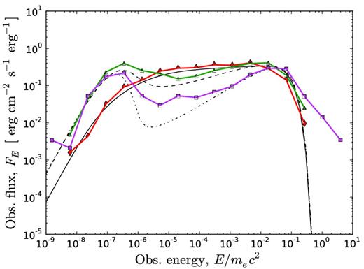
Same as Fig. 7, but θ_v = 0 (0.000 ≤ θ_v ≤ 0.006). After viewing angle binning, the red, green and magenta spectra contain 1934, 2166 and 1178 photons, respectively. A power law above the peak energy is seen in the magenta spectrum. The power law is further discussed in the text.

6 DISCUSSION

6.1 Sensitivity to the chosen dynamics and Lorentz factor profile

In this work we consider fireball dynamics for the outflow properties. However, other dynamics are possible: kinetic energy dissipation may be significant during the acceleration phase or the outflow may be dominated by magnetic fields. The overall shape of the spectral components from the inner jet and envelope regions is not expected to be sensitive to the exact dynamics; however, the value of E_peak is dependent on the radial scalings of the outflow properties. The exact value of the power-law slope in the outer jet component is expected to be modified for other dynamics, as well as |$E_\mathcal {D}$| (equation 20) (the energy of the spectral bump below the peak energy in Fig. 3). However, the ratio E_j/E_peak which gives an indication of the energy where the spectrum starts to deviate from the spherically symmetric spectrum is not sensitive to the dynamics.

The shape of the angular profile is motivated by hydrodynamical simulations. One may consider other shapes (e.g. Gaussian) for the angular parameters. The exact values of the characteristic energies and spectral shapes are naturally dependent on the chosen profile; however, the general spectral features are not sensitive as long as the considered profile has similar characteristics.

6.2 Relative photon time delays

In this work we focus on the spectrum from steady jets. In much the same way as photons from a certain angle have a characteristic energy, they also have a characteristic time delay as compared to a photon from the centre of the jet. One can therefore associate a given photon energy in the spectrum with a certain time delay.

This result may be compared to the case of an angle-independent emission radius (such as the case for the afterglow; e.g. Kumar & Panaitescu 2000). Assuming the emission radius to be equal to the photospheric radius at the LOS, photons with energy E = 10⁻² E_peak (originating at θ > 1/Γ) arrives with a time delay of Δt^ob ≈ 4 × 10⁻³(L/10⁵²)(Γ/300)⁻⁵([E/E_peak]/10⁻²)⁻¹ s. This time delay is three orders of magnitude shorter than the result obtained in equation (29). This example highlights the importance of recognizing the angular dependence of the photospheric radius.

The spectral component associated with the envelope has a very long associated time delay, due to the large photospheric radius (see Fig. 5). We therefore do not expect the envelope component to be observed in the prompt emission emitted from a transient source.

6.3 Band-like GRB spectra

Observed GRB spectra do not, in general, appear thermal. The spectra are usually well fitted by the Band function, although more complex spectra have been observed (e.g. Ryde et al. 2010; Ackermann et al. 2011; Guiriec et al. 2011). The average values of the low- and high-energy photon indices are α ≈ −1 and β ≈ −2.5, respectively. This is in contrast to a blackbody spectrum in which α = 1, and the spectrum cuts off exponentially above the peak energy. To reconcile the photospheric model with observations, energy dissipation close to the photosphere has been considered as a way to modify the local comoving photon spectrum (Thompson 1994; Spruit et al. 2001; Giannios & Spruit 2005; Pe'er et al. 2005, 2006; Rees & Mészáros 2005; Lazzati et al. 2009; Beloborodov 2010; Ryde et al. 2011; Vurm et al. 2011; Zhang & Yan 2011). In these scenarios, the observed spectrum results from a combination of radiative processes. Comptonization of the thermal photon spectrum is the source of the high-energy power law, and synchrotron photons contribute to the low-energy spectrum (e.g. Vurm et al. 2011). In this work we show that 3D effects arising from the jet shape may add a significant contribution to understanding the soft low-energy spectrum. Narrow jets or wider jets observed at θ_v ≈ θ_j result in a low-energy photon index α ≈ −1 under natural assumptions. Harder values of the low-energy photon index are obtained for wide jets viewed at θ_v ≪ θ_j. The details of the observed spectrum predicted here are expected to be modified if significant energy dissipation takes place below the photosphere, since in this scenario the outflow dynamics is changed. Moreover, as discussed above, in such a scenario the soft tail of the spectrum may be modified by non-thermal emission.

In some GRBs observed by the Fermi Gamma-Ray Space Telescope [GRB 100724B Guiriec et al. (2011) and GRB 110721A Axelsson et al. (2012)], a spectral ‘bump’ is significantly detected at energies below the main peak. This bump is commonly interpreted as photospheric emission (e.g. Ryde 2005). In such a scenario, the Band component originates from non-thermal emission processes in the optically thin part of the outflow outside the photosphere (e.g. Veres, Zhang & Mészáros 2012; Zhang et al. 2012). Within this interpretation the analysis performed in this paper is applicable to the bump instead of the Band component and may explain bumps wider than blackbody.

7 SUMMARY AND CONCLUSIONS

In this work we develop the theory of photospheric emission from relativistic jets with angle-dependent outflow properties. We consider a three-parameter angular Lorentz factor profile (equation 1) where the Lorentz factor is approximately constant, Γ = Γ₀, within a characteristic jet opening angle θ_j and then decreasing approximately as Γ ∝ θ^−p towards the outer jet edge. The shape of the profile is motivated by the results of hydrodynamical simulations of jet propagation through the progenitor star (e.g. Aloy et al. 2000; Zhang et al. 2003; Morsony et al. 2007; Mizuta et al. 2011). In Section 2 the expression for the observed spectrum is obtained analytically by integrating the local emissivity over all radii and angles (equation 10). We derive approximate analytical expressions for the important spectral features in Section 3. Comparing jetted outflows to spherical outflows, we show that softening of the spectrum below the peak energy is expected for an on-axis observer. This is a consequence of weaker radial beaming of photons at high latitudes due to the decreasing Lorentz factor. A Monte Carlo simulation was developed to investigate the importance of full photon propagation below the photosphere (Section 4). In Section 5 we present spectra obtained by numerical integration of equation (10) as well as the Monte Carlo simulations for different profile parameters and viewing angles (Figs 6–11).

The most important result of this paper is that the photospheric spectrum below the thermal peak may be significantly softer than blackbody, as a consequence of geometrical broadening. In particular, we obtain a photon index α ≈ −1 below the peak energy for a large region of the considered parameter space. For narrow jets (⁠|$\theta _{\rm j} \lesssim \text{few}/\Gamma _{\rm 0}$|⁠) with Lorentz factor gradients 1 ≤ p ≤ 4 observed at any viewing angle, we find −1 ≳ α ≳ −0.5. For jets with θ_j ≈ 1/Γ₀ and p ≥ 1, α ≈ −(1/4)(1 + 3/p) (see equation 26). Observing wider jets (θ_j ≳ 5/Γ₀) at θ_v ≈ θ_j results in similar soft spectra with α ≈ −1. However, spectra from wide jets observed at small angles (θ_v ≪ θ_j) appear similar to the spectrum from a spherical wind (i.e. close to blackbody but with α ≈ 0.4 at E = 10⁻² E_peak) for several decades below the peak energy. This may explain the hard low-energy photon indices observed in some GRBs [α ≈ 0 (Goldstein et al. 2012); see further discussion below]. However, observing the outflow at viewing angles θ_v ≈ 0 is less likely than θ_v ≈ θ_j. Additionally, increasing the viewing angle causes the observed peak energy to decrease. The decrease is slower for low Lorentz factor gradients. Therefore, such outflows may still be observed at |$\theta _{\rm v} \approx \text{few} \times \theta _{\rm j}$|⁠.

Photon diffusion primarily towards regions of higher Lorentz factor is observed in the simulations. For outflows with large Lorentz factor gradient (p ≳ 4), this bulk propagation of photons has to be taken into account when computing the observed spectrum. Comptonization of the photons that make repeated scatterings towards regions of larger Lorentz factor can produce photons with energies significantly higher than the local temperature. Evidence for this can be seen in Fig. 11 (p = 4), where an approximate high-energy power law is formed above the peak energy. Photon propagation in plasma with a steep Lorentz factor gradient will be further explored in future works.

The observed photospheric spectrum from a spherical outflow has previously been considered in the literature (e.g. Beloborodov 2010; Pe'er & Ryde 2011). In the limiting case of outflows with θ_j ≳ 5/Γ₀ observed at θ_v ≪ θ_j, we obtain similar results. For larger viewing angles or smaller jet opening angles, geometrical broadening of the spectrum has to be considered.

Although we consider a static source, as shown in Section 6.2 there is a time delay associated with high-latitude photons. The time delay increases with decreasing observed photon energy. The time delay at a specific energy is longer for more narrowly collimated jets. For a narrow jet (θ_j = 1/Γ₀) with typical outflow parameters characterizing GRBs, the time delay is ≈1 s at E ≈ 10⁻²E_peak. Spectral analysis of prompt GRB emission using smaller time bins than this time delay may reveal harder spectra within the energy range 10⁻²E_peak ≲ E ≲ E_peak than what is predicted by the static model.

For this work we have considered outflows with angle-independent luminosity, and so the shape of the Lorentz factor profile is fully determined by the angle-dependent baryon loading. As shown above, the spectral slope in the range 10⁻²E_peak ≲ E ≲ E_peak is formed by photons making their last scattering at θ ≲ 5/Γ₀. Therefore, this assumption is a good approximation for jets where |${\rm d}L/{\rm d}\Omega \approx \text{const}$| for θ ≲ 5/Γ₀. This requirement is fulfilled for model JA in Zhang et al. (2003) close to the largest radius of the simulation (r = 2.1 × 10¹⁰ cm). In our notation, Γ₀ ≈ 140, θ_j ≈ 0.017 ≈ 2.5/Γ₀ and p ≈ 6.5 for model JA, as estimated from figs 8 and 9 in Zhang et al. (2003).

Furthermore, we consider non-dissipative fireball dynamics. The dynamics of the outflow are dependent on the dominant form of energy carried by the jet as well as energy dissipation. In particular, the radial scalings of the comoving temperature and Lorentz factor in magnetically dominated outflows are expected to differ significantly from the scalings of thermal fireballs. Giannios (2012) and Beloborodov (2012) considered the scaling of E_peak in dissipative outflows. Heating keeps the comoving temperature approximately constant in the range R_ph/30 ≲ r ≲ R_ph, in contrast to the non-dissipative outflows considered here. However, the framework presented in Section 2 is general and may be applied to any relativistic, optically thick outflow.

Since the causally connected parts of the outflow are separated by angles ≈1/Γ, one may consider outflows with Lorentz factor variations at angular scales of |$\Delta \theta \approx \text{few}/\Gamma$|⁠. Geometrical broadening of the observed spectrum is expected as a consequence of the beaming of photons being a function of angle from the jet axis, in much the same way as for the jets considered in this work. The spectral slope below the peak energy is expected to depend on both the typical angular scale and the amplitude of the Lorentz factor variations.

Spectral broadening by energy dissipation in regions of moderate optical depth may be combined with geometrical broadening. As the observed spectrum below the peak energy is a superposition of comoving spectra, it is not sensitive to the exact shape of the comoving spectrum. Comptonization of the comoving spectrum by electrons which are heated by energy dissipation (e.g. Beloborodov 2010; Lazzati & Begelman 2010) can shape the spectrum above the peak energy, while geometrical broadening forms the spectrum below the peak energy.

The observed low-energy photon index varies between bursts, forming an approximately Gaussian distribution centred at α ≈ −1 with a full width at half-maximum of ≈1 (e.g. Goldstein et al. 2012). Within the framework presented in this paper, the distribution could naturally be interpreted as a result of viewing angle variations. In particular, observing a wide jet at zero viewing angle results in α ≈ 0.4. The exact α-distribution predicted by our model is hard to obtain, since it depends on detector characteristics. However, a clear prediction of the model is that of softening of the low-energy photon index with increasing viewing angle for jets with θ_j ≳ few/Γ₀.

GRB 090902B is a burst of special interest, due to its unusual spectral shape (Abdo et al. 2009). The prompt spectrum consists of a sharply peaked Band component along with a wide power law. The hard low-energy photon index and the narrow width of the Band component pose an extreme challenge for optically thin emission models. Therefore, a photospheric origin of the Band component in this burst seems inevitable (Ryde et al. 2010, 2011; Zhang et al. 2011; Pe'er et al. 2012). Since the Band component appears close to blackbody, processes that are expected to modify the photospheric spectrum can be constrained for GRB 090902B. The rate of energy dissipation in regions of moderate optical depth must be relatively low as the observed Band component is not severely distorted from the Planck spectrum. Within the framework considered in this paper, further constraints can be set. The requirement for geometrical broadening to not significantly distort the observed spectrum in the energy range 10⁻²E_peak ≲ E ≲ E_peak is θ_v ≪ θ_j and θ_j ≳ 5/Γ₀. Depending on typical GRB outflow characteristics, the probability for such parameter combinations may be low. This would help explain the rarity of similar events.

Multiple spectral components have been clearly identified in several GRBs after the launch of the Fermi telescope (Abdo et al. 2009; Ackermann et al. 2010, 2011). This was expected from a theoretical point of view, simply because of the wide energy range of the observations. Several models predict non-thermal spectral components as a result of kinetic or magnetic energy dissipation above the photosphere (e.g. Mészáros et al. 2002; Zhang & Yan 2011). If dissipation occurs at r ≫ R_ph, the thermal and non-thermal components may be fitted separately (such as in 090902B, Pe'er et al. 2012). For dissipation at r ≳ R_ph, the separation of thermal and non-thermal components may be less clear because of the coupling of the thermal photon field to the accelerated non-thermal electrons. In this work we consider the thermal component in isolation in order to demonstrate the geometrical broadening of the spectrum. However, a complete theory for the prompt GRB emission must explain all observed spectral components.

An outstanding problem for the photospheric interpretation of prompt GRB emission is the non-thermal spectra commonly observed. In particular, the average low-energy photon index is not compatible with the Rayleigh–Jeans index (α ≈ −1 as compared to α = 1). In this work we show that either a narrow jet (⁠|$\theta _{\rm j} \lesssim \text{few} / \Gamma _{\rm 0}$|⁠) with a moderate Lorentz factor gradient (1 ≤ p ≤ 4) observed at any viewing angle or a wide jet observed at θ_v ≈ θ_j can naturally produce −1 ≲ α ≲ −0.5 through geometrical broadening, without a need for additional emission processes such as synchrotron emission to supply photons below the thermal peak.

We would like to thank Peter Mészáros, Martin Rees and Bing Zhang for useful discussions. The Swedish National Space Board is acknowledged for financial support. AP wishes to acknowledge support from Fermi GI programme #41162.

REFERENCES