


Few studies have reported on the fine-scale population genetics of batoid species in the Atlantic basin. Here, we investigate the genetic diversity and population structure of the spotted eagle ray, Aetobatus narinari, sampled in the northeastern and southwestern parts of the Gulf of Mexico and in the northwestern Caribbean Sea. Samples were collected from 286 individuals sampled across 3 geographic localities. Estimates of divergence based on the mitochondrial cytochrome b gene and 10 nuclear microsatellite loci reveal weak but significant genetic structure among A. narinari populations in this region. Analysis of molecular variance estimates based on both marker types indicate significant differentiation between Florida and Mexico populations, while comparisons with Cuba suggest high levels of gene flow with rays from both Mexico and Florida. Conflicting results were found from the different marker types when sexes were analyzed separately underscoring the importance of applying multiple marker types when making inferences about population structure and sex-biased dispersal. Results from Bayesian clustering analyses suggest rays may be migrating south out of the Gulf of Mexico and into the northwestern Caribbean Sea. Given the impacts of fisheries on this species, coupled with the lack of population genetic data available, these findings offer valuable information to aid with conservation management strategies.
Over the last decade, the scientific community has paid considerable attention to the conservation of elasmobranchs. The combined effects of increased fishing pressures, habitat degradation, and climate change have caused the decline of many shark and ray species (Stevens et al. 2000; Shepherd and Myers 2005; Chin et al. 2010; Simpfendorfer et al. 2011; Dulvy et al. 2014; Randhawa et al. 2014) alarming scientists and conservation managers alike. As long-lived, late maturing animals with low fecundities, elasmobranchs are more susceptible to fishing impacts compared with many other marine species (Stevens et al. 2000). The spotted eagle ray, Aetobatus narinari, is a large marine batoid found circumglobally in tropical and warm-temperate waters (Bigelow and Schroeder 1953; Last and Stevens 1994). This live-bearing species gives birth to between 1 and 4 pups per year (Bigelow and Schroeder 1953; Kyne et al. 2006). As highly mobile rays, A. narinari typically travel in the water column over sandflats and in tidal lagoons while diving to consume benthic prey (Silliman and Gruber 1999; Ajemian et al. 2012; Bassos-Hull et al. 2014). Both single individuals and mixed-sex aggregations have been documented, and tag-recapture and satellite data indicate multiyear site fidelity, short and long-distance movement patterns, and seasonal abundance trends (Corcoran and Gruber 1999; Ajemian et al. 2012; Bassos-Hull et al. 2014; Ajemian and Powers 2014; Hueter R, unpublished data). The vulnerability of this species to both targeted and nontargeted fisheries has been reported (Devadoss 1984; Trent et al. 1997; Dubick 2000; Shepherd and Myers 2005; Cuevas-Zimbrón et al. 2011; Tagliafico et al. 2012) and underscores the importance of studying the effects of these takes on its genetic diversity and population structure. In addition, recent molecular and morphological evidence suggest taxonomic revision of the genus Aetobatus is warranted (CytB, COI, ITS2—Richards et al. 2009; NADH2—White et al. 2010, 2013; Naylor et al. 2012; White and Moore 2013; White 2014). As additional data become available, the geographic distributions of these species will be further resolved.
Within batoids, the few studies published on population genetics report evidence of both fine-scale structure and lack of structure among coastal populations. Schluessel et al. (2010) found a surprising amount of genetic structure among populations of A. narinari within the Indo-Pacific based on 2 mitochondrial DNA (mtDNA) markers, Cytb and NADH4, whereas Newby et al. (2014) found no genetic structure among A. narinari populations sampled off the southeastern United States using nuclear microsatellite data. Although these 2 studies are the only other population genetic studies published on eagle rays, population-level studies have been conducted on near relatives using various mitochondrial loci. For example, within the Gulf of California, as well as along the Pacific coast of Baja California, Mexico, populations of Rhinoptera steindachneri are not genetically distinct, but genetic divergence of populations between these 2 areas is high (NADH2—Sandoval-Castillo and Rocha-Olivares 2011). This is also the case for populations of Gymnura marmorata, where significant genetic structure exists between the Gulf of California and Pacific coast of the Baja California peninsula, with little structure found among coastal samples (Cytb—Smith et al. 2009). Although Dasyatis brevicaudata shows the trend of high divergence across ocean basins, this species also shows significant genetic differentiation among coastal New Zealand populations (mtCR—Le Port and Lavery 2012).
From these and other studies, it is apparent that aspects of batoid biology—such as movement patterns, genetic discreteness, and habitat preference—are varied and not predictable based on just 1 characteristic, such as vagility of that species. One general trend, also proposed for shark species, is that of coastal connectivity of populations with structure occurring across ocean basins. There is some evidence to support this trend in A. narinari as samples taken from coastal sites along Florida, Georgia, and South Carolina show no genetic structure based on microsatellite data (Newby et al. 2014). Although Schluessel et al. (2010) found very high levels of genetic differentiation in A. narinari on a regional scale, analyses were not done on a finer scale due to limited sample sizes. Within the Gulf of Mexico, the population genetic structure of A. narinari is unknown and has not yet been investigated on a fine scale.
To date, elasmobranch population genetic studies reporting on areas in the Gulf of Mexico have focused on shark species and have shown both significant and nonsignificant structure among areas within this ocean basin. For example, Heist et al. (1995) showed Carcharhinus plumbeus found in the Gulf of Mexico and western North Atlantic form 1 panmictic population. Based on mtDNA control region sequence data, Keeney et al. (2003) did not find significant structure among Carcharhinus limbatus sampled from 3 Florida nurseries. However, a follow-up study using both mtDNA and microsatellite data did detect significant heterogeneity among C. limbatus of eastern Gulf, western Gulf, and northern Yucatan regions using both marker types (Keeney et al. 2005). Using microsatellite data from 4 polymorphic loci, Feldheim et al. (2001) concluded weak genetic structure exists between Negaprion brevirostris from Gulf of Mexico and Caribbean sites. Recently, Portnoy et al. (2014) documented significant heterogeneity among populations of Carcharhinus acronotus in the Gulf based on both mtDNA control region sequence and nuclear microsatellite data. Thus far, there are no published studies reporting on the genetic population structure of any batoid species in the Gulf of Mexico.
Here, we investigate the genetic diversity and population structure of A. narinari sampled in both the northeastern and southwestern parts of the Gulf of Mexico and northwestern Caribbean Sea. The questions we address are 1) does heterogeneity exist among populations of A. narinari sampled off Florida, Mexico, and Cuba? 2) if heterogeneity does exist, is it equal among sexes or is there evidence for sex-biased dispersal? and 3) do genetic data support seasonal migration patterns as suggested by photo-identification studies of this species?
Materials and Methods
Study Sites and Sampling
We collected 171 pelvic fin clips from A. narinari in Sarasota Bay, Florida (FLA), between 2009 and 2011 (Figure 1). The majority of these samples (92%) were collected during the months of April–November, when rays are most abundant in this area (Bassos-Hull et al. 2014). A detailed account of field methods for the Florida samples is reported in Bassos-Hull et al. 2014. Samples collected off Mexico (MEX) totaled 96 and were obtained from target fisheries off Isla Arena (n = 19), Campeche (n = 10), Seybaplaya (n = 34), Champoton (n = 16), Sabancuy (n = 2), and Tabasco (n = 8) in 2009, 2011, and 2013 (Figure 1). For 7 Mexico samples, collection locality was recorded as either Champoton or Seybaplaya. The majority of Mexico samples (70%) were collected during the months of November–April when rays are more abundant in the southern Gulf of Mexico (Cuevas-Zimbrón et al. 2011). As initial tests of population differentiation among these localities revealed no structure, all Mexican samples were pooled and treated as 1 population in further analyses. Finally, 19 samples were collected on 14 February 2013, from a target fishery off the southwestern coast of Cuba, in the Ensenada de la Siguanea, on the western side of Isla de la Juventud. At all sampling localities, sex was determined by the presence or absence of claspers as described in Bassos-Hull et al. (2014).
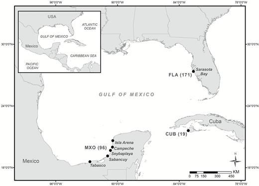
Map of Aetobatus narinari sampling localities with sample size noted in parentheses. Sarasota Bay, Florida (FLA), Mexico (MXO), and Cuba (CUB).
Genetic Techniques
Genomic DNA was extracted from approximately 25mg of tissue using Qiagen DNeasy Blood and Tissue kits following the manufacturer’s protocol (Qiagen). The quality and concentration of extractions were then assessed using a Nanodrop 2000c spectrophotometer, and all samples were diluted to a working concentration of 20ng/μL for further steps. All samples were genotyped for 10 polymorphic microsatellite loci developed from A. narinari. Primers used and PCR conditions for these markers are outlined in Sellas et al. (2011). Fragment analysis was carried out on an ABI3130xl Genetic Analyzer (Applied Biosystems) using the GSLIZ600 size standard, and genotypes were scored using GeneMapper v. 4.0 (Applied Biosystems). The program MICROCHECKER (van Oosterhout et al. 2004) was used to test for allelic dropout and the presence of null alleles. Exact tests for Hardy–Weinberg equilibrium (HWE) were carried out using GENEPOP (Raymond and Roussett 1995). Observed and expected heterozygosities and tests for departure from linkage equilibrium were conducted using ARLEQUIN v. 3.5 (Schneider et al. 2000). Estimates of allelic richness were obtained using FSTAT v. 2.9.3.2 (Goudet 1995). The Microsoft Excel add-in GenAlEx v. 6.5 (Peakall and Smouse 2006) was used to identify duplicate genotypes in the data set. In such cases, one of the duplicate samples was removed from further analyses. In order to ensure a high number of related individuals were not influencing our population structure measures, estimates of relatedness (Queller and Goodnight 1989) were obtained for each population using GenAlEx v. 6.5. Average relatedness estimates per population as well as pairwise relatedness values were obtained. From these, the percent of each sample representing unrelated (R < 0), average related (0 < R < 0.2), half sib related (0.2 < R < 0.4), and full sib/parent–offspring related (0.4 < R < 0.6) levels were recorded and compared across populations. Wright’s FST estimates were obtained by running an analysis of molecular variance (AMOVA) using ARLEQUIN with significance tested against 10 000 permutations. The AMOVA significance level was adjusted to α = 0.016 based on Bonferroni correction for 3 simultaneous comparisons (Rice 1989). AMOVA’s were also carried out for male and female samples separately to investigate the possibility of sex-biased dispersal. The number of discrete populations present in the overall sample was calculated using the program STRUCTURE (Pritchard et al. 2000). STRUCTURE was run 10 independent times under the admixture model with correlated allele frequencies for 100 000 steps after 50 000 initial burn-in steps testing K values 1–10. The use of sample location information was allowed to inform cluster assignments as recommended for data sets with low information content (Hubisz et al. 2009). The web-based program STRUCTURE HARVESTER (Earl and vonHoldt 2012) was then used to assess likelihood values and determine the K value that best fits the data based on the method of Evanno et al. (2005). To identify first-generation migrants, we used the Lhome likelihood test statistic of the program GENECLASS 2.0 (Piry et al. 2004). We chose this statistic based on the suggestion of Piry et al. (2004) to do so in cases where all source populations have not been sampled. The Bayesian criterion of Rannala and Mountain (1997) was selected along with the resampling method of Paetkau et al. (2004). We ran 100 000 simulations with α = 0.05. Estimates of historical gene flow were calculated for the 10 microsatellite loci using MIGRATE-N 3.5.1 (Beerli and Felsenstein 2001; Beerli 2006), using a Bayesian coalescent-based framework. The full migration model was used to estimate the migration rates between the 3 localities, with 1 long chain of 5000 genealogies recorded at a sampling increment of 200 and a burn-in of 10 000. The analysis was repeated 10 times with different uniform priors of θ and M (upper boundaries of 1–100 for θ and 100–1000 for M), in order to estimate the most appropriate boundaries. The results presented were estimated with a uniform prior of 0–8 for θ and 0–1000 for M. All the estimates obtained had an effective sample size greater than 1000.
A 580-bp fragment of the mitochondrial cytochrome b gene was amplified via PCR and sequenced using the primers AnarCBF1 (5′-GAGGGGCAACTGTCATCACTAACC-3′) and AnarCBR1 (5′-CGATTGGGAAAAGGAGGAGGAA-3′) from Richards et al. (2009). PCR reactions (25 μL) consisted of 1× PCR buffer (10mM Tris–HCl, 1.5mM MgCl2, 50mM KCl, pH 8.3), 1.0 μM of each primer, 400 μM each dNTP, 1.0U of Taq, and 20ng of genomic DNA. The thermal cycling profile was as follows: initial denaturation at 94 °C for 3min, followed by 35 cycles of 94 °C for 30 s, 53 °C for 30 s, and 72 °C for 45 s. PCR products were purified using the ExoSAP-IT enzyme mix (USB) and sequenced in both directions using BigDye Terminator v. 3.1 (Applied Biosystems). Following a standard ethanol precipitation clean-up step (Sambrook et al. 1989), products were sequenced on an ABI3130xl Genetic Analyzer (Applied Biosystems). Sequence editing and alignment were carried out using the program Geneious v. 5.64. Shared and unique haplotypes were identified using MacClade v. 4.08 (Maddison and Maddison 2000). Nucleotide (π) and haplotype (h) diversities were estimated for each population using ARLEQUIN. To measure the degree of population subdivision, an AMOVA was run using ARLEQUIN applying the Kimura 2-parameter model of sequence evolution (Kimura 1980).
In compliance with data archiving guidelines (Baker 2013), we have deposited the primary data sets underlying these analyses with Dryad (doi:10.5061/dryad.n914n).
Results
Genetic Diversity
From the microsatellite loci, the average number of alleles per locus ranged from 2 to 27 with both the lowest and highest numbers found in the Mexico sample. Average observed heterozygosity estimates were relatively uniform across populations (0.713 in the Florida sample, 0.718 in the Mexico sample, and 0.747 in the Cuba sample; Table 1). None of the 10 microsatellite loci deviated significantly from HWE, whereas 2 loci (SER44 and SER61) showed evidence of linkage disequilibrium in the Mexico population after Bonferroni correction. Removal of these loci did not change significance of final results. Results from MICROCHECKER showed no significant evidence of scoring error, allelic dropout, or null alleles for any of the microsatellite loci. Two pairs of individuals in the Florida sample had identical genotypes across all loci and were assumed to be re-samples of the same individual; therefore, 1 sample from each of these pairs was removed from further analyses. Average relatedness estimates were similar across populations (Table 1). When broken down by range in relatedness values, samples from Florida and Mexico contained comparable proportions of unrelated, average, moderate, and highly related individuals, whereas almost all of the Cuba samples (98%) fell in the average category (R values between 0.00 and 0.20; Table 2).
Genetic diversity and relatedness estimates for Aetobatus narinari sampling localities including sample size (N), number of alleles (A), allelic richness (Rs), observed heterozygosity (Ho), expected heterozygosity (He), average relatedness (R), number of haplotypes (H), haplotype diversity (h), and nucleotide diversity (π)
| N | A | Rs | Ho | He | R | H | h | π | |
|---|---|---|---|---|---|---|---|---|---|
| FLA | 169 | 13.1 | 9.74 | 0.713 | 0.727 | –0.007 | 9 | 0.710 ± 0.03 | 0.0024 |
| MXO | 96 | 15.5 | 9.27 | 0.718 | 0.726 | –0.018 | 5 | 0.536 ± 0.05 | 0.0022 |
| CUB | 19 | 9.9 | 9.90 | 0.747 | 0.764 | –0.056 | 3 | 0.561 ± 0.10 | 0.0024 |
Percentage of pairwise relatedness values for each relatedness category estimated per locality
| Category (R-value) | FLA | MXO | CUB |
|---|---|---|---|
| Unrelated (R < 0) | 53.3 | 54.7 | 2.4 |
| Average (R = 0.00 − 0.20) | 37.5 | 36.1 | 97.6 |
| Half sib (R = 0.21 − 0.40) | 8.6 | 8.8 | 0.0 |
| Full sib, parent/offspring (R = 0.41 − 0.60) | 0.6 | 0.4 | 0.0 |
| Category (R-value) | FLA | MXO | CUB |
|---|---|---|---|
| Unrelated (R < 0) | 53.3 | 54.7 | 2.4 |
| Average (R = 0.00 − 0.20) | 37.5 | 36.1 | 97.6 |
| Half sib (R = 0.21 − 0.40) | 8.6 | 8.8 | 0.0 |
| Full sib, parent/offspring (R = 0.41 − 0.60) | 0.6 | 0.4 | 0.0 |
From the mtDNA data, 9 variable sites defined a total of 10 unique haplotypes (Table 3). Nine haplotypes were found in the Florida population, 5 in the Mexico population, and 3 in Cuba (Table 3). The 3 most common haplotypes in each sample were also previously reported by both Richards et al. (2009) and Schluessel et al. (2010). Number of haplotypes and haplotype and nucleotide diversities per sampling locality are listed in Table 1 with haplotype frequency information listed in Table 3. All 10 unique cytochrome b haplotype sequences were deposited to GENBANK under accession numbers KJ814012–KJ814021.
Haplotype frequency listed per sampling locality along with polymorphic nucleotide position and base information. Nucleotides identical to haplotype 1 are noted with” . ”
| Haplotype | FLA | MXO | CUB | Nucleotide position | ||||||||
|---|---|---|---|---|---|---|---|---|---|---|---|---|
| 21 | 107 | 118 | 141 | 192 | 273 | 321 | 417 | 522 | ||||
| H1 | 27 | 6 | 0 | G | T | T | C | C | A | C | C | C |
| H2 | 80 | 61 | 12 | A | . | . | . | . | . | . | . | . |
| H3 | 27 | 22 | 3 | . | . | . | . | . | . | T | . | T |
| H4 | 8 | 0 | 0 | . | . | . | . | T | . | . | . | . |
| H5 | 22 | 6 | 4 | . | . | . | T | . | . | . | . | . |
| H6 | 2 | 0 | 0 | A | C | . | . | . | . | . | . | . |
| H7 | 1 | 0 | 0 | . | . | . | . | . | G | . | . | . |
| H8 | 1 | 0 | 0 | . | . | C | . | T | . | . | . | . |
| H9 | 1 | 0 | 0 | . | . | . | . | . | G | . | T | . |
| H10 | 0 | 1 | 0 | . | . | . | . | . | . | T | . | . |
Population Differentiation
Based on the microsatellite data, AMOVA analysis revealed weak but significant structure between A. narinari populations in Florida and Mexico (FST = 0.004, P = 0.013) with nonsignificant structure found between Florida and Cuba (FST = 0.002, P = 0.224) and Mexico and Cuba localities (FST = 0.002, P = 0.237; Table 4). AMOVA results based on the mtDNA sequence data also detected significant structure between the Florida and Mexico populations (ΦST = 0.020, P = 0.015), but no structure between Cuba and Florida (ΦST = –0.007, P = 0.528) or Mexico and Cuba (ΦST = –0.007, P = 0.461). When sexes were analyzed separately, AMOVA analyses based on the microsatellite data revealed significant structure for males alone between Florida and Mexico localities (FST = 0.008, P = 0.007) but not between males alone for Florida and Cuba (FST = 0.002, P = 0.296) or Mexico and Cuba localities (FST = –0.001, P = 0.566). Conversely, the mtDNA AMOVA revealed significant structure for females alone between Florida and Mexico localities (ΦST = 0.076, P = 0.013) but not between females alone for Florida and Cuba (ΦST = –0.026, P = 0.625) or Mexico and Cuba localities (ΦST = –0.070, P = 0.662).
Pairwise ΦST (mtDNA) and FST (microsatellites) estimates among sampled Aetobatus narinari localities
| mtDNA | Microsatellite | |||||
|---|---|---|---|---|---|---|
| FLA | MXO | CUB | FLA | MXO | CUB | |
| FLA84/52 | — | 0.000/0.080a | 0.000/0.000 | — | 0.008a/0.005 | 0.002/0.000 |
| MXO24/24 | 0.020a | — | 0.000/0.000 | 0.004a | — | 0.000/0.005 |
| CUB12/7 | 0.000 | 0.000 | — | 0.002 | 0.002 | — |
Global ΦST and FST values are below the diagonal; values for males and females are above the diagonal (male/female). Sample size for males and females are noted as subscripts of locality names in leftmost column. Negative estimates are noted as 0.000.
aDenotes significance following Bonferroni correction.
Admixed Individuals and Migration
Applying the admixture model, individual genotype assignments from STRUCTURE classified 92% of samples to 1 of 2 clusters with a Q value ≥ 0.90 (Figure 2a). The remaining 8% of samples had probabilities < 0.90 and were identified as migrants. Seventeen out of 22 of these migrant samples were samples collected from the Cuba locality. Results from STRUCTURE HARVESTER identified the highest ∆K value at K = 2, indicating this to be the most likely number of populations in our total sample (Figure 2b). From our GENECLASS analysis, a total of 10 individuals (5 males and 5 females) were identified as first-generation migrants with P ≤ 0.05 (Table 5). Of these 10 individuals, 5 had STRUCTURE Q values below 0.90 (Table 5). Asymmetric migration rates obtained from MIGRATE ranged from 15.2 to 258.6 migrants per generation (Table 6). Although rates between Florida and Mexico localities were comparable, rates between Florida and Cuba and Mexico and Cuba showed a strong directionality to migration with much higher migration going into (vs. out of) Cuba (Table 6).
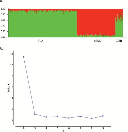
Results from STRUCTURE analyses (a) summary plot of individual Q values from Aetobatus narinari samples (b) identification of the number of populations (K) based on ΔK from STRUCTURE HARVESTER program using the method of Evanno et al. 2005.
First-generation migrants as detected by GENECLASS (GC) based on the Lhome statistic of Piry et al. (2004) along with corresponding STRUCTURE (STR) Q values
| Sample ID | Sex | Origin | GC Lhome | P-val | GC locality assigned | STR Q val |
|---|---|---|---|---|---|---|
| SER103 | F | FLA | 18.086 | 0.025 | Unsampled | 0.956 |
| SER148 | F | FLA | 19.750 | 0.031 | MXO | 0.809 |
| SER200 | F | FLA | 19.606 | 0.034 | Unsampled | 0.958 |
| SER213 | F | FLA | 20.206 | 0.024 | CUB | 0.955 |
| SER5050 | M | MXO | 15.115 | 0.012 | FLA | 0.903 |
| SER5059 | M | MXO | 19.034 | 0.031 | FLA | 0.842 |
| SERC007 | M | CUB | 20.462 | 0.034 | FLA | 0.740 |
| SERC010 | M | CUB | 20.184 | 0.042 | FLA | 0.616 |
| SERC011 | M | CUB | 20.360 | 0.035 | MXO | 0.626 |
| SERC014 | F | CUB | 20.636 | 0.032 | FLA | 0.526 |
Asymmetric migration rates from the program MIGRATE-N based on microsatellites. Results are given as the effective number of migrants per generation from each of the localities listed in rows on the left into those localities listed in columns on the right. The effective number of migrants per generation was calculated by multiplying M by θ of the receiving population and dividing by the inheritance scalar (4 for diploid organisms)
| FLA | MXO | CUB | |
|---|---|---|---|
| FLA | — | 95.0 | 258.6 |
| MXO | 70.3 | — | 128.3 |
| CUB | 27.2 | 15.2 | — |
| FLA | MXO | CUB | |
|---|---|---|---|
| FLA | — | 95.0 | 258.6 |
| MXO | 70.3 | — | 128.3 |
| CUB | 27.2 | 15.2 | — |
Discussion
In this study, we present the first data to support the existence of genetic heterogeneity among A. narinari populations in the Gulf of Mexico and northwestern Caribbean Sea region. As well, our study is the first to investigate fine-scale population structuring of this species using both nuclear and mitochondrial markers. Our results indicate that spotted eagle rays from the eastern and western parts of the Gulf of Mexico and the northern Caribbean Sea do not represent a single, panmictic population. However, while structure exists, weakly significant FST and ΦST values, coupled with shared haplotypes and seasonal abundance data (Cuevas-Zimbrón et al. 2011; Bassos-Hull et al. 2014), suggest a certain amount of genetic exchange is occurring. Gene flow between both Mexico and Cuba and Florida and Cuba localities appears high, with no significant differentiation detected by either the mtDNA or the nuclear DNA markers when sexes were both combined and analyzed separately.
An important consideration when interpreting results presented here is the fact that both spatial and temporal differences exist in the sampling strategy for each locality. First, although Florida samples were solely collected from shallow, coastal waters during dedicated survey efforts, samples from both Mexico and Cuba localities were collected opportunistically from either commercial fishing boats or local fish markets. As well, although surveys and sampling effort were conducted in Florida and Mexico across multiple seasons, all 19 samples from the southwestern Cuba locality were collected on 14 February 2013. Thus, results of comparisons with Cuba samples should be interpreted with caution as the sample size for this locality was much lower than the others and, unlike the other localities, samples were not distributed over time but rather all collected on a single day.
Genetic Diversity
Observed and expected heterozygosity estimates as well as allelic richness estimates were similar across the 3 sampling localities. Haplotype diversity was, on the other hand, higher for the Florida sampling locality though this may be an artifact of the higher sample size from this area. The overall range in diversity estimates based on both the microsatellites and mtDNA were comparable to estimates previously reported for both A. narinari and other batoid species (Sandoval-Castillo et al. 2004; Chevolot et al. 2006; Schluessel et al. 2010; Le Port and Lavery 2012). Average nucleotide diversity estimates (π) were low reflecting the low number of polymorphic sites present across sequences. These low values coincide with values reported for cytochrome b sequences of A. narinari in the Indo-Pacific (Schluessel et al. 2010). Results from our relatedness estimates did not suggest samples from any of the localities contained a high number of related individuals. However, samples from Cuba contained fewer related individuals than Florida or Mexico and this is likely an artifact of both the lower sample size and lack of temporal spread for samples collected at this locality.
Population Structure and Migration
Although Schluessel et al. 2010 reported high levels of population structure among A. narinari populations in the Indo-Pacific based on the mtDNA genes CytB and NADH4, subsequent work based on NADH2 (White et al. 2010; Naylor et al. 2012) and COI (Cerutti-Pereyra et al. 2012) suggest the Aetobatus species inhabiting the Indo-Pacific is not narinari but rather ocellatus and that, in fact, there may be another, distinct, undescribed species of Aetobatus off Vietnam. This latter scenario is further supported by a recent morphological study from White (2014). As such, it is likely that, as the authors suggest, the inclusion of more than 1 Aetobatus species contributed to the high levels of differentiation reported by Schluessel et al. (2010).
Although our genetic data reveal weakly significant population differentiation in the Gulf, ecological data suggest that movement of individuals, at least seasonally, is occurring. A field-based demographic study on A. narinari from our Sarasota Bay, Florida population documented consistent, seasonal fluctuations in observations of eagle rays over a 5-year period, with rays occurring in these coastal waters more frequently in late spring, summer, and autumn months and leaving the area in winter (Bassos-Hull et al. 2014). Seasonal fluctuations in abundance have also been reported in our Mexico population though, unlike Sarasota Bay, Florida, A. narinari abundance is highest off southeastern Mexico in winter months when sea temperatures are lowest (Cuevas-Zimbrón et al. 2011). This same seasonal trend of higher A. narinari abundance in winter months has been observed of rays off Cuba (Ruiz A, unpublished data) and Venezuela (Tagliafico et al. 2012). Off the island of Bimini, Bahamas, A. narinari are reported to be more abundant in the spring versus summer months (Silliman and Gruber 1999). Similar seasonal fluctuations in coastal ray abundance have been reported for other myliobatid and rhinopterid species such as Aetobatus flagellum (Yamaguchi et al. 2005), Myliobatis californica (Gray et al. 1997), and Rhinoptera bonasus (Blaylock 1993).
These studies, coupled with our genetic findings, support a seasonal migration of rays from the central west coast of Florida to northwestern Caribbean waters during winter months. Although more samples collected from Caribbean localities are needed to further strengthen this hypothesis, our STRUCTURE results do suggest the majority of samples collected off Cuba are from migrants originating from either Florida or Mexico. AMOVA analyses also indicate high gene flow between Mexico and Cuba localities as well as between Florida and Cuba. Historical estimates of migration support this with strong asymmetrical gene flow from both Gulf localities to the northern Caribbean Sea. Although the distance between either Mexico or Florida and our Cuban sampling area is shorter than that between Florida and Mexico, gene flow between either Mexico or Florida and the south side of Cuba suggests these rays may be migrating distances of at least 750 km. Satellite tagging data from 1 adult female A. narinari tagged off Sarasota Bay, Florida, showed southward movements during the summer of 2013, coming within approximately 55 km of the northwest coast of Cuba (Hueter R et al., unpublished data). This migration pattern is similar to what has been reported in the related batoid species R. bonasus (Schwartz 1990). Though Schwartz’s hypothesis was later challenged by Collins et al. 2007, other studies have supported long-distance migrations of Rhinoptera species (Grusha 2005) and Collins et al. (2007) proposed a seasonal migration route from the Yucatan peninsula to Florida for 1 R. bonasus population in the Gulf. In any case, the vagility of A. narinari, coupled with a lack of geographic barriers between these areas, suggest that such a migratory route and distance would be feasible for this species. Indeed the ability of A. narinari to swim great distances has been recognized by others (Compagno and Last 1999), though published accounts to support this do not currently exist. Long-distance migrations have also been reported in other batoid species such as L. ocellata (Frisk et al. 2010), and mobulid species in general are thought to undergo long-distance migrations (Couturier et al. 2012). Although limited tagging data have been reported for other elasmobranch species in this same study area, at least 1 study reports on the movement of tagged whale sharks between the Yucatan peninsula and both northern and southern sides of Cuba (Hueter et al. 2013).
Perhaps more surprising than the horizontal distance, this migration route suggests these rays are crossing through waters with depths greater than 1000 m. Little data exist documenting the depths at which many batoid species are found. At least 1 study reported the movements of some rajids to depths of about 1000 m (Stehmann and Bürkel 1994) and 1 Mobula japanica was tracked to 650 m depth (Francis 2014). In contrast, 2 months of satellite tagging data from the adult female A. narinari tagged off Sarasota Bay, Florida, showed that, although this ray did swim across deep waters (>800 m), its maximum dive depth was only 24.5 m (Hueter R et al., unpublished data). These data suggest that, although A. narinari can move across deep waters (i.e., deep waters do not appear to be a barrier to gene flow), they may only utilize depths in the upper photic zone.
Site Fidelity and Sex-Biased Dispersal
Recently, Feldheim et al. (2014) reported the first evidence of natal site philopatry in an elasmobranch species, N. brevirostris, sampled off Bimini, Bahamas. Site fidelity has also been suggested in certain batoid species such as Manta birostris (Dewar et al. 2008), but not in others, such as D. brevicaudata (Le Port and Lavery 2012). The recapture of approximately 6% of individuals in our Florida A. narinari population (including both males and females) over multiple years (Bassos-Hull et al. 2014) is consistent with our finding of genetic structure and suggests, though these rays move seasonally, they exhibit a certain amount of site fidelity to this area. Based on photo-identification data, Silliman and Gruber (1999) suggested seasonal residency in A. narinari found off Bimini. In R. bonasus, year-round residency has been suggested for at least 1 population in Pine Island Sound, Florida (Collins et al. 2007). Although our finding of genetic structure of A. narinari in the Gulf coincides with some level of site fidelity in this species, it appears the degree of site fidelity exhibited is not high enough to produce a strong genetic signal among our populations.
Given that male-biased dispersal has been reported in other elasmobranch species such as Isurus oxyrinchus (Schrey and Heist 2003), Carcharodon carcharias (Pardini et al. 2001), and Sphyrna lewini (Daly-Engel et al. 2012), we investigated our data for evidence of this trend in A. narinari. Although ΦST estimates for females alone for Florida versus Mexico were significant based on the mtDNA data (vs. nonsignificant for males), the opposite results were found between these populations when analyzing the microsatellite data, where males alone had significant FST values and females alone did not. (All comparisons with Cuba were nonsignificant regardless of sex and marker, but sample sizes per sex were small). This discordance in results between the 2 marker types is perplexing and underscores the importance of analyzing multiple marker types when making inferences about both population structure and sex-biased dispersal. Although mtDNA ΦST estimates were higher than those obtained from the microsatellite data, the magnitude of this difference was not high enough to rule out different marker characteristics (such as inheritance mode, ploidy, and mutation rate) being the cause. Results from GENECLASS did not indicate sex-biased dispersal as samples identified as first-generation migrants included equal numbers of both males and females. From these results, we are not inclined to suggest either sex of A. narinari is dispersing significantly more or less than the other, but that, taken together, genetic data presented here suggest both sexes are limiting their dispersal movements enough to maintain a low but significant amount of differentiation between the eastern and western parts of the Gulf. Further genetic investigation of sex-biased dispersal should include additional samples of known sex from our Cuba locality as well as separate analyses of juvenile versus adult samples. As our analyses included individuals from all age classes, it is possible the inclusion of juveniles in our sample reduced the strength of the nuclear markers to accurately detect sex-biased dispersal. Another option for further investigation of sex-biased dispersal in this system would be the application of kinship and parentage analyses. These methods have been used to identify philopatric behavior in some elasmobranch species (Feldheim et al. 2002, 2004; Portnoy 2008) and additional, extensive sampling of our Sarasota, Florida, population would deem them feasible for application to A. narinari.
Conservation Implications and Future Work
Given escalating threats to many elasmobranch species, the application of molecular markers to resolving aspects of their ecology, evolution, and conservation is imperative. Evidence presented here illustrating fine-scale genetic structure of A. narinari in the northeastern and southwestern parts of the Gulf of Mexico contributes valuable information towards current management plans for this species. Specifically, in areas where targeted A. narinari fisheries exist, a conservative approach should be taken when identifying management units. Given restricted gene flow across the Gulf, unsustainable fishing practices off both Mexico and Cuba could have significant effects on local populations. This is especially important in light of reports documenting the decline of this near-threatened species in fisheries over the last 5–10 years (Devadoss 1984; Kyne et al. 2006; Cuevas-Zimbrón et al. 2011).
Funding
California Academy of Sciences; Mote Scientific Foundation; Mote Marine Laboratory; Disney Worldwide Conservation Foundation; and the Save Our Seas Foundation.
Acknowledgments
We would like to thank Pete Hull, Dean Dougherty, Krystan Wilkinson, Ivan Méndéz-Loeza, Alexei Ruiz, Eloisa Rojas, and Roamsi Volta for their tremendous help in the field. We would also like to thank the local fishermen of both Mexico and Cuba for their assistance with sample collection. Previous versions of this manuscript were significantly improved from useful comments provided by 2 anonymous reviewers. All genetic data were generated in the Center for Comparative Genomics Lab at the California Academy of Sciences with assistance from Cerise Chen, Christopher Tanvilai, and Karmbir Chima.
References
Author notes
Data deposited at Dryad: http://dx.doi.org/doi: 10.5061/dryad.n914n
Corresponding editor: Jose Lopez
