


Summary
This study deals with the analysis of Swarm vector magnetic field measurements in order to estimate the magnetic field of magnetospheric ring current. For a single Swarm satellite, the magnetic measurements are processed by along-track spectral analysis on a track-by-track basis. The main and lithospheric magnetic fields are modelled by the CHAOS-6 field model and subtracted from the along-track Swarm magnetic data. The mid-latitude residual signal is then spectrally analysed and extrapolated to the polar regions. The resulting model of the magnetosphere (model MME) is compared to the existing Swarm Level 2 magnetospheric field model (MMA_SHA_2C). The differences of up to 10 nT are found on the nightsides Swarm data from 2014 April 8 to May 10, which are due to different processing schemes used to construct the two magnetospheric magnetic field models. The forward-simulated magnetospheric magnetic field generated by the external part of model MME then demonstrates the consistency of the separation of the Swarm along-track signal into the external and internal parts by the two-step along-track spectral analysis.
1 INTRODUCTION
The recovery of the 3-D electrical conductivity structure of the Earth’s mantle is one of the primary goals of the Swarm mission (Friis-Christensen et al. 2006). However, the results obtained so far within the framework of Swarm Level 2 processing suggest that it is also one of the most challenging tasks. The separation of the spatially and temporally variable magnetospheric magnetic field (MMF) from its induced counterpart has so far allowed only the 1-D mantle conductivity profile (Civet et al. 2015; Püthe et al. 2015; Grayver et al. 2017) to be recovered.
A possible reason as to why a more complex (and realistic) description of the mantle’s electrical conductivity has not yet been inferred is that the Swarm Level 2 model does not contain such information or suppresses it. The analysis of Swarm data for extracting the MMF faces a number of difficulties. Probably the most serious one is that the magnetic fields of PEJs and FACs dominate in the polar and near-polar regions, in particular, during geomagnetic storms, and overwhelm completely the X and Y components and significantly the Z component of the magnetic field generated by equatorial ring current in the magnetosphere (see Fig. 3 in this section). One way to overcome this problem is based on the comprehensive inversion (CI) scheme (Sabaka & Olsen 2006; Sabaka et al. 2013), which can be characterized by the following steps:
Three Swarm satellite and ground observatory data are analysed.
X, Y and Z residual magnetic signals (data) are analysed. These are obtained by subtracting the CI model from the original satellite and observatory data.
Only mid-latitude data are analysed.
Dayside and nightside data are analysed since the CI model contains the ionospheric component.
The magnetic potential, which describes X, Y and Z residuals, is represented as a sum of inducing and induced parts, and both are expanded into predefined sets of spherical harmonics. The inducing set contains the zonal and tesseral spherical harmonics of azimuthal order m = 1. The tesseral terms are introduced in order to describe the longitudinal dependence of magnetospheric source. The induced set contains more spherical harmonics than the inducing set to detect lateral variability of the Earth’s conductivity.
The spherical harmonic coefficients describing inducing and induced parts are estimated by an iterative reweighted least-squares method.
Throughout the paper, we will refer to the current version1 of the Swarm Level 2 magnetospheric field model obtained by the above approach as MMA_SHA|$\_2$|C.
Our aim in this paper is to extract the magnetic signals of magnetospheric ring current from the along-track satellite vector magnetic measurements made by a single Swarm satellite. We use the magnetic field vector, as given in the Level-1b products of the Swarm mission (Olsen et al. 2013). In addition to time and position, the data file contains the magnetic scalar intensity and the three components of the magnetic vector in the North-East-Center (NEC) local Cartesian coordinate frame.
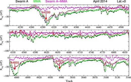
The Swarm A magnetic residuals ΔX (in nT) after subtracting the CHAOS-6 field model (black dots), the sum of the external and internal parts of the X component of model MMA_SHA|$\_2$|C (green dots) and the differences ΔXMMA between the two magnetic fields (violet dots) at the geographic equator on the nightsides from 2014 April 8 to May 10. The arrows with tracks numbers denote the tracks along which Swarm A measures the magnetic field at the main phases of two moderate storms and one minor storm. The respective 1 min USGS (thin red line) and 1 hr (thin blue line) Dst indices are shown for comparison.
Fig. 1 (also Fig. 2) shows that the residuals ΔXMMA reach 5 and 10 nT during magnetic quiet and magnetic storm times, respectively. Such large remaining residuals may be due to the ionospheric magnetic field, which may contribute to nightside track measurements. Fig. 2 therefore compares the residuals ΔXMMA with two current models of the magnetic field of the Earth’s ionosphere. The model MIO_SHA_2C2 (Sabaka et al. 2013) is estimated from Swarm and observatory data using the CI scheme within the Swarm Level 2 processing system. The model MIO_SHA_2D3 (Chulliat et al. 2016) is estimated by the dedicated ionospheric field inversion algorithm, which inverts a combination of Swarm satellite and ground observatory data at mid- to low latitudes and provides models of the solar-quiet and equatorial electrojet magnetic fields on the ground and at satellite altitude. Inspecting Fig. 2 we can see that the residual magnetic field ΔXMMA neither coincides nor correlates with either of the two ionospheric magnetic field models. On top of that, the two ionospheric magnetic field models significantly differ in amplitudes.
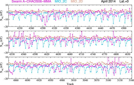
The Swarm A magnetic residuals ΔXMMA (in nT) after subtracting the CHAOS-6 field model and magnetospheric magnetic field model MMA_SHA|$\_2$|C (violet), and two models of the magnetic field of the Earth’s ionosphere, the model MIO_SHA_2C (light blue) and model MIO_SHA_2D (light brown), at the geographic equator on the nightsides for the Swarm A tracks considered in Fig. 1.
To test whether the results are independent of the choice of the geomagnetic main field and the lithospheric magnetic field, we have calculated an alternative set of residuals (1) by subtracting the current Swarm Level 2 main field model MCO_SHA_2C4and the lithospheric field model MLI_SHA_2C5from the Swarm measurements. Namely, these two models are used in the derivation of model MMA_SHA_2C within the Swarm Level 2 processing. The alternative geomagnetic main field and the lithospheric magnetic field have only negligible impact on the residuals (1). Hence, the residuals ΔXMMA shown in Figs 1 and 2 remains valid.
The fact that the remaining residual magnetic field ΔXMMA reaches unexpectably large amplitudes motivates us to develop an approach for estimating the MMF at satellite altitudes, which is independent of the CI based scheme (see Section 1) and provides an alternative way to estimate the magnetic signals of magnetospheric ring current from Swarm data.
The difficulty of any approach for estimating the MMF is demonstrated in Fig. 3, which shows the residuals ΔX and ΔZ along the Swarm B satellite tracks for two time intervals of 12 hr length. The residual magnetic field ΔZ changes with colatitude ϑ predominantly as the cosine of colatitude, that is, as the Legendre polynomial P10(cos ϑ), while the residual magnetic field ΔX changes as the sine of colatitude, that is, as the derivative of P10(cos ϑ) with respect to ϑ. This feature corresponds to the magnetic field generated by equatorial ring current in the magnetosphere. This regular feature is significantly disturbed by PEJs and FACs in the polar regions, and by mid- and low-latitude ionospheric electric currents on daysides. In fact, the Swarm data from polar regions must be omitted from the analysis for estimating MMF (see step 3 of the CI based scheme in Introduction). This creates a serious problem since about a third of along-tracks data are not considered in the analysis.
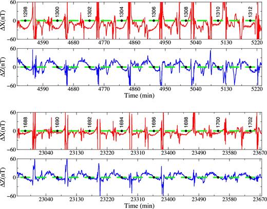
The magnetic residuals ΔX and ΔZ (in nT) after subtracting the CHAOS-6 field model along Swarm B satellite tracks for two time intervals of 12 hr length. Time (in min) is reckoned from 2014 January 1, 00:00:00 GMT. Green horizontal line segments indicate mid-latitudes between 60° south and 60° north. The full dots associated with the track numbers show the times when the satellite crosses the equator on the nightside.
One of our goals in this work is to compare the estimate of MMF by the method introduced in this paper with model MMA_SHA_2C. That is why we will limit the effect of daily ionospheric magnetic field variations by confining ourselves to Swarm data from along nightside satellite tracks for local times between 0:00 and 03:00. However, the method is applicable to Swarm data from along dayside satellite tracks if a model of the ionospheric magnetic field is implemented in the analysis.
As introduced, the disturbing effect of PEJs and FACs in the polar regions on estimating the MMF represents a serious problem. In this paper, similar to the CI based scheme we exclude the Swarm data from the polar regions and base the analysis for the MMF only on the Swarm data from mid-latitudes.
2 THE SPECTRAL REPRESENTATION OF THE RESIDUAL MAGNETIC FIELD AT SWARM SATELLITE ALTITUDES
3 THE TWO-STEP ALONG-TRACK SPECTRAL ANALYSIS OF SINGLE-SATELLITE MAGNETIC DATA
To analyse along-track satellite Swarm data, we adopt the method of Martinec & McCreadie (2004) with several modifications. For reasons of clarity, we will present the along-track spectral analysis in its completeness. Fig. 4 presents a workflow of the two-step spectral analysis of along-track Swarm data. The particular steps of the analysis are described in the following.
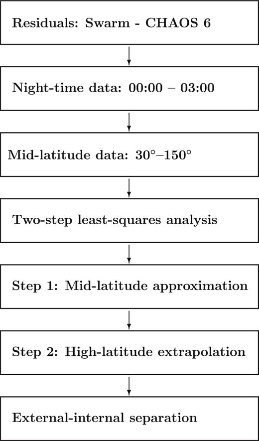
A workflow of along-track Swarm data processing.
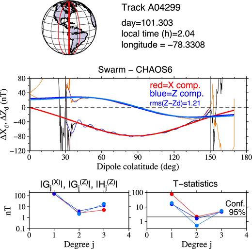
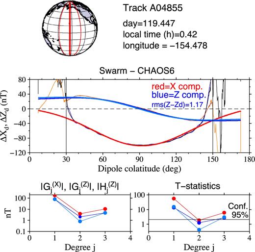
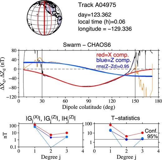
The two-step spectral analysis of the residual magnetic fields ΔXd and ΔZd along Swarm A satellite track A4299 for the estimation of the magnetospheric magnetic field. Top panel: Swarm A ground track under analysis (thick red), the previous and following ground tracks (thin red) with respect to the track under analysis. Second panel: the residual magnetic signals ΔXd (thin black) and ΔZd (thin orange) over the full-track nightside interval, the best-fitting signals (thin blue) after performing the first step of the spectral analysis over the dipole colatitudes (30°, 150°) and the best-fitting long-wavelength parts (j = 1 − 3) of ΔXd (thick red) and ΔZd (thick dark blue and thick light blue for the respective estimates described in Sections 3.2 and 3.3) by performing the second step of the spectral analysis. Left-hand bottom panel: The degree-amplitude spectra of coefficients |$G_{j,n}^{(X)}$| (red circles), |$G_{j,n}^{(Z)}$| (dark blue) and |$H_{j,n}^{(Z)}$| (light blue). Right-hand bottom panel: the T statistics of estimated coefficients |$G_{j,n}^{(X)}$|, |$G_{j,n}^{(Z)}$| and |$H_{j,n}^{(Z)}$|. The horizontal thin line denotes the critical value of the Student’s t-distribution at the 95 per cent significance level.
The analysis depends on a number of assumptions. The most important one concerns the geometry of the Swarm satellite tracks. Near-polar tracks of the Swarm satellites (the orbit inclinations are approximately 87.4° and 88.0° for Swarm A and B, respectively) supports the assumption of the analysis that the magnetic signal sampled along a track by the onboard magnetometer is influenced predominantly by the latitudinal variations of the Earth’s magnetic field. We thus implicitly assume that the longitudinal variations of the magnetic field cannot be revealed reliably from single-track Swarm measurements.
The input data of the spectral analysis are the samples of the residual magnetic fields ΔX and ΔZ along a satellite track, that is, two data sets (ri, ϑi, ΔXi) and (ri, ϑi, ΔZi), i = 1, …, D, where ri and ϑi are the geocentric radius and the colatitude of the satellite measurement side, respectively, and D is the number of data samples along the track. As commented upon earlier, the measured magnetic field in the polar regions is disturbed by PEJs and FACs. To minimize their effect, the polar regions are excluded from the analysis, leading to (ϑ1, ϑD) denoting the interval where the residual magnetic signals are analysed.
To set up eqs (6) and (7), the azimuthal order m of the spherical harmonics Yjm(Ω) and of spherical harmonic coefficients |$G_{jm}^{(X)}(r,t)$| and |$G_{jm}^{(Z)}(r,t)$| in eq.(4) is considered equal to zero, m = 0, and it is dropped from the notation. In addition, the zonal spherical harmonics Yj0(Ω) are equal to the fully normalized Legendre polynomials Pj(cos ϑ). Non-zero azimuthal orders cannot be considered in eqs (6) and (7) since the analysis is carried out for magnetic data along an individual single-satellite track. Hence, unlike the residuals ΔX and ΔZ, the presented along-track spectral analysis cannot be applied to the residual ΔY since the spherical harmonic representation (4) of the residual magnetic field ΔY is indefinite along latitude.
The CI algorithm discretizes the magnetosphere and associated magnetic induced fields in contiguous bins through time and considers them static within each bin (Sabaka et al. 2013). The degree-one spherical harmonic coefficients are sampled in 1.5 hr bins whereas other spherical harmonic coefficients in bins of 6 hr. We also parametrize the expansion coefficients |$G_j^{(X)}(t)$| and |$G_j^{(Z)}(t)$| by discretizing time into bins within which the coefficients are treated as static. All coefficients are sampled by the time tn when the Swarm satellite passes the equator, that is, they are sampled in approximately 1.5 hr bins. It also means that |$G_j^{(X)}(t_n)$| and |$G_j^{(Z)}(t_n)$| can be indexed by track number n, n = 1, 2, …, such that |$G_{j,n}^{(X)}\equiv G_j^{(X)}(t_n)$| and |$G_{j,n}^{(Z)}\equiv G_j^{(Z)}(t_n)$|. Moreover, we plot the 1 min USGS (Gannon & Love 2011) and 1 hr Dst indices for the period shown in Fig. 1. Comparing thin red and thin blue lines in Fig. 1 we can see that the two indices differ only very slightly, which supports the assumption on the magnetic field to be static within each time bin.
The along-track spectral analysis of residual magnetic signals ΔX and ΔZ is performed in two steps, a mid-latitude approximation and a polar-region extrapolation.
3.1 Mid-latitude approximation
In the first step, the mid-latitude data ΔXi and ΔZi are smooth in order to extrapolate them to polar regions (Section 3.2) and differentiate them with respect to co-latitude (Section 3.3). The smoothing, which is based on the approximation by a finite series of Legendre polynomials, can be derived as follows.
The coefficients |$A_j^{\prime }$| and |$B_j^{\prime }$| are estimated by the least-squares method applied separately to model equations (11) and (12). Hence, the least-squares estimates of |$A_j^{\prime }$| and |$B_j^{\prime }$| are independent of each other.
3.2 Polar-region extrapolation
In the second step, the two signals best fitting the mid-latitude data ΔXi and ΔZi are extrapolated from the mid-latitude interval (ϑ1, ϑD) to polar regions. The approach is as follows.
The cut-off degree jmax is a free parameter of the spectral analysis. In accordance with the parametrization of MMA_SHA_2C, it will be chosen as jmax = 3 in the following numerical examples. However, our numerical experiments with Swarm data showed that the choice of a larger cut-off degree jmax than 3 results in an unrealistic extrapolation of mid-latitude magnetic signals to the polar regions. For example, the extrapolated X component may have an extreme value in the polar regions, which does not correspond to the magnetic field generated by equatorial ring current in the magnetosphere.
3.3 An alternative: the along-track gradients of ΔZ
The application of the spectral analysis to a number of along-track Swarm residual magnetic signals ΔX and ΔZ showed that the extrapolation of long-wavelength parts of ΔX and ΔZ from mid-latitudes to polar regions suffers from a lack of data in the polar regions. This is particularly true for the signal ΔZ, since it is represented by Legendre polynomials Pj(cos ϑ) with the extreme values at the poles ϑ = 0 and ϑ = π. This causes the extrapolated signal ΔZ tends to have unrealistically large amplitudes in the polar regions. The extrapolation of ΔX is less affected by a gap in polar data, since it is represented by the derivatives of Legendre polynomials ∂Pj(cos ϑ)/∂ϑ with zero values at ϑ = 0 and ϑ = π. This means that the extrapolated signal ΔX tends to have small amplitudes in the polar regions, which is favourable behaviour when estimating the MMF, since its X component approaches zero at the poles.
Unrealistic behaviour of the extrapolated signal ΔZ in the polar regions therefore motivates us to design an alternative method for the extrapolation. The basic idea is to extrapolate the derivative of ΔZ with respect to ϑ, that is ∂ΔZ/∂ϑ, and not ΔZ itself. In such a case, termed the along-track gradient method, the derivative ∂Pj/∂ϑ spans ∂ΔZ/∂ϑ and the convergence of the extrapolated ∂ΔZ/∂ϑ to zero at ϑ = 0 and ϑ = π is guaranteed. The corresponding method can be derived as follows.
At this stage, three remarks need to be made. First, the along-track gradient method of the extrapolation of the long-wavelength part of the residual signal ΔZ from mid-latitudes to polar regions profits from the mid-latitude approximation described in Section 3.1. Without determining coefficients |$B_j^{\prime }$|, it would be problematic to differentiate raw satellite magnetic measurements. The smoothing of the residual signal ΔZ by fitting model (12) to raw satellite measurements is therefore an unavoidable step for the successful application of the along-track gradient method.
Second, if there are no polar gaps in the residual magnetic field, that is, when the mid-latitude interval (ϑ1, ϑD) is equal to (0, π), the respective methods based on ΔZ and ∂ΔZ/∂ϑ provide very similar estimates of the long-wavelength part of ΔZ, that is, |$G_{j,n}^{(Z)}\approx H_{j,n}^{(Z)}$|.
Third, Swarm A and Swarm C satellites currently fly on parallel tracks. Let us, however, imagine that they orbit one behind the other in the same orbital plane (which is, for instance, the case of the GRACE twin satellites). In this case, the long-wavelength part of ΔZ would be possible to estimate by three different approximations. Two approximations would be based on the extrapolation of ΔZ signals measured by the individual satellites. The third approximation would be based on the extrapolation of the derivative ∂ΔZ/∂ϑ determined by the differences of the ΔZ signals measured by the two satellites.
4 MAGNETOSPHERIC MAGNETIC FIELD ESTIMATION
As shown in Fig. 3, the largest contribution to the long-wavelength part of the residual magnetic fields ΔX and ΔZ originates in the magnetospheric large-scale ring current and the associated induced electric currents in the Earth. The respective currents generate the external (or primary) and internal (or secondary) magnetic fields. The sum of them, here called the MMF, will be estimated by the two-step spectral analysis of along-track magnetic data over the mid-latitude interval (30°, 150°). We have varied the endpoints of the interval by ±5° for the Swarm data along the tracks processed in Fig. 1, but the resulting estimate of the long-wavelength MMF does not seem sensitive to this. Since our analysis is carried out for a single-track data, we will estimate the magnetic field generated by equatorial ring current in the magnetosphere. We do not attempt to model the magnetic field of other magnetospheric sources, such as tail currents and magnetopause currents which may exhibit longitudinal asymmetries.
In accordance with the parametrization of the MMF by Sabaka & Olsen (2006), the spherical magnetic field components ΔX, ΔY and ΔZ in geographic coordinates are first transformed to ΔXd, ΔYd and ΔZd in dipole coordinates. The along-track spectral analysis of ΔXd and ΔZd is then carried out to estimate the dipole components Xd, MMF and Zd, MMF of the MMF. Finally, Xd, MMF and Zd, MMF are transformed back to the geographic components XMMF and ZMMF. For the backward transformation, the Y component of the MMF in the dipole coordinates is set equal to zero, Yd, MMF = 0. Note that this condition is satisfied only approximately for Swarm measurements, since the orbital plane of the Swarm satellites does not coincide exactly with the magnetic dipole meridional plane.
Figs 5–7 illustrate the results of the spectral analysis of the residual magnetic field along Swarm A satellite tracks A4299, A4855 and A4975. Swarm A along these tracks measures the magnetic field at the main phases of the magnetic storms shown in Fig. 1 (the arrows with track numbers). The satellite flew over the equator at longitudes 78.3308°, 154.478° and 129.336° west at local times 2.04, 0.42 and 0.06 hr on 2014 April 12, April 30 and May 4, respectively. The thick red line in the left-hand top panel shows the Swarm A ground track, while the two thin red lines show the previous and following tracks with respect to the track under analysis.
The second panel of Figs 5–7 shows the residual magnetic signals ΔXd (thin black line) and ΔZd (thin orange line) along the entire nightside track, while the filtered signals, after performing the first step of the spectral analysis over the mid-latitude interval (30°, 150°) are shown by thin blue lines. By choosing N΄ = 25, we can see that models (11) and (12) remove the high-frequency noise from the mid-latitude signals ΔXd and ΔZd and adjust both the long- and medium-wavelength parts of the data in a close way. The extrapolated long-wavelength parts of ΔXd and ΔZd from the mid-latitudes to the polar regions, by performing the second step of the spectral analysis (Section 3.2), are shown by the thick red and thick dark blue lines, respectively. The extrapolation of the long-wavelength part of ΔZd by the along-track gradient method (see Section 3.3) is shown by the thick light blue line. We can see that, except for the polar regions, the dark blue and light blue signals are very close to each other. The root mean squares of the differences between the dark blue and light blue magnetic signals over the mid-latitudes is shown in the right-hand top corner of the panel, and is equal to 1.56, 1.17 and 0.95 nT for the three tracks, respectively. Hence, the extrapolation of ΔZd is relatively insensitive to the applied extrapolation method. However, this is not always the case. The extrapolated ΔZd magnetic field by the two methods may significantly differ in the polar or near-polar regions. This is an indication that the Z component of the Swarm magnetic data is disturbed by the magnetic field arising from the complex electric current configuration in the polar or near-polar regions.
The degree-amplitude spectra of coefficients |$G_{j,n}^{(X)}$|, |$G_{j,n}^{(Z)}$| and |$H_{j,n}^{(Z)}$| are shown in the left-hand bottom panel of Figs 5–7. The spectra have a V-like shape, that is, the degree 1 and degree 3 spherical harmonic coefficients are greater than the degree 2 coefficient. As already found by Banks (1969), this feature corresponds to the magnetic field generated by equatorial ring current in the magnetosphere. The magnetic field perturbation associated with the ring current can be expanded in a series of odd-degree zonal spherical harmonics. He estimated that the term of degree j = 3 will contribute less than 10 per cent in an expansion of the ring current field over the surface of the Earth. We thus consider coefficients |$G_{j,n}^{(X)}$|, |$G_{j,n}^{(Z)}$| and |$H_{j,n}^{(Z)}$| as the estimate of magnetospheric magnetic signal.
5 TEST OF STATISTICAL SIGNIFICANCE
The results of the Student’s t-test applied to all coefficients |$G_{j,n}^{(X)}$|, |$G_{j,n}^{(Z)}$| and |$H_{j,n}^{(Z)}$| are shown in the right-hand bottom panel of Figs 5–7, where the horizontal thin line denotes the critical value of the Student’s t-distribution at the 95 per cent significance level. We can see that the coefficients |$G_{j,n}^{(X)}$|, |$G_{j,n}^{(Z)}$| and |$H_{j,n}^{(Z)}$| are statistically significant for j = 1 and j = 3 in all three cases. The coefficients |$G_{j,n}^{(X)}$|, |$G_{j,n}^{(Z)}$| and |$H_{j,n}^{(Z)}$| for degree j = 2 are not statistically significant, which means that the null hypothesis that the data do not depend on the second-degree Legendre polynomial is true. At the 95 per cent significance level the degree-two coefficients can be set equal to zero. This confirms Banks (1969) finding that the magnetic field of an equatorial ring current can be represented as a series of odd-degree Legendre polynomials only.
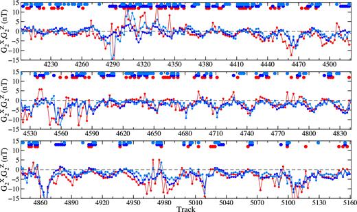
Fig. 8 shows the least squares estimates of coefficients |$G_{1,n}^{(X)}$|, |$G_{1,n}^{(Z)}$| and |$H_{1,n}^{(Z)}$| for the Swarm data along the tracks processed in Fig. 1. The red and blue dots at the top of the panels indicate that the associated coefficient is not statistically significant. We can make two conclusions. First, except for a very few cases, most coefficients |$G_{1,n}^{(X)}$|, |$G_{1,n}^{(Z)}$| and |$H_{1,n}^{(Z)}$| are statistically significant. Second, the differences between |$G_{1,n}^{(Z)}$| and |$H_{1,n}^{(Z)}$| are hardly recognizable, meaning that the extrapolation of ΔZd to polar regions is relatively insensitive to the applied extrapolation method.
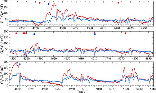
The least-squares estimates of coefficients |$G_{1,n}^{(X)}$| (red dots), |$G_{1,n}^{(Z)}$| (dark blue) and |$H_{1,n}^{(Z)}$| (light blue) for the tracks processed in Fig. 1. The red and blue dots at the top of the panels indicate that the associated coefficient is statistically insignificant.
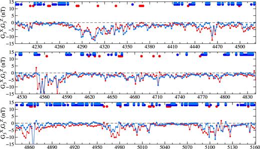
Similarly to Fig. 8, Figs 9 and 10 show the least squares estimates of coefficients |$G_{j,n}^{(X)}$|, |$G_{j,n}^{(Z)}$| and |$H_{j,n}^{(Z)}$| for degrees j = 2 and j = 3, respectively. We can see that there are as many insignificant coefficients as significant. It tells us that to use these time series for determining the electrical conductivity of the Earth’s mantle must be done with a certain reservation and the resulting conductivity model should be tested for its statistical significance. Moreover, the differences between |$G_{2,n}^{(Z)}$| and |$H_{2,n}^{(Z)}$| are now recognizable, which tell us that PEJs and FACs have a non-negligible effect on even-degree mid-latitude Swarm magnetic signals. On the contrary, the differences between |$G_{3,n}^{(Z)}$| and |$H_{3,n}^{(Z)}$| are less pronounced than for the degree 2 coefficients. Hence, odd-degree mid-latitude Swarm magnetic signals are less disturbed by the electric currents in the polar regions.
6 THE SEPARATION OF A SATELLITE SIGNAL INTO THE EXTERNAL AND INTERNAL PARTS
Having determined the coefficients |$G_{j,n}^{(X)}$|, |$G_{j,n}^{(Z)}$| and |$H_{j,n}^{(Z)}$| up to degree j = 3 along each satellite track, the external and internal Gauss coefficients, |$G_{j,n}^{(e)}$| and |$G_{j,n}^{(i)}$|, can be computed by inverting eq. (5) for each track. By this, the signal is separated into two parts having an external and an internal origin, respectively. From now on, we will refer to the MMF estimated by applying the two-step along-track spectral analysis and separated into the external and internal parts, as the MME model. It is important to emphasize that the separation is performed with respect to the Swarm satellite altitude. Hence, the magnetic field generated by magnetospheric ring current will be projected onto the external Gauss coefficients, while the magnetic field generated by the associated induced electric currents in the Earth will be projected onto the internal Gauss coefficients. On the contrary, the ionospheric electric currents and the associated induced currents in the Earth will generate two magnetic fields, both of which will be projected onto the internal Gauss coefficients only. Thus, there is no chance to separate the ionospheric magnetic field into the external and internal parts in Swarm data, but the ground observatory data must be taken into account to perform such a separation (Everett 2010; Olsen et al. 2010).
In the top panel of Fig. 11 we show the squared coherences between the external and internal coefficients of the MME model, calculated for degrees 1–3 from contiguous time series obtained for nightside tracks from July 1 to September 30, 2014. We note a high consistency between the inducing and induced signals at degree one and to a lesser extent also at degree two, while the internal degree-three coefficients appear not to be linearly related to the external field at the same spatial scale, except perhaps for periods around 120 hr.
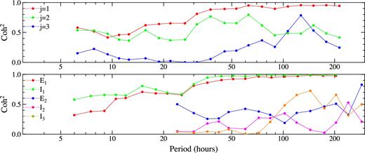
Top panel: Squared coherences between the external and internal field coefficients of the MME model for degrees one (red), two (green) and three (blue). Bottom panel: Squared coherences between the coefficients of MME and MMA_SHA_2C models. Red, green, blue, violet and orange dots correspond respectively to degree-one external, degree-one internal, degree-two external, degree-two internal, and degree-three internal harmonics.
In the bottom panel of Fig. 11, we use the squared coherences to compare the external and internal spherical harmonic coefficients provided by the MME and MMA_SHA_2C models. For this purpose, the same time series of the MME coefficients are spline-interpolated to a common sampling rate with the MMA_SHA_2C coefficients, that is, 1.5 hr for degree j = 1, and 6 hr for degrees j = 2 and 3. Since the recent MMA_SHA_2C model has the external field truncated at degree j = 2, only the internal coefficients are compared for degree 3. In the ideal case, the coherences between the MME and MMA_SHA_2C models should be close to one as both models attempt to describe the same magnetic fields. However, only the degree one coefficients, both external and internal, and perhaps the degree three internal coefficients in the period band of 100–200 hr, seem to be coherent.
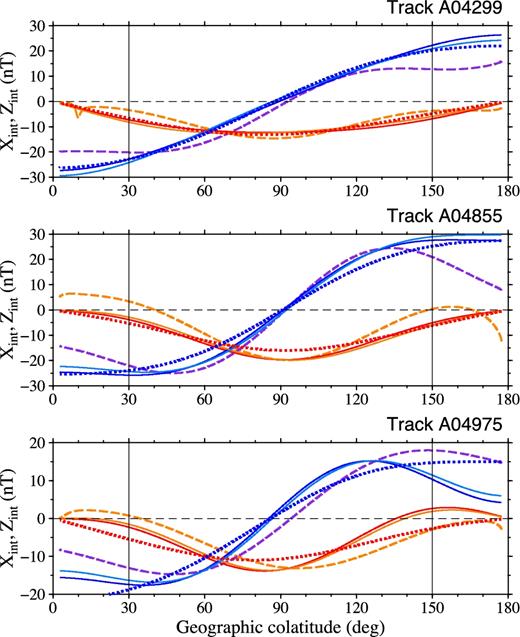
Fig. 12 shows the external parts of models MME and MMA_SHA_2C along the three tracks denoted in Fig. 1. We can see that the basic feature of the signals modelled by MME and MMA_SHA_2C are in a good agreement. However, there are also long-wavelength differences between the two signals, which may reach 10 nT as, for example, for the low-latitude X component along track A4975.
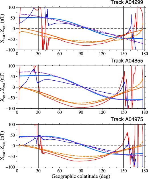
The external parts of models MME (solid red and blue lines for the X and Z components, respectively) and MMA_SHA_2C (dashed orange and violet lines for the respective components) along tracks A4299, A4855 and A4975. The magnetic residuals ΔX (thin red) and ΔZ (thin blue) are shown for comparison.
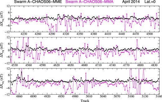
The Swarm A magnetic residuals ΔXMMA and ΔXMME (in nT) after subtracting the CHAOS-6 field model and magnetospheric magnetic field models MMA_SHA_2C (violet) and MME (black), respectively, at the geographic equator on the nightsides for the Swarm A tracks considered in Fig. 1.
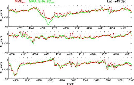
The external parts of the X component of models MME (red dots) and MMA_SHA_2C (green dots) at latitude 45° on the nightsides.
Figs 14 and 15 compare the external parts of the X and Z component of models MME and MMA_SHA_2C at latitude 45° on the nightsides. We can see that the MMA_SHA_2C and MME signals agree sufficiently well during geomagnetic quiet nights, but they may differ up to 10 nT during magnetic storm nights as, for example, the X component during the moderate magnetic storm for tracks from A4270 to A4350. A similar feature can be found at the southern hemisphere, for example, at latitude −45° (not shown here).
7 THE INTERNAL PART OF MAGNETOSPHERIC MODELS
Before discussing the internal parts of the MME and MMA_SHA_2C signals, it is useful to compare these two Swarm-based signals with the forward-simulated magnetic signals of magnetospheric origin. The simulations are done by the time-domain approach (Martinec et al. 2003) with electromagnetic forcing given by the external part of model MME. The electrical conductivity of the Earth’s mantle is considered to be spherically symmetric and is represented by the 1-D conductivity model by (Püthe et al. 2015). The model of MMF simulated from the external part of MME will be denoted as model MMS.
Fig. 16 shows the internal parts of the signals modelled by MME, MMA_SHA_2C and MMS, respectively, along the three tracks denoted in Fig. 1. We can make two conclusions. First, the internal signals of models MME and MMS agree sufficiently well. Note that we have not tuned the 1-D conductivity model to adjust the internal part of MME. The agreement means that the two-step spectral analysis decomposes the along-track Swarm signal in a consistent manner, such that the external and internal parts can be related by the physical process of electromagnetic induction in the Earth’s mantle.
Second, the basic feature of the signals modelled by MME and MMA_SHA_2C are in a good agreement. However, there are also long-wavelength differences between the two signals, which may reach 10 nT as, for example, in the Z component at high-latitudes. The differences probably arise from different treatment of Swarm data in near-polar regions. While the CI based scheme (see Section 1) estimates the inducing and induced signals by an iterative reweighted least-squares method, the two-step along-track spectral analysis extrapolates the X and Z signals from mid-latitudes to the polar regions and estimates the spherical harmonic coefficients of X and Z components by a non-iterative unweighted least-squares method.
Finally, Figs 17 and 18 compare the internal parts of the X and Z components of models MME, MMA_SHA_2C and MMS at the equator and latitude 45° on the nightsides, respectively. These figures confirm the conclusions made from Fig. 15. In addition, there is a possibility to tune the 1-D conductivity model by (Püthe et al. 2015), or introduce a 2-D mantle conductivity model, such that the internal part of model MMS will adjust the internal part of model MME even in a closer way than shown in Figs 16 and 17. For example, the X component of model MME during two moderate magnetic storms can still be adjusted more tightly.
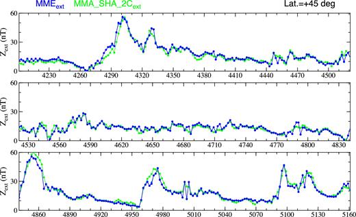
The same as Fig. 14, but for the Z component of models MME (blue dots) and MMA_SHA_2C (green dots).
The internal parts of models MME (solid red and blue lines for the X and Z components, respectively), MMA_SHA_2C (dashed orange and violet lines for the respective components) and MMS (dotted red and blue lines for the respective components) along tracks A4299, A4855 and A4875, respectively.
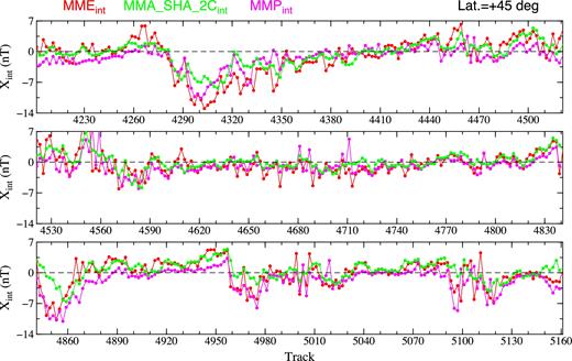
The internal parts of the X component of models MME (red dots), MMA_SHA_2C (green dots) and MMS (magenta dots) at the equator on the nightsides.
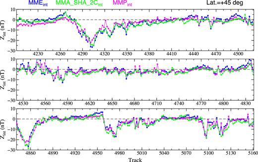
The internal parts of the Z component of models MME (blue dots), MMA_SHA_2C (green dots) and MMS (magenta dots) at latitude 45° on the nightsides.
8 CONCLUSIONS
The designed two-step spectral analysis method for estimating the signals of magnetospheric origin from along-track Swarm vector data can be summarized as follows (compare with the CI based method described in Section 1).
A single-satellite Swarm data are analysed.
X and Z residual magnetic signals (data) are analysed. These are obtained by subtracting the CHAOS model from the original satellite data.
Only mid-latitude data are analysed. The mid-latitude data are continued to polar-regions by an extrapolating scheme.
Only nightside data are analysed since the CHAOS model does not contain the ionospheric component. The method is applicable to dayside Swarm data if a model of the magnetic field of mid- and low-latitude ionospheric current systems is introduced.
The magnetic potential, which describes X and Z residuals, is represented as a superposition of three first zonal spherical harmonics. This means that longitudinal variations of the Earth’s conductivity and longitudinal dependence of the magnetospheric source are excluded from considerations.
The X and Z components are processed separately by the least-squares method of the continued signals along colatitude. The spherical harmonic coefficients of the inducing and induced parts of the signal are then obtained from the estimated X and Z spherical harmonic coefficients. The separate analysis of the X and Z components assumes the Swarm signals to be measured at the reference sphere with the radius equal to the mean radius of the Swarm satellite orbit.
The model of the magnetosphere (MME) obtained by the above scheme has been tested against two criteria. The first one, represented by the test T-statistic (23), determines whether the estimated spectral coefficients of the extracted signal are statistically significant in order to be considered for further processing. The second one, represented by the forward-simulated magnetic model, based on the external part of model MME, tests whether the external and internal parts of model MME are in agreement with the process of electromagnetic induction of the Earth. It is also complemented by the calculation of the squared coherences between the external and internal field coefficients. We have shown that the two-step along-track spectral analysis gives signal estimates that satisfy the two criteria. Although none of the criteria can uniquely confirm that the extracted signal is of a magnetospheric origin, two together provide good confidence that this is the case. Hence, we believe the method provides a reliable estimate of those signals of magnetospheric origin.
The model MME has been compared with model MMA_SHA_2C. Although the basic feature of the signals generated by MME and MMA_SHA_2C are in agreement, there are also differences reaching 5 nT and 10 nT during magnetic quiet and magnetic storm times, respectively. These differences are probably due to different processing schemes used to construct the two MMF models. In terms of spherical harmonic coefficients, the best agreement is obtained for degree one. Since any data processing method cannot provide a unique solution, the ’true’ MMF most probably lies between models MME and MMA_SHA_2C. This is therefore a task for future research in order to determine how to model PEJs and FACs when estimating the MMF.
A presented methodology of fitting a single Swarm satellite data by track-by-track basis functions allows estimating the magnetic field of the magnetospheric ring current. We have not attempted to model other magnetospheric sources, such as the magnetic field of tail currents and magnetopause currents. Nevertheless, by removing the magnetic fields of mid- and low-latitude ionospheric current systems, PEJs and FACs, all three Swarm satellite data can be processed simultaneously and longitudinal asymmetries of the MMF can be estimated. It is, however, challenging task for future research.
Acknowledgements
The authors would like to thank Kevin Fleming, Alexey Kuvshinov, an anonymous reviewer and G. Egbert, the handling editor of Geophys. J. Int., for their comments that have helped to improve the manuscript. This research was supported by the Grant Agency of the Czech Republic, project No. P210/17-03689S, the European Space Agency Contract No. 4000109562/14/NL/CBi ‘Swarm+Oceans’ under the STSE Programme and by the research programme 11/RFP.1/GEO/3309 financed by the Science Foundation of Ireland. The authors acknowledge these supports.
