Are geomagnetic data consistent with stably stratified flow at the core–mantle boundary?

Lesur, V.; Whaler, K.; Wardinski, I.

doi:10.1093/gji/ggv031

Abstract

Recent first principles calculations of the Earth's outer core thermal and electrical conductivities have raised their values by a factor of three. This has significant implications for geodynamo operation, in particular, forcing the development of a stably stratified layer at the core–mantle boundary (CMB). This study seeks to test the hypothesis of a stably stratified layer in the uppermost core by analysing geomagnetic observations made by the CHAMP satellite. An inversion method is utilized that jointly solves for the time-dependent main field and the core surface flow, where we assume the temporal variability of the main field, its secular variation (SV), to be entirely due to advective motion within the liquid outer core. The results show that a large-scale pure toroidal flow, consistent with a stably stratified layer atop the outer core, is not compatible with the observed magnetic field during the CHAMP era. However, allowing just a small amount of poloidal flow leads to a model fitting the observations satisfactorily. As this poloidal flow component is large scale, within a predominantly toroidal, essentially tangentially geostrophic flow, it is compatible with a stably stratified upper outer core. Further, our assumption of little or no diffusive SV may not hold, and a small amount of SV generated locally by diffusion might lead to a large-scale pure toroidal flow providing an acceptable fit to the data.

Magnetic field, Rapid time variations, Satellite magnetics

1 INTRODUCTION

Magnetic data are one of the rare sources of information about the motion of the iron-rich liquid forming the outer core of the Earth. It is generally accepted that the Earth's magnetic field is generated mainly in the outer core by convective flows associated with heat and light element release due to the slow freezing of the Earth's inner core. A better understanding of the evolution of the Earth's deep interior is therefore closely linked to our ability to describe this outer core flow. The magnetic field and core flow are related through the induction equation, derived directly from Maxwell's equations.

Most approaches begin by deriving magnetic field models from measurements at the Earth's surface and satellite altitude. These models are then used to deduce the flow in the core, even if the modelling step somehow filters out part of the information available in the data. Several difficulties limit further our ability to describe the core flow.

First, the magnetic field is measured at the Earth's surface and, after neglecting mantle electrical conductivity to allow the field to be downward continued to the core–mantle boundary (CMB), only the radial component of the poloidal part of the magnetic field is continuous across the conductivity jump there. This component can reasonably be estimated at the top of the free stream, just under the liquid viscous boundary layer (Roberts & Scott 1965; Jault & Le Mouël 1991). However, it is available only for the longest wavelengths, because the field generated in the lithosphere hides core field wavelengths shorter than about three thousand kilometres. The toroidal magnetic field, the small-scale radial poloidal field and the horizontal poloidal field components, all present inside the core, are not accessible from magnetic data without further assumptions.

A second difficulty is that, assuming we are able to describe the large-scale (poloidal) radial magnetic field and its slow rate of change, the secular variation (SV), at the top of the core, it is still not possible to derive the fluid flow in the core uniquely, not even the flow on the spherical surface approximately defined by the top of the free stream. One aspect of the problem is the presence of magnetic diffusion in the core. Following Roberts & Scott (1965), numerous authors interested in flow estimation simply neglect it, although this approach has been questioned (Gubbins 1996; Love 1999). It is however generally accepted that it is a reasonable first order approximation on relatively short time and long length scale field components (see e.g. Jackson & Finlay 2007, for a review). When magnetic diffusion is neglected, the field is frozen in to the liquid and moves with it; thus, neglecting diffusion is often called the frozen-flux assumption (see e.g. Backus et al.1996). A further issue is that the unknown small-scales of the magnetic field can interact with the small scales of the flow to generate large-scale SV (Hulot et al.1992). Therefore, only part of the information carried by the observed SV can be used to explain the large scale flow. A final important aspect is that we have just one equation, the induction equation, defining two unknowns: the horizontal components of the flow (we assume the top of the free stream represents a material boundary, so its radial component vanishes). The resulting non-uniqueness was well characterized by Backus (1968). Only very strong hypotheses on the flow geometry and correlation length scale can reduce or resolve the non-uniqueness. One such hypothesis is the absence of poloidal flow at the top of the free stream, which is compatible with strong stratification of the top-most part of the outer core (Whaler 1980). In the last few years, the suggestion that the top of the core is stably stratified has been strongly supported by studies including those of Helffrich & Kaneshima (2010), Pozzo et al. (2012) and Gubbins & Davies (2013). Helffrich & Kaneshima (2010) find that the top of the core must be compositionally stratified, enriched by up to 5 weight per cent in light elements, to fit the observed seismic wave speed data. Pozzo et al. (2012) estimate the thermal and electrical conductivity of the core using first-principle techniques, resulting in an increase in core conductivity by a factor three over previous estimates, under which scenario the core evolves to have a stratified layer adjacent to the CMB. Gubbins & Davies (2013) suggest that the stratification results from the barodiffusion of light elements, forming a layer at the top of the core that would resists the effect of convection. In this case, the stratification is likely to be very strong.

Assuming the flow is essentially large scale, the purely toroidal flow hypothesis can be tested against the measured SV at the Earth surface. This has been undertaken several times in the past (Whaler 1980, 1984, 1986; Bloxham 1990) but the results have not been sufficiently conclusive to definitively support, or reject, the hypothesis. One of the major difficulties to overcome is the quality of the magnetic field model used. In particular it is difficult to assess how the constraints applied during the field model estimation process affect the test. In this paper, we want to look again at this issue, firstly because high quality low Earth orbiting CHAMP satellite data allow for a more precise description of the core field, and secondly, because we can use Field-Flow co-estimation techniques (Lesur et al.2010a) that allow the hypothesis to be tested by direct comparison with magnetic data rather than relying on field models which are sequentially inverted for the core surface flow. To provide robust results the method should control carefully the error budgets of both the induction equation and the magnetic field data collected, in this case, by CHAMP.

The paper is organized as follows: in the next section, we describe the magnetic field and flow model parametrizations. In the third section we present CHAMP data selection and inversion schemes. We also describe the handling of the errors, including those in the radial component of the induction equations. The results are given in the fourth and discussed in the fifth sections.

2 MODEL PARAMETRIZATION

Away from its sources, the magnetic field can be described as the negative gradient of potentials associated with sources of internal and external origin:

\begin{eqnarray} && \mathbf {B}= \mathbf {-\nabla } \lbrace V_i\left(\theta ,\phi ,r,t\right) + V_e(\theta ,\phi ,r,t) \rbrace \nonumber\\ && V_i(\theta ,\phi ,r,t)= a \sum _{l=1}^{L_i}\sum _{m=-l}^{l} \left(\frac{a}{r}\right)^{l+1} g_l^m(t) Y_l^m(\theta , \phi )\nonumber\\ && V_e(\theta ,\phi ,r,t)= a \sum _{l=1}^{L_e}\sum _{m=-l}^{l} \left(\frac{r}{a}\right)^{l} q_l^m(t) Y_l^m(\theta , \phi ), \end{eqnarray}

(1)

where |$Y_{l}^{m}(\theta ,\phi )$| are the Schmidt semi-normalized spherical harmonics (SHs). θ, ϕ, r, a are the colatitude, longitude, satellite altitude and model reference radius, respectively, in geocentric coordinates. We use the convention that negative orders, m < 0, are associated with sin (|m|ϕ) terms whereas null or positive orders, m ≥ 0, are associated with cos (mϕ) terms.

At satellite altitudes, the surrounding medium is a conductive plasma, but we do not parametrize toroidal fields generated there. The internal part of the magnetic field is associated with three different sources, namely the core, the lithosphere and the magnetic field induced in the conductive layers of the Earth by all fields varying rapidly in time relative to an Earth-fixed system of coordinates. For the largest wavelengths of the field generated in the core and lithosphere (here, assumed up to SH degree L_i = 18), the reference radius used in equation (1) is a = 3485 km. The Gauss coefficients are parametrized in time from 2000.0 to 2011.5, using order six B-splines |$\psi ^6_{i}(t)$|⁠, with half-year time interval between spline nodes. The time dependence of the Gauss coefficients is therefore given by:

\begin{equation} g_{l}^{m}(t)=\sum _{j=1}^{N_{t}}g_{lj}^{m} \, \psi ^6_{j}(t), \end{equation}

(2)

where N_t = 28.

For the core and lithospheric field of SH degree greater than 18, the reference radius in eq. (1) is set to a = 6371.2 km. They are assumed to be constant in time, which is probably unrealistic for the core field, but these contributions cannot practically be distinguished from observational noise and are therefore unresolved. The lithospheric field also varies in time, but on time scales that are so much longer than the time span of our data set that we can neglect them (Hulot et al.2009). The maximum SH degree used for modelling the field of internal origin is 30, although a constant field covering all SH degrees from 20 to 60 (taken from Lesur et al.2013) is subtracted from the data so that only very small contributions from the lithospheric field remain unmodelled. Therefore the estimated Gauss coefficients from SH degrees 20 to 30 are effectively only a correction to those of the subtracted model.

The remaining parts of the internal field are the induced fields that are modelled using only one coefficient scaling the internal part of the Dst index, denoted Ist (Maus & Weidelt 2004; Olsen et al.2005), for 100-d time intervals. We use 36 of these 100-d intervals to account for possible base-line errors in Ist over the time span of the data set. The length of the time intervals was chosen to be long enough to avoid an overparametrization of the field, but different from an integer portion of a year or of the local time periodicity of the CHAMP satellite. Of course, this may lead to a discontinuous representation of the induced fields. The time dependence of the Gauss coefficient |$g_1^0(t)$| in eq. (2) is therefore modified to:

\begin{equation} g_{1}^{0}(t)=\sum _{j=1}^{N_{t}}g_{1j}^{0} \, \psi ^6_{j}(t) + \sum _{j=1}^{N_{i}}\tilde{g}_{1j}^{0} \, {\cal H}_j({Ist})\,, \end{equation}

(3)

where the function |${\cal H}_j(X)$| takes the value X in the time interval [t_j: t_j+1] and is zero otherwise. We have N_i = 36 spanning 2001.0–2010.75.

The external field parametrization also consists of independent parts. A contribution to the external field is modelled up to SH degree 20 without any time dependence in an Earth fixed system of coordinates. There is no justification for this part of the model other than the observation that it reduces some artefacts present in the residuals. On the other hand, by being constant in time this SH degree 20 external field has limited correlation with the rest of the model. A slowly varying part of the external field model is parametrized by a single degree l = 1 order m = 0 coefficient in the geocentric solar magnetic (GSM) system of coordinates. Further, over every 100-d time interval, two coefficients of SH degree l = 1, with orders m = 0 and m = −1, are estimated in a solar magnetic (SM) system of coordinates. This combination of GSM and SM parametrization is a simplified version of the parametrization proposed by Maus & Lühr (2005), but it models efficiently a significant part of the external fields. The rapidly varying part of the external field is controlled using the SVMD index (Kunagu et al.2013). Here again 100-d time intervals are used. Four scaling coefficients for the SVMD are introduced in each interval. Three are used for SH degree l = 1 and orders m = −1, 0, 1 and one for SH degree l = 2 and order m = 0. The scaling coefficient at SH degree l = 2 proves to be necessary to avoid latitudinal dependence of the data residuals. Overall the parametrization of the external field is:

\begin{eqnarray} &&{\mathbf {B}_e(\theta ,\phi ,r,t)=- \nabla \left[ a \sum _{l,m}^{L_e=20} \left(\frac{r}{a}\right)^{l} q_l^m \,Y_l^m(\theta , \phi ) \right]} \nonumber\\ &&{\quad-\, {\cal R}_{GSM} \nabla \left[ r \; q_1^{0 {\rm GSM}} \, Y_1^0(\theta , \phi ) \right] }\nonumber\\ &&{\quad-\, {\cal R}_{SM} \; \nabla \left[ r \sum _{j=1}^{N_{i}} \big\lbrace \,q_{1j}^{0 {\rm SM}} \, Y_1^0(\theta , \phi ) + \; q_{1j}^{-1 {\rm SM}} \, Y_1^{-1}(\theta , \phi ) \big\rbrace \; {\cal H}_j(1) \right]} \nonumber\\ &&{\quad -\, \sum _{j=1}^{N_{i}} \nabla \Bigg[ r \Bigg\lbrace \sum _{m=-1}^{1} (q_{1j}^{m {\rm SVMD}} \, Y_1^m(\theta , \phi ) {\cal H}_j({\rm SVMD}_m) }\nonumber\\ &&{\qquad\qquad +\, \left(\frac{r}{a}\right) q_{2j}^{0 {\rm SVMD}} \, Y_2^0(\theta , \phi ) {\cal H}_j({\rm SVMD}_0) \Bigg\rbrace \Bigg],} \end{eqnarray}

(4)

where |${\cal R}_{{\rm GSM}}$| and |${\cal R}_{{\rm SM}}$| are rotation matrices giving in Earth fixed geographic reference frame vectors defined in GSM and SM reference frames, respectively. The SVMD_m, m = −1, 0, 1 stands for the SVMD components along the Earth's rotation axis (Z-axis, m = 0), the direction perpendicular pointing to Greenwich meridian (X-axis, m = 1) and the last direction forming a right-hand oriented orthogonal system of coordinates (Y-axis, m = −1). The total number of parameters for the magnetic field is therefore 11 373, where 10 080 are used exclusively for the parametrization of the time varying core field.

In the framework of the field-flow co-estimation technique we need also to define a model for the flow. We follow here the classic approach that parametrizes the flow through its poloidal and toroidal scalars (e.g. Holme 2007). These are parametrized up to SH degree L_F = 20 with the same temporal dependency as the core field, that is B-splines of order six, with the spline nodes half a year apart and at the same positions as the nodes defined for the core field. Hence the flow at the top of the free stream, U_h, can be expressed as

\begin{eqnarray} {\mathbf {U}}_h(t,\theta ,\phi ,r) = \nabla _{h}\times (\hat{\mathbf {r}}{T})+ \nabla _{h}({S}), \end{eqnarray}

(5)

\begin{eqnarray} \mbox{ where } \left\lbrace \begin{array}{l}T=\sum _{l=1}^{L_{F}}\sum _{m} t_{l}^{m}(t)Y_{l}^{m}(\theta ,\phi ) \\ S=\sum _{l=1}^{L_{F}}\sum _{m} s_{l}^{m}(t)Y_{l}^{m}(\theta ,\phi ) \end{array} \right. \end{eqnarray}

(6)

\begin{eqnarray} \mbox{ and } \left\lbrace \begin{array}{l}t_{l}^{m}(t)=\sum _{i=1}^{N_{t}}t_{li}^{m}\psi ^6 _{i}(t) \\ s_{l}^{m}(t)=\sum _{i=1}^{N_{t}}s_{li}^{m}\psi ^6 _{i}(t) . \end{array} \right. \end{eqnarray}

(7)

∇_h denotes the horizontal part of the del operator on the unit sphere.

Under the frozen-flux assumption, the flow is related to the magnetic field and its SV through the radial component of the diffusion-less induction equation:

\begin{equation} \partial _{t}B_{r}=- \frac{1}{c} \nabla _{h}\cdot ({\mathbf {U}}_hB_{r}), \end{equation}

(8)

where c is the core radius. In the present application we use, as in Baerenzung et al. (2014), only a filtered version of this equation such that the influence of the unknown small scales of the magnetic field and the flow can safely be neglected. The full derivation of the filtered induction equation in the SH domain is given in Appendix A. The induction equation in its filtered form is:

\begin{equation} \partial _t \tilde{B}_r(\theta ,\phi ,t) = - \frac{1}{c} \nabla _h \cdot {(\tilde{\mathbf {U}}_h \tilde{B}_r)} - \frac{1}{c} \nabla _h \cdot {\tau }, \end{equation}

(9)

where the |$\tilde{.}$| indicates filtered (or smoothed) quantities, and τ is the difference between a filtered product and the product of the filtered quantities. It can be shown (Baerenzung et al.2014, see also Appendix A) that:

\begin{equation} {\tau} = 2 \; \lambda \; ( \nabla _h \tilde{B}_r \cdot \nabla _h ) \tilde{\mathbf {U}}_h, \end{equation}

(10)

where λ is dependent on the size of the smoothing filter. We used a filter size of 500 km as proposed by Baerenzung et al. (2014), which corresponds to λ = 8.5 × 10⁻⁴ in eqs (10) and (A10).

When a pure toroidal flow is modelled, the poloidal scalar coefficients |$s_l^m(t)$| are all set to zero, and the number of parameters reduces from 2 N_t × L_F(L_F + 2) for a general flow to N_t × L_F(L_F + 2) for a purely toroidal flow. With L_F specified as 20, these correspond to 24 640 and 12 320 parameters, respectively.

3 DATA SELECTION AND INVERSION SCHEME

The study is based entirely on data collected by the CHAMP satellite, which was launched in 2000 and flew until the second half of 2010. We used the data set version 2.6.51, which is remarkably homogeneous. Nonetheless, before mid-June 2001 the data are not fully processed and therefore do not have the same quality as during later periods. Similarly, due to the instruments and satellite ageing, the data quality at the end of the mission is slightly degraded. Despite this, we used the full data set, and selected the data in a very similar way as for the GRIMM-2 model (Lesur et al.2010b). These criteria are repeated below for completeness:

The vector data are considered in the SM coordinate system between ±55° magnetic latitude for magnetically quiet times according to

Positive value of the z-component of the interplanetary magnetic field (IMF-B_z) to minimize possible reconnection of the magnetic field lines with the interplanetary magnetic field (IMF);
Sampling points are separated by 20 s at minimum, such that the non-modelled lithospheric field does not generate correlated errors between data points;
Data are selected at local time between 23:00 and 05:00, with the sun below the horizon at 100 km above the Earth's reference radius (a = 6371.2 km), to minimize the contribution from the magnetic field generated in the ionosphere;
Norm of the vector magnetic disturbances (VMD, Thomson & Lesur 2007) should be less than 20 nT and norm of its time derivative less than 100 nT d⁻¹;
High accuracy of the fluxgate magnetometer (FGM) readings (quality flag 1 set to 0) and dual star-camera mode (quality flag 2 set to 3);
Star camera outputs checked and corrected (Flag digit describing the attitude processing technique larger than 1).

At high latitudes, that is polewards of ±55^o magnetic latitude, the three component vector magnetic satellite data are used in North, East Centre (NEC) system of coordinates. Their selection criteria differ from those listed above in two ways:

Data are selected at all local time, and independently of the sun position.
Data sampled in single-camera mode are used when no other vector data are available.

It was shown by Lesur et al. (2008) that using vector data in place of total intensity data at high latitudes allows for a better separation of the internal magnetic field from the ionospheric magnetic field when satellite data are selected at all local times. Altogether, these selection criteria lead to a relatively large data set consisting of N_d = 6 686 496 field values.

The linear relationship between data and magnetic field model parameters is given in eqs (1)–(4). This leads to a system of equations

\begin{equation} {\mathbf {d}}= {\mathbf {A}}_{d} \cdot {\mathbf {g}}, \end{equation}

(11)

where the vector d contains the full set of magnetic data values, and g contains all the magnetic field model parameters. As in the GRIMM series of field models, the data along the Z_SM direction are not used to estimate the internal field parameters. The set of eqs (11) does not allow unique resolution of the vector g, and further constraints have to be applied to solve for the Gauss coefficients. With the chosen field parametrization, this is necessary only for the internal Gauss coefficients. We therefore impose the constraint that the field varies smoothly in time by minimizing the integral over the model time span of the third time derivative squared of the core magnetic field radial component. We also require the radial component of the secular acceleration (SA) to be small at the model end points. This approach is presented in detail by Lesur et al. (2010b) and leads to a linear system of equations:

\begin{equation} {\mathbf {0}}= {\mathbf {L}}_{B} \cdot {\mathbf {g}}, \end{equation}

(12)

that are scaled by a multiplier λ_B to be solved together with eqs (11).

Quantities in the radial component of the frozen-flux induction eq. (9) are expanded in SH, and manipulated as described in Appendix A to give eqs (A25) and (A33) relating the magnetic field Gauss coefficients and the flow parameters. We proceed in the same way as Lesur et al. (2010a) and write the parametrized form of eq. (9), only up to SH degree 13, as a linear system that depends either on the Gauss coefficients or on the flow coefficients:

\begin{equation} \begin{array}{ll}\dot{\mathbf {g}}= {\mathbf {A}}_{B} \cdot {\mathbf {u}} \\ \dot{\mathbf {g}}= {\mathbf {A}}_{U} \cdot {\mathbf {g},} \end{array} \end{equation}

(13)

where u are the flow coefficients defined by eqs (5)–(7) and the vector |$\dot{\mathbf {g}}$| is calculated using a differential operator applied to g:

\begin{equation} \dot{\mathbf {g}} = {\mathbf {D}} \cdot {\mathbf {g}}\,. \end{equation}

(14)

The set of eqs (13) are time dependent and are established and weighted following a Gaussian integration rule (Abramowitz & Stegun 1964), such that a polynomial of degree 3 is integrated exactly between spline nodes.

It is well known (see e.g. Holme 2007) that there is an infinite number of solutions for u, and therefore further constraints have to be applied to the flow. We require the flow to be essentially large scale by minimizing the Bloxham ‘strong norm’ (Bloxham 1988b; Jackson 1997). Setting this constraint on the flow limits the possible SV evolution through eqs (13) and therefore smoothes the temporal field variations. This in turn leads to smooth flow temporal evolution. As a result it is not necessary to impose further temporal smoothing on the flow. Minimizing the Bloxham strong norm leads to a system of linear equations:

\begin{equation} {\mathbf {0}}= {\mathbf {L}}_{U} \cdot {\mathbf {u}}, \end{equation}

(15)

that are scaled by a multiplier λ_U to be solved together with eqs (13). The reader is referred to Lesur et al. (2010a) for details of setting up eqs (11)–(15).

We find the regularized least-squares solution by minimizing the functional:

\begin{eqnarray} &&{\Phi = \left[ {\mathbf {d}}-{\mathbf {A}}_{d} \cdot {\mathbf {g}} \right]^t {\mathbf {W}}_d \left[ {\mathbf {d}}-{\mathbf {A}}_{d} \cdot {\mathbf {g}} \right] + \lambda _B \left[{\mathbf {L}}_{B} \cdot {\mathbf {g}}\right]^t \left[{\mathbf {L}}_{B} \cdot {\mathbf {g}}\right]} \nonumber\\ &&{\,+\, \tilde{\lambda }\left\lbrace \left[ \left( {\mathbf {A}}_{U} - {\mathbf {D}}\right) \cdot {\mathbf {g}} \right]^t {\mathbf {C}}_{\dot{\mathbf {g}}}^{-1} \left[ \left( {\mathbf {A}}_{U} - {\mathbf {D}}\right) \cdot {\mathbf {g}} \right] + \lambda _U \left[{\mathbf {L}}_{U} \cdot {\mathbf {u}}\right]^t \left[{\mathbf {L}}_{U} \cdot {\mathbf {u}}\right] \right\rbrace , }\nonumber\\ \end{eqnarray}

(16)

for the vectors of parameters g and u. The scaling factor |$\tilde{\lambda }$| is introduced so that eqs (13) and (15) are fit to their expected level. The weight λ_U is modified to |$\lambda _U^T$| and |$\lambda _U^P$| if different scaling factors are required for toroidal and poloidal flows. Since the field and flow parameters enter as products in (13), the problem is non-linear and is solved through an iterative process. At iteration i the system of equations is:

\begin{eqnarray} \mathbf {W}_d^{\frac{1}{2}} \; \left[ {\mathbf {d}}-{\mathbf {A}}_{d} \cdot {\mathbf {g}}_i \right] &=& {\mathbf {W}}_d^{\frac{1}{2}} \; \left[ {\mathbf {A}}_{d} \cdot \delta {\mathbf {g}} \right] \nonumber\\ \tilde{\lambda }^{\frac{1}{2}} {\mathbf {C}}_{\dot{\mathbf {g}}}^{-\frac{1}{2}} \; \left[ -\left( {\mathbf {A}}_{U_i} - {\mathbf {D}}\right) \cdot {\mathbf {g}}_{i} \right] &=& \tilde{\lambda }^{\frac{1}{2}} {\mathbf {C}}_{\dot{\mathbf {g}}}^{-\frac{1}{2}} \! \left[ \left( {\mathbf {A}}_{U_i} \!- {\mathbf {D}}\right) \cdot \delta {\mathbf {g}} + {\mathbf {A}}_{B_i} \cdot \delta {\mathbf {u}} \right] \nonumber\\ \lambda _B^{\frac{1}{2}} \; \left[ - {\mathbf {L}}_{B} \cdot {\mathbf {g}}_{i} \right] &=& \lambda _B^{\frac{1}{2}} \; \left[ {\mathbf {L}}_{B}\cdot \delta {\mathbf {g}} \right] \nonumber\\ \tilde{\lambda }^{\frac{1}{2}} \lambda _U^{\frac{1}{2}} \; \left[ - {\mathbf {L}}_{U} \cdot {\mathbf {u}}_{i} \right] &=& \tilde{\lambda }^{\frac{1}{2}} \lambda _U^{\frac{1}{2}} \; \left[ {\mathbf {L}}_{U}\cdot \delta {\mathbf {u}} \right] \end{eqnarray}

(17)

with:

\begin{equation} \begin{array}{l}\mathbf {g}_{i\!+\! 1}={\mathbf {g}}_{i} + \delta {\mathbf {g}}\\ {\mathbf {u}}_{i\!+\! 1}={\mathbf {u}}_{i} + \delta {\mathbf {u}}. \end{array} \end{equation}

(18)

We postpone to towards the end of this section the definition of the starting models and proceed with a description of the equation weights.

The weight matrix W_d in eq. (16) should be the inverse of the data covariance matrix. We assume this is a diagonal matrix, and the data prior standard deviations are listed by data type in Table 1. However, the data errors do not follow a Gaussian distribution so an iterative reweighted least-squares (IRLS) method is used (Farquharson & Oldenburgh 1998), where the new weights are similar to Huber weights. For a datum d_j at iteration i, the associated weight is:

\begin{equation} {w}_{dj} = \left\lbrace \begin{array}{ll}\frac{1}{\sigma _j^2} &\mbox{ for } |{d}_j-{\mathbf {A}}_{dj} \cdot {\mathbf {g}}_i| \le k_j, \\ \frac{1}{\sigma _j^2} \left[ \frac{k_j}{|{d}_j-{\mathbf {A}}_{dj} \cdot {\mathbf {g}}_i|} \right]^{2-a_j} \;\;\;\; & \mbox{ for } |{d}_j-{\mathbf {A}}_{dj} \cdot {\mathbf {g}}_i| > k_j, \end{array} \right. \end{equation}

(19)

where k_j and a_j are given in Table 1. Note that for a_j = 2 our scheme corresponds to the usual least-squares approach, whereas for a_j = 1, it corresponds to Huber weights. Our choice of a_j values corresponds to error distributions with larger tails than a Laplacian distribution.

Table 1.

Satellite data weight parameters and misfit of the three models to the data and the induction equation. The first three rows are mid and low latitude data, the next three are high latitude data, the last row is for the induction equations. Nb is the number of data values, σ the prior standard deviation in nT, k and a are the parameters for the weights defined in eq. (19). rms and wrms are root mean squares and weighted root mean squares, respectively, of the residuals to the data, both in nT (or nT yr⁻¹ for the induction equations), for the three models G, STG and SG. The mean residuals are given in parentheses after the rms values (again in nT or nT yr⁻¹). Values of σ, k and a have been set to be roughly compatible with the observed residual distribution.

					G		STG		SG
	Nb	σ	k	a	rms (mean)	wrms	rms (mean)	wrms	rms (mean)	wrms
X_SM	652 998	3.0	1.1	0.35	2.41 (−0.09)	0.81	2.77 (−0.11)	0.93	2.35 (−0.09)	0.79
Y_SM	652 998	2.8	1.1	0.35	2.78 (−0.01)	1.00	2.89 (−0.06)	1.08	2.76 (−0.02)	1.00
Z_SM	652 998	3.5	1.1	0.35	2.96 (−0.01)	0.84	3.25 (−0.04)	0.93	2.87 (0.02)	0.82
X_HL	1 575 834	10.0	0.61	0.35	46.26 (−0.77)	4.62	46.21 (−0.50)	4.62	46.28 (−1.08)	4.63
Y_HL	1 575 834	9.0	0.61	0.35	52.06 (0.25)	5.78	52.06 (0.32)	5.78	52.08 (0.22)	5.79
Z_HL	1 575 834	8.0	0.75	0.35	19.65 (−0.21)	2.46	19.61 (0.05)	2.45	19.74 (−0.42)	2.47
I_eq	31 395						66.80 (3.05)	1.02	63.01 (0.93)	1.02

					G		STG		SG
	Nb	σ	k	a	rms (mean)	wrms	rms (mean)	wrms	rms (mean)	wrms
X_SM	652 998	3.0	1.1	0.35	2.41 (−0.09)	0.81	2.77 (−0.11)	0.93	2.35 (−0.09)	0.79
Y_SM	652 998	2.8	1.1	0.35	2.78 (−0.01)	1.00	2.89 (−0.06)	1.08	2.76 (−0.02)	1.00
Z_SM	652 998	3.5	1.1	0.35	2.96 (−0.01)	0.84	3.25 (−0.04)	0.93	2.87 (0.02)	0.82
X_HL	1 575 834	10.0	0.61	0.35	46.26 (−0.77)	4.62	46.21 (−0.50)	4.62	46.28 (−1.08)	4.63
Y_HL	1 575 834	9.0	0.61	0.35	52.06 (0.25)	5.78	52.06 (0.32)	5.78	52.08 (0.22)	5.79
Z_HL	1 575 834	8.0	0.75	0.35	19.65 (−0.21)	2.46	19.61 (0.05)	2.45	19.74 (−0.42)	2.47
I_eq	31 395						66.80 (3.05)	1.02	63.01 (0.93)	1.02

Open in new tab

Table 1.

Satellite data weight parameters and misfit of the three models to the data and the induction equation. The first three rows are mid and low latitude data, the next three are high latitude data, the last row is for the induction equations. Nb is the number of data values, σ the prior standard deviation in nT, k and a are the parameters for the weights defined in eq. (19). rms and wrms are root mean squares and weighted root mean squares, respectively, of the residuals to the data, both in nT (or nT yr⁻¹ for the induction equations), for the three models G, STG and SG. The mean residuals are given in parentheses after the rms values (again in nT or nT yr⁻¹). Values of σ, k and a have been set to be roughly compatible with the observed residual distribution.

					G		STG		SG
	Nb	σ	k	a	rms (mean)	wrms	rms (mean)	wrms	rms (mean)	wrms
X_SM	652 998	3.0	1.1	0.35	2.41 (−0.09)	0.81	2.77 (−0.11)	0.93	2.35 (−0.09)	0.79
Y_SM	652 998	2.8	1.1	0.35	2.78 (−0.01)	1.00	2.89 (−0.06)	1.08	2.76 (−0.02)	1.00
Z_SM	652 998	3.5	1.1	0.35	2.96 (−0.01)	0.84	3.25 (−0.04)	0.93	2.87 (0.02)	0.82
X_HL	1 575 834	10.0	0.61	0.35	46.26 (−0.77)	4.62	46.21 (−0.50)	4.62	46.28 (−1.08)	4.63
Y_HL	1 575 834	9.0	0.61	0.35	52.06 (0.25)	5.78	52.06 (0.32)	5.78	52.08 (0.22)	5.79
Z_HL	1 575 834	8.0	0.75	0.35	19.65 (−0.21)	2.46	19.61 (0.05)	2.45	19.74 (−0.42)	2.47
I_eq	31 395						66.80 (3.05)	1.02	63.01 (0.93)	1.02

					G		STG		SG
	Nb	σ	k	a	rms (mean)	wrms	rms (mean)	wrms	rms (mean)	wrms
X_SM	652 998	3.0	1.1	0.35	2.41 (−0.09)	0.81	2.77 (−0.11)	0.93	2.35 (−0.09)	0.79
Y_SM	652 998	2.8	1.1	0.35	2.78 (−0.01)	1.00	2.89 (−0.06)	1.08	2.76 (−0.02)	1.00
Z_SM	652 998	3.5	1.1	0.35	2.96 (−0.01)	0.84	3.25 (−0.04)	0.93	2.87 (0.02)	0.82
X_HL	1 575 834	10.0	0.61	0.35	46.26 (−0.77)	4.62	46.21 (−0.50)	4.62	46.28 (−1.08)	4.63
Y_HL	1 575 834	9.0	0.61	0.35	52.06 (0.25)	5.78	52.06 (0.32)	5.78	52.08 (0.22)	5.79
Z_HL	1 575 834	8.0	0.75	0.35	19.65 (−0.21)	2.46	19.61 (0.05)	2.45	19.74 (−0.42)	2.47
I_eq	31 395						66.80 (3.05)	1.02	63.01 (0.93)	1.02

Open in new tab

The weights for eqs (13) are also estimated iteratively. The covariance matrix |${\mathbf {C}}_{\dot{\mathbf {g}}}$| for the SV is calculated as presented in Appendix B. This matrix is not diagonal, but real and symmetric. Therefore it can be factorized as:

\begin{equation} {\mathbf {C}}_{\dot{\mathbf {g}}}= {\mathbf {V}} \cdot {\mathbf {E}} \cdot {\mathbf {V}}^t, \end{equation}

(20)

where V is the matrix of eigenvectors, and E the matrix of eigenvalues. The diagonal matrix |${\mathbf {E}}^{-\frac{1}{2}}$| is used to weight eqs (13) rotated into the appropriate coordinate system using V. To define the diagonal matrix |${\mathbf {E}}^{-\frac{1}{2}}$|⁠, the covariance matrices C_g and |$\mathbf {C}_{\epsilon _s}$| for the magnetic field and SV Gauss coefficients, respectively, have to be specified (see eq. B4). In both cases, they are assumed diagonal with variances v_glm and |$v_{\dot{g} lm}$|⁠, respectively, given by:

\begin{equation} v_{glm}=\frac{R(l)}{(l+1)(2l+1)} \;\;\;\;\; \mbox{and} \;\;\;\;\; v_{\dot{g} lm}=\frac{\dot{R}(l)}{(l+1)(2l+1)}, \end{equation}

(21)

where R(l) and |$\dot{R}(l)$| are the prior error power spectra for the field and its SV, respectively, at the CMB. The chosen energy spectra are shown in Fig. 1. Finally, in order to limit the computation time, we used the time averaged flow, rather than the true flow, in eq. (B4). As the flow variation remains small, this approximation is not expected to have an impact on the final flow solution. We note that this process of estimating the weights appropriate for fitting the induction equation accounts not only for the errors in the SV, but also the errors due to unknown small scales of the magnetic field, and those associated with the unknown large-scale lithospheric field. The iterative process described in Appendix B has been tested by Baerenzung et al. (2014), who showed that it leads to a good approximation to the true solution.

Figure 1.

Open in new tab Download slide

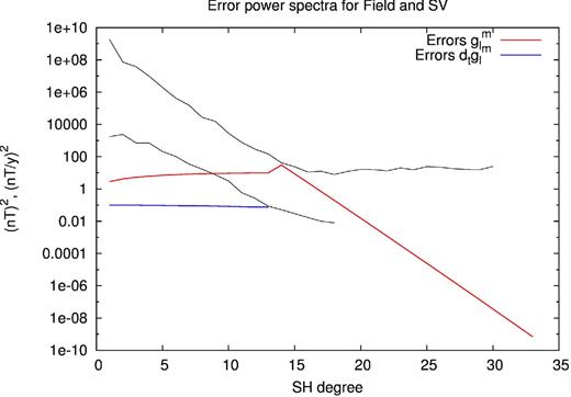
Black lines: power spectra at the Earth's surface of the magnetic field and its SV. Solid red line: estimated power of the error in core field models. At SH degrees larger than 13 it corresponds to a white spectrum at the CMB. For SH degrees 13 and below, the power corresponds to a theoretical spectrum for the lithosphere (Thébault & Vervelidou 2014). Solid blue line: estimated power of the error in SV models, assuming white noise at the Earth's surface.

We now turn to the starting models for the iterative process defined by eqs (17) and (18). Two starting models are required; one for the magnetic field, and one for the flow. The starting model for the field, called the G model, is obtained from the set of selected magnetic data presented at the beginning of this section, using eqs (11) and (12) only. An iterative process is used to estimate G with the weights defined in eq. (19), where a_j is set to 2 for the first iteration. We used the value λ_B = 1. This starting model for the field is therefore derived in a very similar way to the GRIMM series (Lesur et al.2008, 2010b; Mandea et al.2012). The starting model for the flow is derived using the first form of eqs (13) and (15). The magnetic field required to calculate A_B was defined by model G. Again, the weights are the same as those prescribed above, but the problem is linear. We used the value |$\lambda _U^T=10^{-3}$| for pure toroidal flows and |$\lambda _U^T=10^{-3}$| and |$\lambda _U^P=10$| for general flows.

Two models are outputs of the co-estimation processing scheme: the STG model for a pure toroidal flow and the SG model for a general flow (i.e. a combination of poloidal and toroidal flows). For these two models we used the value λ_B = 10⁻⁵, five orders of magnitude smaller than that used for the starting model because in a co-estimation approach the flow controls the field's temporal behaviour. The constraint applied on the field through eq. (12) is therefore effective only for the highest SH degrees of the core field model. The |$\lambda _U^T$| value is set to 10⁻³ and the |$\lambda _U^P$| value to 10. These are the same values as for the starting flow model. The parameter |$\tilde{\lambda }$| in eq. (16) is set to 70 for the general flow and to 2 × 10⁴ for the pure toroidal flow case. The latter relatively large |$\tilde{\lambda }$| value is a first indication of the difficulty in trying to reconcile a pure toroidal flow with satellite magnetic data.

4 RESULTS

We present in this section the main characteristics of the field and flow models obtained through our optimization process.

The G model is the starting field model for the co-estimation iterative process. As explained in the previous section, it has been derived using similar data selection, and the same constraints to control the temporal smoothness of the field, as the GRIMM series. Therefore, it shows similar features to the earlier GRIMM models. A snapshot of the field model and its SV are presented in Fig. 2. The field at the CMB shows the sinuous magnetic equator and the reverse patches of magnetic flux that have been present under the South Atlantic for at least 200 yr (e.g. Jackson et al.2000). The SV is relatively high in the western hemisphere (i.e. under Africa and the Atlantic Ocean) while it remains low under the Pacific Ocean and Antarctica (e.g. Holme et al.2011). The SA evolves very rapidly over the CHAMP era, closely matching that obtained in previous versions of the GRIMM model (see Fig. 3).

Figure 2.

Open in new tab Download slide

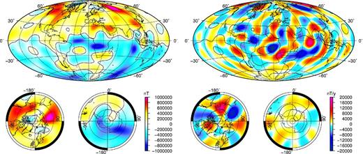
Vertically down components of the G model for 2005 at the CMB. Left-hand panel: the core field. Right-hand panel: the SV. In each case, below are polar cap images.

Figure 3.

Open in new tab Download slide

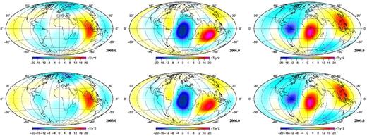
Vertically down component of the core field acceleration at the Earth's surface for the G model (top row) and the STG model (bottom row) at epochs 2003, 2006 and 2009.

The power spectra for the G model are shown in Fig. 4. As pointed out before, it is slightly more spatially smoothed than other models. This becomes evident in the steeper slope of the SA for SH degrees higher than 9. The fit to the data is given in Table 1, but it should be noted that the residuals present a distribution with large tails. Overall, there are no major differences between this model and other models derived from CHAMP satellite data.

Figure 4.

Open in new tab Download slide

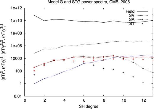
Power spectra of the G model (in black) and STG model (in red) for year 2005. The spectra are estimated at the CMB. SV and SA stand for secular variation and secular acceleration, respectively. ST is the third time derivative. The static and SV components of the model spectra cannot be distinguished. The spectrum of the SV differences is shown in blue.

The STG model is derived from a starting model that is updated during the co-estimation process, affecting both the (purely toroidal) flow and the field models. Changes in the field model are visible in the power spectrum of the SA that has more energy compared to the G model at SH degrees higher than 10 and in the power spectrum of the third time derivative that is generally higher (see Fig. 4). However, the field model remains very smooth in time. The STG model SV snap-shots for 2005 cannot be distinguished visually from those of the G model in Fig. 2. The modelled acceleration patterns are similar to those of the G model (see Fig. 3), although with slightly lower amplitudes in 2006.

The STG model fits the satellite data slightly worse than the G model (Table 1), but given the uncertainty on the true level of noise in the data, enhanced by the simplistic external field modelling, this misfit increase may not be significant. A map of the differences between G and STG model residuals (Fig. 5) nonetheless reveals that the misfit increase is particularly large over two areas, the Indian Ocean and central America, providing some indications of a failure of the pure toroidal flow hypothesis. We will return to this point in the next section.

Figure 5.

Open in new tab Download slide

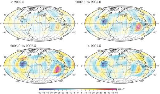
Differences between G and STG model residuals to the mid and low latitude X_SM satellite data, for four different time periods.

A snapshot in 2005 of the pure toroidal flow model, whose mean flow velocity is 12.6 km yr⁻¹, is plotted in Fig. 6, together with its spectra. The flow is strongly symmetric (78 per cent) and geostrophic (91.7 per cent), but its zonal toroidal component represents only 48.2 per cent of its total kinetic energy. Overall the main flow features described for example in Pais & Jault (2008) are all present.

Figure 6.

Open in new tab Download slide

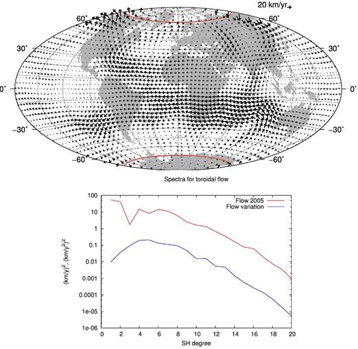
Top panel: estimated pure toroidal flow for the STG model, at the CMB and for 2005. The projection of the tangent cylinder on the Northern and Southern polar cap is highlighted in red. Bottom panel: estimated spectra for the flow and acceleration for 2005.

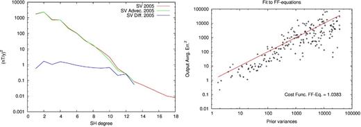
The fit to the induction equation is characterized by the mean-square difference between |$\mathbf {\dot{g}}$| predicted by the induction eq. (13) and from the field model according to eq. (14), weighted by the inverse of its covariance matrix |${\mathbf {C}}_{\dot{\mathbf {g}}}$| given by eq. (20). For the STG model, it has a value of 1.03, close to the target value of 1. This fit is illustrated by Fig. 7(left-hand panel), where the power spectra of the model SV for 2005, that of the SV generated through advection of the field by the flow, and of the differences between the two, are shown. Fig. 7(right-hand panel) presents the time averaged fit to the induction equation rotated using the eigenvectors of |${\mathbf {C}}_{\dot{\mathbf {g}}}$|⁠. In principle, these time averaged errors should lie close to the red line. In the present case, there is an obvious over-fit for small prior variances and a corresponding under-fit for large prior variance (the log-scale may slightly hide this under-fit).

Figure 7.

$Left-hand panel: power spectra at Earth's surface of the estimated SV, the advected SV and the difference between the two for the STG model. Right-hand panel: comparison between the fit to the time averaged induction equation rotated using the eigenvector of ${\mathbf {C}}_{\dot{\mathbf {g}}}$ and the eigenvalues of the same covariance matrix (20).$

Open in new tab Download slide

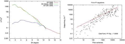
Left-hand panel: power spectra at Earth's surface of the estimated SV, the advected SV and the difference between the two for the STG model. Right-hand panel: comparison between the fit to the time averaged induction equation rotated using the eigenvector of |${\mathbf {C}}_{\dot{\mathbf {g}}}$| and the eigenvalues of the same covariance matrix (20).

The SG model, whose flow has both toroidal and poloidal parts, has been built to check that at least one flow model explaining the observed magnetic field exists. However, we have severely restricted the amount of poloidal flow by setting the scaling parameter |$\lambda _U^P$| four orders of magnitude larger than |$\lambda _U^T$|⁠. Hence the flow is almost toroidal, but has a small, essentially large-scale, poloidal component, which is plotted in Fig. 8 together with the flow spectra. This general flow has a mean flow velocity of 12.2 km yr⁻¹. Since the poloidal flow component contributes very little, the flow characteristics are virtually unchanged compared to the STG flow: the symmetric, geostrophic and zonal toroidal components represent 81.7 per cent, 92.5 per cent and 46.7 per cent of the kinetic energy respectively. The poloidal component itself represents only 0.4 per cent of the total kinetic energy.

Figure 8.

Open in new tab Download slide

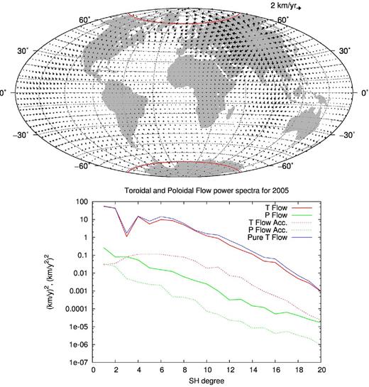
Top panel: estimated poloidal component of the SG flow at the CMB for 2005. Note the order of magnitude change in the length of the reference flow vector compared to Fig. 6. The projection of the tangent cylinder on the Northern and Southern polar cap is highlighted in red. Bottom panel: estimated spectra for the flow and its acceleration for 2005. The spectra in red are for the toroidal flow, in green for the poloidal flow, and in blue is shown the spectrum of the toroidal flow of the STG model.

The SG magnetic field model fits the selected mid-latitude satellite data significantly better than that of the STG model (see Table 1) but it has a rougher temporal behaviour. Smoothing the flow in time has no apparent effect on the magnetic field temporal roughness for the range of parameters we explored and, ultimately, we did not use such constraints. No areas with relatively high misfit to the data were identified. The weighted mean-square misfit to the induction equation is 1.04 compared to the target value of 1. The power spectra of the SG model SV and the advected SV for 2005 are shown in Fig. 9(left-hand panel). The time averaged fit to the induction equations rotated using the eigenvectors of |${\mathbf {C}}_{\dot{\mathbf {g}}}$| presented in Fig. 9(right-hand panel) is more homogeneous than for the STG model (i.e. the small prior variances are not over-fit as in Fig. 7). Overall this combination of poloidal and toroidal flow represents a model that fits both the data and the induction equation to within their error budget, without any biases in the data residuals.

Figure 9.

$Left-hand panel: power spectra of the estimated SV, the advected SV and the difference between the two for the SG model. Right-hand panel: comparison between the fit to the time averaged induction equation rotated using the eigenvector of ${\mathbf {C}}_{\dot{\mathbf {g}}}$ and the eigenvalues of the same covariance matrix.$

Open in new tab Download slide

Left-hand panel: power spectra of the estimated SV, the advected SV and the difference between the two for the SG model. Right-hand panel: comparison between the fit to the time averaged induction equation rotated using the eigenvector of |${\mathbf {C}}_{\dot{\mathbf {g}}}$| and the eigenvalues of the same covariance matrix.

5 DISCUSSION

In this study, we have built three models of the core magnetic field and several flow models, two of which are co-estimated with the field models. In all cases, the data set is identical and the starting weights used are the same. The weights evolve differently during the iterative reweighted least squares process for the different inversions, but the resulting models, their morphologies, temporal evolutions and fit to the data can be meaningfully compared.

Table 1 shows that, at high latitudes, the misfits to the three components of the magnetic field data are too large to be able to see the influence of SV generated by diffusion or by poloidal flow; this would also be the case if we computed and compared the fit to the total intensity (often preferred to vector component data at higher latitudes, since the scalar values are thought to be less contaminated by external fields). In contrast, at mid and low latitudes the noise level is very low. In the following we therefore focus on the mid latitude results. We recall that only the X_SM and Y_SM components are used for modelling the internal field and the prior rms misfits to these data components are nowadays below 3 nT. The G model therefore fits the data satisfactorily. The scaled histograms of residuals are presented in Fig. 10 and no major deviations from the prior distribution are observed. Finally, the spatial and temporal plots for these residuals do not reveal specific structures, other than the strongest lithospheric field anomalies that are not fully modelled with a maximum SH degree limited to 60 (not shown). As an example, the full set of X_SM and Y_SM residuals are displayed as a function of longitude in Fig. 11. They do not present unexpected large values. From this close investigation of the data residuals, the G model appears to be a good representation of the magnetic field measured at CHAMP altitude.

Figure 10.

Open in new tab Download slide

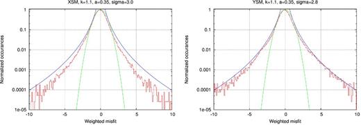
In red: histograms of residuals of the G model to the X_SM and Y_SM data. Histograms have been scaled such that they can be compared with their expected distributions. The Gaussian distribution is in green. In blue is the distribution corresponding to the weights in eq. (19). The differences between expected and final distributions remain small, even though the prior standard deviation for X_SM is probably slightly too large.

Figure 11.

Open in new tab Download slide

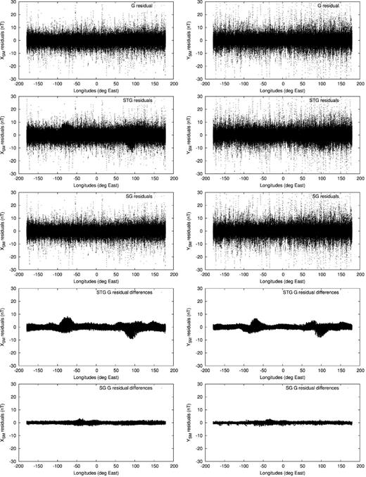
From top to bottom: residuals to the selected X_SM and Y_SM data for the G model, STG model and SG model, followed by the differences in residuals between the G and STG, and finally G and SG, models. Left-hand panel: X_SM component. Right-hand panel: Y_SM component.

Observatory data are not used in the modelling and therefore these data provide an independent set of measurements against which to test our models. The Chambon-la-Forêt (CLF), Hermanus (HER) and Kakioka (KAK) SV values, estimated following the method described in Wardinski & Holme (2006), are shown in Fig. 12 together with the SV estimated from the G model. Here again the fit to the data is remarkably good and is similar for all other observatories tested, confirming the quality of the G model.

Figure 12.

Open in new tab Download slide

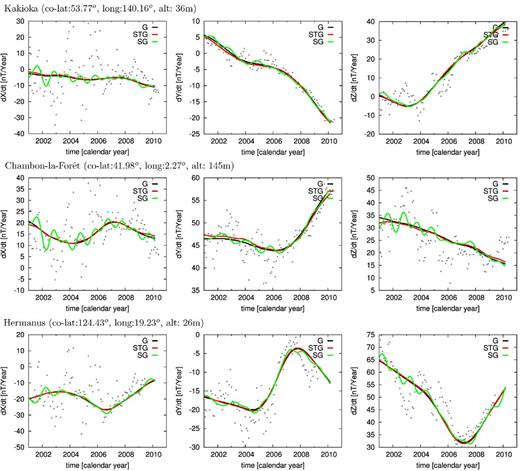
Estimated SV at three observatories (black dots) and calculated SV for the three models G, STG and SG in black, red and green, respectively.

As a final assessment, the model is compared with CHAOS-4 (Olsen et al.2014). Power spectra and the power spectrum of SV differences are shown in Fig. 13. The differences are small and therefore in the remainder of this paper the G model will be used as a reference for comparison with the co-estimated models.

Figure 13.

Open in new tab Download slide

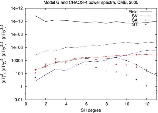
Power spectra of the G model (in black) and CHAOS-4 model (in red) for year 2005. The spectra are estimated at the CMB. SV and SA stand for secular variation and secular acceleration, respectively. ST is the third time derivative. The static and SV components of the models are indistinguishable. The spectrum of SV differences is shown in blue.

First, we consider the STG model. A comparison of the magnetic field power spectra of this model with the G model for year 2005 shows generally good agreement (see Fig. 4). The STG acceleration has more power at small wavelengths as is to be expected in the co-estimation approach (Lesur et al.2010a). It also has the same power as the G model at long wavelengths. This is surprising because it is barely smoothed in time – λ_B for the STG model is set to a value 10⁻⁵ smaller than in the G model. The temporal smoothness of the STG model is therefore imposed by the flow, because we demand a rapidly converging flow spectrum. We note that it would be difficult to generate a pure toroidal flow that leads to rough temporal variations of the large-scale field, without a significant increase of the flow kinetic energy at small-scales. This would clearly break the large-scale flow hypothesis. The STG model flow, shown in Fig. 6, is an adequate fit to the induction equation and has the usual flow geometry and spectrum; it is not significantly different from the starting model.

Although the overall fit to the data (Table 1) remains in the expected range, the residual differences shown in Fig. 5 are far from being uniformly distributed. The fit to the X_SM and Y_SM components is displayed in Fig. 11(second row) as well as the difference between the G and STG model residuals (fourth row). There are clusters of misfits at values of about 8 nT, well above the expected noise level in CHAMP data. These misfit anomalies are not static in time. The anomaly over the Indian Ocean slowly builds up from 2000 to reach a maximum in 2005, and vanishes before 2010, whereas that over central America intensifies from 2002 to reach a maximum amplitude in 2006 and decreases thereafter (see Fig. 5). Again, this is linked to the field model temporal behaviour, controlled by the flow, that is (locally) too smooth. We point out that the residual anomalies in Fig. 5 do not correspond in space and time to the strong acceleration patterns observed during the CHAMP era and displayed in Fig. 3 (see also for example Mandea et al.2012; Chulliat & Maus 2014; Olsen et al.2014). Finally, we note that the observatory distribution is not dense enough to provide an independent check on the results. In particular, there are no geomagnetic observatories in these areas of increased misfit and therefore the fit of the modelled SV to observatory estimates is acceptable (see Fig. 12).

The co-estimation process with a large scale pure toroidal flow leads therefore to a model that does not fit the satellite data everywhere to their expected level. We tried several starting models and regularization parameters without changing the final result: It is not possible to fit the data within the framework of our STG model. The comparison with the G model indicates that this behaviour is directly linked to the constraints generated by the flow and not due to poor modelling of the external fields. Unfortunately, we are not able to investigate flows with significant kinetic energy at small scales because the iterative scheme used to handle the SV covariance matrix would fail to converge (see Appendix B). If the large-scale flow hypothesis is dropped, the field model would not be constrained by the flow simply because there would be more degrees of freedom in the flow than in the field model. The satellite data would then be over-fit.

There are two points that needs to be clarified before going further in the discussion of the data misfit: first, is this a result of overfitting the induction equation, and second, is it possible to fit the data if the toroidal flow hypothesis is relaxed? The first point can be assessed by going back to eq. (B4) and Fig. 1. The spectrum for the error in the core field is white at the CMB for SH degrees between 13 and 33. This is less conservative than the extrapolated spectrum estimated by, for example, Voorhies (2004) and seems acceptable when compared to outputs of numerical dynamo models (e.g. Fig. 10 in Christensen et al.2012). At SH degrees lower than 13, the error spectrum is set to that of the lithospheric field, as this is the dominant error in the field model at these wavelengths. This latter point is supported by the spectrum of differences between the CHAOS and GRIMM field models that usually remains below the lithospheric spectrum, with possibly an exception at SH degree 1 that we will ignore here. We chose the lithospheric spectrum proposed by Thébault & Vervelidou (2014), other possible spectra (e.g. Jackson 1994) do not provide much larger error estimates. We set the spectrum of the error in the SV at 0.01 (nT yr⁻¹)⁻² as it corresponds roughly to the energy of the SV at SH degree 14, where the noise level of high latitude data starts to generate significant artefacts. We do not account here for diffusion processes in the core. We assume that the SV generated by diffusion remains weaker than the 0.01 (nT yr⁻¹)⁻² threshold, even if outputs of numerical dynamo models indicate much larger contributions (Amit & Christensen 2008; Aubert 2014). The main limitation in the way the error budget is set is the lack of correlation through assuming that the covariance matrices C_g and |$\mathbf {C_{\epsilon _s}}$| are diagonal. In particular, diffusion associated with flux expulsion may be localized (Bloxham 1988a) and therefore could locally generate SV stronger than the set threshold, leading to large off-diagonal elements in |$\mathbf {C_{\epsilon _s}}$|⁠. Outside possible localized effects of diffusion, we have accounted for the largest sources of errors in the magnetic field and SV. As found by other authors, the contribution of the small scale core field to the error budget appears to be very large, as shown in Fig. 7 where the spectrum of the difference between advected and modelled SV is more than one order of magnitude larger than the prior noise spectrum of the SV. We conclude that the SV generated by advection in the STG model is probably not over-fitting the modelled SV if the contribution from diffusion is small.

The second point has been tested by applying the same co-estimation approach to a general flow. We did not aim here to build the most realistic flow model, but simply to demonstrate that we can generate a model, referred to as SG, with minimal poloidal flow (by damping heavily that part relative to the toroidal flow) whose associated field model fits the satellite data to their expected level and without bias. The misfit to the data, presented in Table 1, is lower than that of the G model. There is a risk here that the model overfits the data and that a small part of the external field has leaked into the core field model. This seems to be confirmed by the relatively large values of the third time derivative spectrum of the SG model (not shown), which indicate rapid variations of the SA that are suspicious even if there are no theoretical arguments to reject such behaviour. These variations are also visible in the predictions of observatory SV data in Fig. 12. Oscillations occur in all components and are particularly large in the north (i.e. |$\dot{X}$|⁠) component. The residuals to the data are presented in Fig. 11, which show no regional anomalies. Similarly, the histograms of data residuals do not indicate any anomalies. The induction equation is fit to its expected level. The flow is dominated by its toroidal component that is difficult to distinguish from the STG model flow. It has nonetheless slightly less kinetic energy and a small, but large-scale, poloidal component dominated by an upwelling under Siberia. We conclude that the SG model is acceptable in some of its characteristics, but is too rough in time. Despite of the strong constraints we applied to the poloidal flow, the number of degrees of freedom introduced (mainly at large scales) is so large that the flow does not control the SV and acceleration of the magnetic field model effectively, which over-fits the satellite data. This could be corrected by applying stronger temporal smoothing constraints directly on the field, or by limiting further the poloidal flow energy. Overall the SG model establishes that there is a general flow compatible with the observed magnetic field, unlike the situation for a large-scale pure toroidal flow.

It is tempting to suggest that a large-scale pure toroidal flow could also be compatible with the observed magnetic field if diffusion was accounted for in the modelling effort. However, diffusion has time scales much longer than the observed field evolution, and the anomalous misfit of the STG model to the satellite data evolves rapidly in time. Further, dealing with diffusion by introducing a larger uncorrelated error budget for the SV is unlikely to give meaningful results since setting too relaxed an error bound leads, as in the SG model, to a solution where the field model is not sufficiently controlled by the flow. Assimilation methods allow for much stronger constraints on the SV generated by diffusion because the diffusive SV is controlled by the deep structure of the field and the flow. As used for example by Fournier et al. (2011) and Aubert (2014), these methods lead to covariance matrices C_g and |$\mathbf {C_{\epsilon _s}}$|⁠, in eqs (21) and (B4), that are not diagonal. We suggest that a definitive test of the stratification hypothesis is more likely to come from using such assimilation techniques on satellite data. Nonetheless numerical dynamo models have first to be run in the correct dynamic regime.

There is a remaining risk that the results we obtain here arise from having a relatively short data time span. Although unlikely, it is still possible that the fast evolution of the anomalous misfit to satellite data in the STG model is due to edge effects. A longer duration study based on a combined CHAMP and current Swarm mission data set may resolve this issue.

Finally, we reiterate that the SG model has been derived simply to demonstrate that an acceptable co-estimated flow and field model exists. It is not envisaged as a realistic model of the flow, simply one of a large set of models compatible with the data. We expected that its poloidal component would be relatively small-scale, concentrated in areas of anomalously large data misfit for the STG model, but this is not what resulted. Instead, the flow obtained shows similarities with the results of Jault & Le Mouël (1991), who demonstrated that the large scale component of a stratified flow is likely to remain tangentially geostrophic, and therefore have only a small amount of large scale poloidal flow, while the smaller scales of the flow tend to be purely toroidal. Thus, although we have shown that a large scale, purely toroidal flow is not reconcilable with the observed magnetic field, the possibility of weak stratification compatible with a large scale poloidal flow prevents us from concluding definitively that the hypothesis of stratified flow at the top of the core must fail.

6 CONCLUSION

We tested the hypothesis of stratification of the top of the core by attempting to verify that a large-scale pure toroidal flow is compatible with the observed magnetic field during the CHAMP era. We built a series of co-estimated magnetic field and flow models, allowing us to test directly the flow hypothesis on the observed data. We put significant effort into setting realistic error budgets on the induction equation, to conclude ultimately that for an essentially large-scale pure toroidal flow, we cannot fit the CHAMP satellite data to their expected noise level. However, we are not able to conclude that this violates the hypothesis that the upper reaches of the outer core are stably stratified, because a small amount of large-scale poloidal flow would still be compatible with it, and we have found at least one model fitting the satellite data under this condition. Further our result assumes little or no SV is generated by diffusion of the magnetic field. A small amount of SV generated locally by diffusion may lead to an acceptable fit to the data under a large-scale pure toroidal flow hypothesis.

Our results nonetheless show the importance of time dependence in the field and flow modelling. We would have been unable to test the toroidal flow hypothesis on a simple snapshot model. Imposing the constraint that the SV is generated by a large scale pure toroidal flow leads to field models that are too smooth in time and therefore unable to follow the evolution of the magnetic field as observed by the CHAMP satellite. With the continuously improving quality of observatory data and the accumulation of satellite data, it is important to establish realistic bounds on the time dependence of the flow and/or Gauss coefficients in order to progress further in our understanding of core structure and dynamics.

We would like to acknowledge the work of the CHAMP satellite processing team and of the scientists working in magnetic observatories. We also thank two anonymous reviewers for their comments that certainly helped in improving the manuscript. Maps have been produced using GMT scripts (Wessel & Smith 1991).

REFERENCES

Abramowitz

M.

,

Stegun

I.A.

. ,

Handbook of Mathematical Functions

,

1964

Dover Press

Google Scholar

Google Preview

OpenURL Placeholder Text

WorldCat

Amit

H.

,

Christensen

U.

.

Accounting for magnetic diffusion in core flow inversions from geomagnetic secular variation

,

Geophys. J. Int.

,

2008

, vol.

175

(pg.

913

-

924

)

Aubert

J.

.

Earth's core internal dynamics 1840–2010 imaged by inverse geodynamo modelling

,

Geophys. J. Int.

,

2014

, vol.

197

3

(pg.

1321

-

1334

)

Backus

G.E.

.

Kinematics of geomagnetic secular variation in a perfectly conducting core

,

Phil. Trans. R. Soc. Lond., A

,

1968

, vol.

263

(pg.

239

-

266

)

Backus

G.

,

Parker

R.

,

Constable

C.

. ,

Foundations of Geomagnetism

,

1996

Cambridge Univ. Press

Google Scholar

Google Preview

OpenURL Placeholder Text

WorldCat

Baerenzung

J.

,

Holschneider

M.

,

Lesur

V.

.

Bayesian inversion of the filtered flow at the Earth's core mantle boundary

,

J. geophys. Res.: Solid Earth

,

2014

, vol.

119

4

(pg.

2695

-

2720

)

Bloxham

J.

.

The dynamical regime of fluid flow at the core surface

,

Geophys. Res. Lett.

,

1988a

, vol.

15

(pg.

585

-

588

)

Bloxham

J.

.

Vlaar

N.J.

,

Nolet

G.

,

Wortel

M.J.R.

,

Cloetingh

S.A.P.L.

.

The determination of fluid flow at the core surface from geomagnetic observations

,

Mathematical Geophysics, A Survey of Recent Developments in Seismology and Geodynamics

,

1988b

Reidel

(pg.

189

-

208

)

Google Scholar

Google Preview

OpenURL Placeholder Text

WorldCat

Bloxham

J.

.

On the consequences of strong stable stratification at the top of the Earth's outer core

,

Geophys. Res. Lett.

,

1990

, vol.

17

(pg.

2081

-

2084

)

Christensen

U.

,

Wardinski

I.

,

Lesur

V.

.

Time scales of geomagnetic secular acceleration in satellite field models and geodynamo models

,

Geophys J. Int.

,

2012

, vol.

190

(pg.

243

-

254

)

Chulliat

A.

,

Maus

S.

.

Geomagnetic secular acceleration, jerks, and a localized standing wave at the core surface from 2000 to 2010

,

J. geophys. Res.: Solid Earth

,

2014

, vol.

119

3

(pg.

1531

-

1543

)

Farquharson

C.

,

Oldenburgh

D.

.

Non-linear inversion using general measures of data misfit and model structure

,

Geophys. J. Int.

,

1998

, vol.

134

(pg.

213

-

227

)

Fournier

A.

,

Aubert

J.

,

Thébault

E.

.

Inference on core surface flow from observations and 3-D dynamo modelling

,

Geophys. J. Int.

,

2011

, vol.

186

1

(pg.

118

-

136

)

Gibson

R.

,

Roberts

P.H.

.

Runcorn

S.

.

The Bullard-Gellman dynamo, in

,

Applications of Modern Physics to the Earth and Planetary Interiors

,

1969

Wiley-Interscience

(pg.

577

-

602

)

Google Scholar

Google Preview

OpenURL Placeholder Text

WorldCat

Gubbins

D.

.

A formalism for the inversion of geomagnetic data for core motions with diffusion

,

Phys. Earth planet Inter.

,

1996

, vol.

98

(pg.

193

-

206

)

Gubbins

D.

,

Davies

C.

.

The stratified layer at the core–mantle boundary caused by barodiffusion of oxygen, sulphur and silicon

,

Phys. Earth planet. Inter.

,

2013

, vol.

215

(pg.

21

-

28

)

Helffrich

G.

,

Kaneshima

S.

.

Outer-core compositional stratification from observed core wave speed profiles

,

Nature

,

2010

, vol.

468

(pg.

807

-

810

)

Holme

R.

.

Olson

P.

.

Large-scale flow in the core, in

,

Treatise on Geophysics

,

2007

, vol.

8

Elsevier Ltd

Vol

Google Scholar

Google Preview

OpenURL Placeholder Text

WorldCat

Holme

R.

,

Olsen

N.

,

Braistow

F.

.

Mapping geomagnetic secular variation at the core-mantle boundary

,

Geophys J. Int.

,

2011

, vol.

186

2

(pg.

521

-

528

)

Hulot

G.

,

Le Mouël

J.L.

,

Wahr

J.

.

Taking into account the truncation problems and geomagnetic model accuracy in assessing the computed flow at the core-mantle boundary

,

Geophys. J. Int.

,

1992

, vol.

108

(pg.

224

-

246

)

Hulot

G.

,

Olsen

N.

,

Thébault

E.

,

Hemant

K.

.

Crustal concealing of small scale core field secular variation

,

Geophys. J. Int.

,

2009

, vol.

177

(pg.

361

-

366

)

Jackson

A.

.

Statistical treatment of crustal magnetization

,

Geophys. J. Int.

,

1994

, vol.

119

(pg.

991

-

998

)

Jackson

A.

.

Time-dependency of tangentially geostrophic core surface motions

,

Phys. Earth planet. Inter.

,

1997

, vol.

103

(pg.

293

-

311

)

Jackson

A.

,

Finlay

C.

.

Shubert

G.

.

Geomagnetic secular variation and applications to the core, in

,

Treatise on Geophysics

,

2007

Elsevier Ltd.

Vol. 5

Google Scholar

Google Preview

OpenURL Placeholder Text

WorldCat

Jackson

A.

,

Jonkers

A.R.T.

,

Walker

M.R.

.

Four centuries of geomagnetic secular variation from historical records

,

Phil. Trans. R. Soc. Lond., A

,

2000

, vol.

358

(pg.

957

-

990

)

Jault

D.

,

Le Mouël

J.L.

.

Physical properties at the top of the core and core surface motions

,

Phys. Earth planet. Inter.

,

1991

, vol.

68

(pg.

76

-

84

)

Kunagu

P.

,

Balasis

G.

,

Lesur

V.

,

Chandrasekhar

E.

.

wavelet characterization of the external magnetic sources as observed by CHAMP satellite: evidence for unmodelled signals in geomagnetic field models

,

Geophys. J. Int.

,

2013

, vol.

192

3

(pg.

946

-

950

)

Lesur

V.

,

Wardinski

I.

,

Rother

M.

,

Mandea

M.

.

GRIMM—the GFZ reference internal magnetic model based on vector satellite and observatory data

,

Geophys. J. Int.

,

2008

, vol.

173

2

(pg.

382

-

394

)

Lesur

V.

,

Wardinski

I.

,

Asari

S.

,

Minchev

B.

,

Mandea

M.

.

Modelling the Earth's core magnetic field under flow constraints

,

Earth, Planets Space

,

2010a

, vol.

62

(pg.

503

-

516

)

Lesur

V.

,

Wardinski

I.

,

Hamoudi

M.

,

Rother

M.

.

The second generation of the GFZ reference internal magnetic field model: GRIMM-2

,

Earth Planets Space

,

2010b

, vol.

62

10

(pg.

765

-

773

)

Lesur

V.

,

Rother

M.

,

Vervelidou

F.

,

Hamoudi

M.

,

Thébault

E.

.

Post-processing scheme for modelling the lithospheric magnetic field

,

Solid Earth

,

2013

, vol.

4

(pg.

105

-

118

)

Love

J.J.

.

A critique of frozen-flux inverse modelling of a nearly steady geodynamo

,

Geophys. J. Int.

,

1999

, vol.

138

(pg.

353

-

365

)

Mandea

M.

,

Panet

I.

,

Lesur

V.

,

De Viron

O.

,

Diament

M.

,

Le Mouël

J.L.

.

The Earth's fluid core: recent changes derived from space observations of geopotential fields

,

PNAS

,

2012

, vol.

109

47

(pg.

19 129

-

19 133

)

Maus

S.

,

Lühr

H.

.

Signature of the quiet-time magnetospheric magnetic field and its electromagnetic induction in the rotating earth

,

Geophys. J. Int.

,

2005

, vol.

162

(pg.

755

-

763

)

Maus

S.

,

Weidelt

P.

.

Separating the magnetospheric disturbance magnetic field into external and transient internal contributions using a 1D conductivity model of the Earth

,

Geophys. Res. Lett.

,

2004

, vol.

31

pg.

L12614

10.1029/2004GL020232

Google Scholar

OpenURL Placeholder Text

WorldCat

Crossref

Olsen

N.

,

Sabaka

T.

,

Lowes

F.

.

New parameterisation of external and induced fields in geomagnetic field modelling, and a candidate model for IGRF 2005

,

Earth Planets Space

,

2005

, vol.

57

(pg.

1141

-

1149

)

Olsen

N.

,

Lühr

H.

,

Finlay

C.

,

Sabaka

T.J.

,

Michaelis

I.

,

Rauberg

J.

,

Tøffner-Clausen

L.

.

The CHAOS-4 geomagnetic field model

,

Geophys. J. Int.

,

2014

, vol.

197

2

(pg.

815

-

827

)

Pais

M.

,

Jault

D.

.

Quasi-geostrophic flows responsible for the secular variation of the Earth's magnetic field

,

Geophys. J. Int.

,

2008

, vol.

173

(pg.

421

-

443

)

Pozzo

M.

,

Davies

C.

,

Gubbins

D.

,

Alfè

D.

.

Thermal and electrical conductivity of iron at Earth's core conditions

,

Nature

,

2012

, vol.

485

(pg.

355

-

358

)

Roberts

P.H.

,

Scott

S.

.

On the analysis of secular variation, 1. A hydromagnetic constraint: theory

,

J. Geomag. Geoelectr.

,

1965

, vol.

17

(pg.

137

-

151

)

Thébault

E.

,

Vervelidou

F.

.

A statistical spatial power spectrum of the Earth's lithospheric magnetic field

,

Geophys. J. Int.

,

2014

in press

Google Scholar

OpenURL Placeholder Text

WorldCat

Thomson

A.

,

Lesur

V.

.

An improved geomagnetic data selection algorithm for global geomagnetic field modelling

,

Geophys. J. Int.

,

2007

, vol.

169

(pg.

951

-

963

)

Voorhies

C.V.

.

Narrow-scale flow and a weak field by the top of Earth's core: evidence from Ørsted, Magsat, and secular variation

,

J. geophys. Res.

,

2004

, vol.

109

pg.

B03106

Wardinski

I.

,

Holme

R.

.

A time-dependent model of the Earth's magnetic field and its secular variation for the period 1980 to 2000

,

J. geophys. Res.

,

2006

, vol.

111

pg.

B12101

Wessel

P.

,

Smith

W. H.F.

.

Free software helps map and display data

,

EOS, Trans. Am. geophys. Un.

,

1991

, vol.

72

(pg.

445

-

446

)

441 &

Whaler

K.A.

.

Does the whole of the Earth's core convect?

,

Nature

,

1980

, vol.

287

(pg.

528

-

530

)

Whaler

K.A.

.

Fluid upwelling at the core-mantle boundary—resolvability from surface geomagnetic data

,

Geophys. J.

,

1984

, vol.

78

(pg.

453

-

473

)

Whaler

K.A.

.

Geomagnetic evidence for fluid upwelling at the core-mantle boundary

,

Geophys. J. R. astr. Soc.

,

1986

, vol.

86

(pg.

563

-

588

)

APPENDIX A: FILTERED INDUCTION EQUATION

We follow here the same developments and approximations as in Baerenzung et al. (2014) to write the induction equation for smoothed magnetic field, SV and flow. This is achieved in eqs (A8) and (A10). From there, no further approximations are made, but rather tedious developments are presented to obtain the equations in the SH domain for both pure poloidal flows (eq. A25) and pure toroidal flows (eq. A33) cases. To simplify the notation, we assume that the differential operators on the sphere, denoted ∇_h and Δ_h, are defined on the sphere of radius unity. Δ_h is the horizontal Laplacian, sometimes referred to as the angular momentum operator.

Baerenzung et al. (2014) have shown that convolving any function of space and time f(θ, ϕ, t) with a smoothing Gaussian filter is equivalent to letting the function evolve under the diffusion equation

\begin{equation} \Delta _h f(\theta ,\phi ,t) = \frac{1}{k} \partial _t f(\theta ,\phi ,t), \end{equation}

(A1)

where f(θ, ϕ, t) at t = 0 is the original function, k a diffusion coefficient, and f(θ, ϕ, t) is the smoothed function when t > 0. Therefore on a sphere of radius c the approximation

\begin{equation} f(\theta ,\phi ,t) \approx f(\theta ,\phi ,t^{\prime }) + (t-t^{\prime }) \partial _t f(\theta ,\phi ,t) |_{t=t^{\prime }}, \end{equation}

(A2)

leads for t^′ = 0 to

\begin{equation} f(\theta ,\phi ,t) \approx f(\theta ,\phi ,0) + \frac{kt}{c^2} \Delta _h f(\theta ,\phi ,0). \end{equation}

(A3)

This shows that we can approximate a smoothed version of a function by the function itself using the Δ_h operator. Similarly it is possible to approximate a function by its smoothed version by setting t = 0 in eq. (A2) and using eq. (A1)

\begin{equation} f(\theta ,\phi ,0) \approx f(\theta ,\phi ,t^{\prime }) - \frac{kt^{\prime }}{c^2} \Delta _h f(\theta ,\phi ,t^{\prime }). \end{equation}

(A4)

Applying these approximations to the radial component of the magnetic field B_r(θ, ϕ) and its smoothed version |$\tilde{B}_r(\theta ,\phi )$| gives:

\begin{eqnarray} \tilde{B}_r(\theta ,\phi ) \approx B_r(\theta ,\phi ) + \frac{kt}{c^2} \Delta _h B_r(\theta ,\phi ), \end{eqnarray}

(A5)

\begin{eqnarray} B_r(\theta ,\phi ) \approx \tilde{B}_r(\theta ,\phi ) - \frac{kt}{c^2} \Delta _h \tilde{B}_r(\theta ,\phi ). \end{eqnarray}

(A6)

The flow U_h and the product U_hB_r satisfy similar equations. Turning now to the radial component of the diffusion-less induction equation we have

\begin{equation} \partial _t B_r(\theta ,\phi ,t) = - \frac{1}{c} \nabla _h \cdot ({\mathbf {U}}_h B_r). \end{equation}

(A7)

By filtering this equation we obtain

\begin{equation} \partial _t \tilde{B}_r(\theta ,\phi ,t) = - \frac{1}{c} \nabla _h \cdot {(\tilde{\mathbf {U}}_h \tilde{B}_r)} - \frac{1}{c} \nabla _h \cdot {\tau }, \end{equation}

(A8)

where τ is given by

\begin{equation} {\tau } = \tilde{({\mathbf {U}}_h B_r)} - \big(\tilde{\mathbf {U}}_h \tilde{B}_r\big). \end{equation}

(A9)

Let us set |$\lambda = \frac{kt}{c^2}$|⁠. By using an equation equivalent to (A5) for the product |$\tilde{{\mathbf {U}}_hB_r}$| and then after, eq. (A6) and its equivalent for the flow U_h, we obtain

\begin{equation} {\tau} \approx \lambda \; \big[ \Delta _h \big(\tilde{\mathbf {U}}_h \tilde{B}_r\big) - \tilde{B}_r \Delta _h \tilde{\mathbf {U}}_h - \tilde{\mathbf {U}}_h \Delta _h \tilde{B}_r \big], \end{equation}

(A10)

where all terms in λ of order 2 and higher have been neglected. Baerenzung et al. (2014) further reduce this expression to

\begin{equation} {\tau } = 2 \; \lambda \; \left( \nabla _h \tilde{B}_r \cdot \nabla _h \right) \tilde{\mathbf {U}}_h, \end{equation}

(A11)

but in view of a representation in spherical harmonics, it is easier to derive an expression for ∇_h · τ. We note first that

\begin{equation} \begin{array}{l}\nabla _h \cdot {\big(\Delta _h \big({\tilde{\mathbf {U}}}_h {\tilde{B}}_r\big)\big)} = \Delta _h \big( {\tilde{\mathbf {U}}}_h \cdot \nabla _h {\tilde{B}}_r\big) + {\tilde{B}}_r \Delta _h \big(\nabla _h \cdot {\tilde{\mathbf {U}}}_h\big) + \Delta _h {\tilde{B}}_r \big(\nabla _h \cdot {\tilde{\mathbf {U}}}_h\big) + 2 \nabla _h {\tilde{B}}_r \cdot \nabla _h \big(\nabla _h \cdot {\tilde{\mathbf {U}}}_h\big), \end{array} \end{equation}

(A12)

\begin{equation} \begin{array}{l}\nabla _h \cdot {\big({\tilde{\mathbf {U}}}_h \Delta _h {\tilde{B}}_r\big)} = {\tilde{\mathbf {U}}}_h \cdot \nabla _h \big(\Delta _h {\tilde{B}}_r\big) + \Delta _h {\tilde{B}}_r \big(\nabla _h \cdot {\tilde{\mathbf {U}}}_h\big), \end{array} \end{equation}

(A13)

\begin{equation} \begin{array}{l}\nabla _h \cdot {\big( {\tilde{B}}_r \Delta _h {\tilde{\mathbf {U}}}_h \big)} = \nabla _h {\tilde{B}}_r \cdot \nabla _h \big(\nabla _h \cdot {\tilde{\mathbf {U}}}_h\big) - \nabla _h {\tilde{B}}_r \cdot \nabla _h \times \big(\nabla _h \times {\tilde{\mathbf {U}}}_h\big) + {\tilde{B}}_r \Delta _h \big(\nabla _h \cdot {\tilde{\mathbf {U}}}_h\big), \end{array} \end{equation}

(A14)

which, from eq. (A10), leads to

\begin{equation} \nabla _h \cdot {\tau } = \lambda \; \left[\Delta _h ( {\tilde{\mathbf {U}}}_h \cdot \nabla _h {\tilde{B}}_r) + \nabla _h {\tilde{B}}_r \cdot (\nabla _h (\nabla _h \cdot {\tilde{\mathbf {U}}}_h) + \nabla _h \times (\nabla _h \times {\tilde{\mathbf {U}}}_h)) - {\tilde{\mathbf {U}}}_h \cdot \nabla _h \left(\Delta _h {\tilde{B}}_r\right)\right]. \end{equation}

(A15)

A1 Poloidal flow

Assuming the flow |${\tilde{\mathbf {U}}_h}$| is purely poloidal, it can be written as a function of a scalar field S:

\begin{equation} {\tilde{\mathbf {U}}}_h = \nabla _h{S}. \end{equation}

(A16)

Eq. (A15) then reduces to

\begin{equation} \nabla _h \cdot {{\tau }} = \lambda \; [\Delta _h ( \nabla _h {S} \cdot \nabla _h {\tilde{B}}_r) + \nabla _h {\tilde{B}}_r \cdot \nabla _h (\Delta _h S) - \nabla _h {S} \cdot \nabla _h (\Delta _h {\tilde{B}}_r)]. \end{equation}

(A17)

With the Gauss coefficients and the flow coefficients also defined on a sphere of radius c, the expressions for the radial component of the field, the poloidal scalar and their respective Laplacians are

\begin{eqnarray} {\tilde{B}}_r= \sum _{l,m} (l+1) g_l^m Y_l^m(\theta ,\phi ), \qquad & \Delta _h {\tilde{B}}_r= - \displaystyle\sum _{l,m} l(l+1)^2 g_l^m Y_l^m(\theta ,\phi ), \end{eqnarray}

(A18)

\begin{eqnarray} S= \sum _{l,m} s_l^m Y_l^m(\theta ,\phi ), \qquad& \Delta _h S = - \displaystyle\sum _{l,m} l(l+1) s_l^m Y_l^m(\theta ,\phi ). \end{eqnarray}

(A19)

Eq. (A17) becomes

\begin{equation} \begin{array}{r}\nabla _h \cdot {\tau } = \lambda \; \displaystyle\sum _{l,m,l^{\prime },m^{\prime }} (l+1) g_l^m s_{l^{\prime }}^{m^{\prime }} \; \left[ \; \Delta _h \left( \nabla _h Y_{l}^{m} \cdot \nabla _h Y_{l^{\prime }}^{m^{\prime }}\right) - l^{\prime } (l^{\prime }+1) \left( \nabla _h Y_{l}^{m} \cdot \nabla _h Y_{l^{\prime }}^{m^{\prime }}\right) + l(l+1) \left( \nabla _h Y_{l}^{m} \cdot \nabla _h Y_{l^{\prime }}^{m^{\prime }}\right) \; \right]. \end{array} \end{equation}

(A20)

We recall here the definition of the Gaunt integral (e.g. Gibson & Roberts 1969)

\begin{equation} G_{l,m,l^{\prime },m^{\prime }}^{l^{\prime \prime },m^{\prime \prime }}= \int _{\Omega _c} Y_{l}^{m} Y_{l^{\prime }}^{m^{\prime }} Y_{l^{\prime \prime }}^{m^{\prime \prime }} \; {\rm d}\omega , \end{equation}

(A21)

and we note that

\begin{equation} \int _{\Omega _c} \left(\nabla _h Y_{l}^{m} \cdot \nabla _h Y_{l^{\prime }}^{m^{\prime }}\right) Y_{l^{\prime \prime }}^{m^{\prime \prime }} \; {\rm d}\omega =\frac{1}{2} \; [ l(l+1) + l^{\prime }(l^{\prime }+1) - l^{\prime \prime }(l^{\prime \prime }+1) ] \;G_{l,m,l^{\prime },m^{\prime }}^{l^{\prime \prime },m^{\prime \prime }} \end{equation}

(A22)

\begin{equation} \int _{\Omega _c} \Delta _h \left(\nabla _h Y_{l}^{m} \cdot \nabla _h Y_{l^{\prime }}^{m^{\prime }}\right) Y_{l^{\prime \prime }}^{m^{\prime \prime }} \; {\rm d}\omega = - \frac{1}{2} \; [ l(l+1) + l^{\prime }(l^{\prime }+1) - l^{\prime \prime }(l^{\prime \prime }+1) ] l^{\prime \prime }(l^{\prime \prime }+1) \;G_{l,m,l^{\prime },m^{\prime }}^{l^{\prime \prime },m^{\prime \prime }} \end{equation}

(A23)

Multiplying both sides of eq. (A20) by |$Y_{l^{\prime \prime }}^{m^{\prime \prime }}$| and integrating over the sphere Ω_c gives

\begin{equation} \int _{\Omega _c} (\nabla _h \cdot {\tau })\, Y_{l^{\prime \prime }}^{m^{\prime \prime }} \; {\rm d}\omega =-\frac{\lambda }{2} \; \sum _{l,m,l^{\prime },m^{\prime }} (l+1) g_l^m s_{l^{\prime }}^{m^{\prime }} \; [ l(l+1) + l^{\prime }(l^{\prime }+1) - l^{\prime \prime }(l^{\prime \prime }+1) ] [ l^{\prime \prime }(l^{\prime \prime }+1) + l^{\prime }(l^{\prime }+1) - l(l+1) ] \;G_{l,m,l^{\prime },m^{\prime }}^{l^{\prime \prime },m^{\prime \prime }}. \end{equation}

(A24)

Consequently, the filtered diffusion-less induction equation in the SH domain for pure poloidal flow is

\begin{equation} \dot{g}_{l^{\prime \prime }}^{m^{\prime \prime }}=\frac{(2l^{\prime \prime }+1)}{8 \pi c (l^{\prime \prime }+1)} \; \sum _{l,m,l^{\prime },m^{\prime }} (l+1) g_l^m s_{l^{\prime }}^{m^{\prime }} \; [ 1+\lambda \lbrace l(l+1) + l^{\prime }(l^{\prime }+1) - l^{\prime \prime }(l^{\prime \prime }+1) \rbrace ] [ l^{\prime \prime }(l^{\prime \prime }+1) + l^{\prime }(l^{\prime }+1) - l(l+1) ] \;G_{l,m,l^{\prime },m^{\prime }}^{l^{\prime \prime },m^{\prime \prime }}. \end{equation}

(A25)

A2 Toroidal flow

Assuming the flow |${\tilde{\mathbf {U}}}_h$| is now purely toroidal, it can be written as a function of a scalar field T, such that

\begin{equation} {\tilde{\mathbf {U}}}_h= \nabla _h \times (\hat{{\mathbf {r}}}T), \end{equation}

(A26)

where |$\hat{{\mathbf {r}}}$| is the unit vector in the radial direction. Using |$\nabla _h \times (\hat{{\mathbf {r}}}T) = - \hat{{\mathbf {r}}} \times \nabla _h T$| we derive from eq. (A15)

\begin{eqnarray} \nabla _h \cdot {{\tau }} &=& \lambda \; \left[\Delta _h ( \nabla _h \times (\hat{{\mathbf {r}}}T) \cdot \nabla _h {\tilde{B}}_r) + \nabla _h {\tilde{B}}_r \cdot (\nabla _h \times \nabla _h \times \nabla _h \times (\hat{{\mathbf {r}}}T)) - \nabla _h \times (\hat{{\mathbf {r}}}T)\cdot \nabla _h (\Delta _h {\tilde{B}}_r)\right]\nonumber\\ &=& \lambda \; \left[\Delta _h ( \nabla _h \times (\hat{{\mathbf {r}}}T) \cdot \nabla _h {\tilde{B}}_r) - \nabla _h {\tilde{B}}_r \cdot (\nabla _h \times (\hat{{\mathbf {r}}} \Delta _h T)) - \nabla _h \times (\hat{{\mathbf {r}}}T)\cdot \nabla _h (\Delta _h {\tilde{B}}_r)\right]. \end{eqnarray}

(A27)

Again, the flow coefficients are defined on a sphere of radius c, and the toroidal scalar and its Laplacian are

\begin{equation} T= \sum _{l,m} t_l^m Y_l^m(\theta ,\phi ), \qquad \Delta _h T = - \sum _{l,m} l(l+1) t_l^m Y_l^m(\theta ,\phi ). \end{equation}

(A28)

Hence it follows that

\begin{equation} \nabla _h \cdot {{\tau }} = \lambda \; \sum _{l,m,l^{\prime },m^{\prime }} (l+1) g_l^m t_{l^{\prime }}^{m^{\prime }} \; \big[ \; \Delta _h \big( \nabla _h Y_{l}^{m} \cdot \nabla _h \times \big(\hat{{\mathbf {r}}} Y_{l^{\prime }}^{m^{\prime }}\big)\big) + l^{\prime }(l^{\prime }+1) \big( \nabla _h Y_{l}^{m} \cdot \nabla _h \times \big(\hat{{\mathbf {r}}} Y_{l^{\prime }}^{m^{\prime }}\big)\big) + l(l+1) \big( \nabla _h Y_{l}^{m} \cdot \nabla _h \times \big(\hat{{\mathbf {r}}} Y_{l^{\prime }}^{m^{\prime }}\big)\big) \; \big]. \end{equation}

(A29)

Elsasser's integral is defined by (Gibson & Roberts 1969)

\begin{equation} E_{l,m,l^{\prime },m^{\prime }}^{l^{\prime \prime },m^{\prime \prime }} = - \int _{\Omega _c} \left(\nabla _h Y_{l}^{m} \cdot \nabla _h \times \left(\hat{{\mathbf {r}}} Y_{l^{\prime }}^{m^{\prime }}\right)\right) Y_{l^{\prime \prime }}^{m^{\prime \prime }} \; {\rm d}\omega , \end{equation}

(A30)

and it can be shown that

\begin{equation} \int _{\Omega _c} \Delta _h \big(\nabla _h Y_{l}^{m} \cdot \nabla _h \times \big(\hat{{\mathbf {r}}} Y_{l^{\prime }}^{m^{\prime }}\big)\big) Y_{l^{\prime \prime }}^{m^{\prime \prime }} \; {\rm d}\omega = l^{\prime \prime }(l^{\prime \prime }+1) E_{l,m,l^{\prime },m^{\prime }}^{l^{\prime \prime },m^{\prime \prime }}. \end{equation}

(A31)

Therefore, multiplying both sides of eq. (A29) by |$Y_{l^{\prime \prime }}^{m^{\prime \prime }}$| and integrating over the sphere Ω_c gives:

\begin{equation} \int _{\Omega _c} (\nabla _h \cdot {{\tau }})\, Y_{l^{\prime \prime }}^{m^{\prime \prime }} \; {\rm d}\omega =-\lambda \sum _{l,m,l^{\prime },m^{\prime }} (l+1) g_l^m t_{l^{\prime }}^{m^{\prime }} \; [ l(l+1) + l^{\prime }(l^{\prime }+1) - l^{\prime \prime }(l^{\prime \prime }+1) ] E_{l,m,l^{\prime },m^{\prime }}^{l^{\prime \prime },m^{\prime \prime }}. \end{equation}

(A32)

Consequently, the filtered diffusion-less induction equation in the SH domain for pure toroidal flow is

\begin{equation} \dot{g}_{l^{\prime \prime }}^{m^{\prime \prime }}=\frac{(2l^{\prime \prime }+1)}{4 \pi c (l^{\prime \prime }+1)} \; \sum _{l,m,l^{\prime },m^{\prime }} (l+1) g_l^m t_{l^{\prime }}^{m^{\prime }} \; [ 1+\lambda \lbrace l(l+1) + l^{\prime }(l^{\prime }+1) - l^{\prime \prime }(l^{\prime \prime }+1) \rbrace ] E_{l,m,l^{\prime },m^{\prime }}^{l^{\prime \prime },m^{\prime \prime }}. \end{equation}

(A33)

APPENDIX B: ACCOUNTING FOR TRUNCATION ERRORS

Finding a flow model from known magnetic field and its SV models can be formally written in terms of a discrete linear system:

\begin{equation} \mathbf {\dot{g}} \simeq \mathbf { A_{g}} \cdot \mathbf {u} + \mathbf {\epsilon _s}, \end{equation}

(B1)

where |$\mathbf {\dot{g}}$| is the vector of the SV Gauss coefficients , in this case up to spherical harmonic (SH) degree 13, u is a vector of the toroidal and poloidal flow coefficients, and ϵ_s is an error that includes the errors made in estimating the SV Gauss coefficients as well as possible diffusion effects. The matrix A_g, a function of the core magnetic field Gauss coefficients g, links the flow at the CMB to the observed SV. We used the ≃ symbol in eq. (B1) because possible errors on the Gauss coefficients g are not accounted for. The core field Gauss coefficients are only known up to SH degre 13, therefore in principle the flow can be derived up to SH degree 26. We however truncate the flow model at SH degree 20 because higher SH degree contributions are negligible due to the strong constraint, minimizing small scales, applied on the flow. Eq. (B1) can be rewritten, inverting the role of the flow and the core field, as

\begin{equation} \mathbf {\dot{g}} \simeq \mathbf { A_{u}} \cdot \mathbf {g}^* + \mathbf {\epsilon _s}. \end{equation}

(B2)

In this equation g* is the unknown vector of core magnetic field coefficients up to SH degree 33. This maximum SH degree is compatible with the maximum SH degree of 13 for the SV and of 20 for the flow. These maximum values of the SH degree for the core and SV should not be confused with the maximum degree of the core magnetic field model fitting the data (L_i = 18), or the maximum degree of representation of the lithospheric field model (30). The covariance matrix for the SV can be derived from eq. (B2) if exact knowledge of the flow coefficients u is assumed:

\begin{equation} \mathbf {C_{\dot{g}}} = \mathbf { A_{u}} \mathbf {C_g} \mathbf { A_{u}}^{t} + \mathbf {C_{\epsilon _s}}, \end{equation}

(B3)

where C_g and |$\mathbf {C_{\epsilon _s}}$| are two given covariance matrices for g* and ϵ_s, respectively, and ^t denotes transpose. It is clear that it is only necessary to know the statistical properties of g*, rather than g* itself, to derive the SV covariance matrix. The linear system (B1) can now be solved iteratively. Assuming we know the flow u_k at iteration k, the covariance matrix for the SV is obtained by

\begin{equation} \mathbf {C_{\dot{g}}}_{k}= \mathbf { A_{u_k}} \mathbf {C_g} \mathbf { A_{u_k}}^{t} + \mathbf {C_{\epsilon _s}}. \end{equation}

(B4)

The flow at iteration k + 1 is calculated using

\begin{equation} \mathbf {u_{k+1}} = \big[ \mathbf { A_{g}}^t \mathbf {C_{\dot{g}}}^{-1}_{k} \mathbf { A_{g}} + \mathbf {C_{u}}^{-1} \big]^{-1} \mathbf { A_{g}}^t \mathbf {C_{\dot{g}}}^{-1}_{k} \mathbf {\dot{g}}, \end{equation}

(B5)

where at the first iteration we assume u₀ = 0 , and C_u^{− 1} is the damping matrix derived from the constraint applied on the flow model—that is here minimizing the Bloxham strong norm. The iterative process converges in a relatively small number of iterations only if the flow described by the coefficients u has a spectrum that converges fast enough.

Download all slides

Month:	Total Views:
February 2017	4
March 2017	5
April 2017	4
July 2017	3
August 2017	3
September 2017	1
October 2017	9
November 2017	2
December 2017	7
January 2018	3
February 2018	3
March 2018	2
April 2018	3
May 2018	17
June 2018	6
July 2018	14
August 2018	9
September 2018	1
October 2018	16
November 2018	10
December 2018	10
January 2019	11
February 2019	7
March 2019	7
April 2019	19
May 2019	24
June 2019	16
July 2019	17
August 2019	16
September 2019	25
October 2019	20
November 2019	14
December 2019	7
January 2020	11
February 2020	11
March 2020	18
April 2020	11
May 2020	10
June 2020	12
July 2020	10
August 2020	2
September 2020	5
October 2020	2
November 2020	10
December 2020	8
January 2021	2
February 2021	5
March 2021	14
April 2021	20
May 2021	6
June 2021	2
July 2021	7
August 2021	11
September 2021	12
October 2021	16
November 2021	7
December 2021	9
January 2022	9
February 2022	6
March 2022	3
April 2022	11
May 2022	4
June 2022	4
July 2022	12
August 2022	26
September 2022	16
October 2022	9
November 2022	2
December 2022	2
January 2023	4
February 2023	5
March 2023	11
April 2023	4
May 2023	3
June 2023	10
July 2023	5
August 2023	11
September 2023	8
October 2023	8
November 2023	10
December 2023	3
January 2024	8
February 2024	14
March 2024	6
April 2024	10

Article Contents

Are geomagnetic data consistent with stably stratified flow at the core–mantle boundary?

Abstract

1 INTRODUCTION

2 MODEL PARAMETRIZATION

3 DATA SELECTION AND INVERSION SCHEME

4 RESULTS

5 DISCUSSION

6 CONCLUSION

REFERENCES

APPENDIX A: FILTERED INDUCTION EQUATION

A1 Poloidal flow

A2 Toroidal flow

APPENDIX B: ACCOUNTING FOR TRUNCATION ERRORS

Citations

Views

Altmetric

Email alerts

Astrophysics Data System

Citing articles via

Latest

Most Read

Most Cited

Article Contents

Are geomagnetic data consistent with stably stratified flow at the core–mantle boundary?

Abstract

1 INTRODUCTION

2 MODEL PARAMETRIZATION

3 DATA SELECTION AND INVERSION SCHEME

4 RESULTS

5 DISCUSSION

6 CONCLUSION

REFERENCES

APPENDIX A: FILTERED INDUCTION EQUATION

A1 Poloidal flow

A2 Toroidal flow

APPENDIX B: ACCOUNTING FOR TRUNCATION ERRORS

Citations

Views

Altmetric

Email alerts

Astrophysics Data System

Citing articles via

Latest

Most Read

Most Cited

This Feature Is Available To Subscribers Only