

Abstract
In the era of escalating climate change, understanding human impacts on marine heatwaves (MHWs) becomes essential. This study harnesses climate model historical and single forcing simulations to delve into the individual roles of anthropogenic greenhouse gases (GHGs) and aerosols in shaping the characteristics of global MHWs over the past several decades. The results suggest that GHG variations lead to longer-lasting, more frequent, and intense MHWs. In contrast, anthropogenic aerosols markedly curb the intensity and growth of MHWs. Further analysis of the sea surface temperature (SST) probability distribution reveals that anthropogenic GHGs and aerosols have opposing effects on the tails of the SST probability distribution, causing the tails to expand and contract, respectively. Climate extremes such as MHWs are accordingly promoted and reduced. Our study underscores the significant impacts of anthropogenic GHGs and aerosols on MHWs, which go far beyond the customary concept that these anthropogenic forcings modulate climate extremes by shifting global SST probabilities via modifying the mean-state SST.
Export citation and abstract BibTeX RIS

Original content from this work may be used under the terms of the Creative Commons Attribution 4.0 license. Any further distribution of this work must maintain attribution to the author(s) and the title of the work, journal citation and DOI.
1. Introduction
Marine heatwaves (MHWs) are prolonged periods of abnormally high sea surface temperatures (SSTs) that occur in specific regions, analogous to heatwaves on land but with significant impacts on the marine environment. Noteworthy MHW episodes have been observed in various regions in recent decades, such as the Mediterranean Sea in 2003 (Olita et al 2007, Garrabou et al 2009), the Tasman Sea during 2015–2016 (Oliver et al 2017), and the Northeast Pacific in 2014 and 2019 (Bond et al 2015, Di Lorenzo and Mantua 2016, Amaya et al 2020, Chen et al 2021a, 2021b, Shi et al 2022). MHWs have significant impacts on marine ecosystems and associated economic activities (Mills et al 2013, Pershing et al 2018). They disrupt the delicate balance within marine ecosystems by influencing the distribution and abundance of various species (Kendrick et al 2019, Jacox et al 2020) such as corals (Hughes et al 2018, Eakin et al 2019), fish and marine mammals (Sanford et al 2019). As a result, MHWs can have cascading effects on the entire marine food web, affecting predator-prey interactions and ecosystem functioning (Smale et al 2019, Guo et al 2022). Understanding the dynamics and impacts of MHWs is essential for developing effective mitigation and adaptation strategies to safeguard marine ecosystems, conserve vulnerable species, and sustain the well-being of coastal communities in the face of ongoing climate change.
The escalating frequency and intensity of MHW events has triggered widespread concern, coinciding as they do with the Earth's rising temperature (Oliver et al 2018, 2019). This striking trend requires a nuanced understanding of the multifaceted factors driving these phenomena. The complex dynamics of MHWs encompass a confluence of contributing variables, such as atmosphere circulation (Chen et al 2014, 2015), air-sea interactions (Schlegel et al 2021), ocean circulations (Elzahaby et al 2021, Ren and Liu 2021), climate variability (Oliver et al 2018, Holbrook et al 2019, Ren et al 2023), Arctic amplification (Song et al 2023) and anthropogenic climate change (Frölicher et al 2018, Oliver 2019, Oliver et al 2021, Barkhordarian et al 2022).
Nevertheless, a gap exists in our comprehension on how individual anthropogenic perturbations, more specifically, anthropogenic greenhouse gases (GHGs) and aerosols (Wang et al 2016, Li et al 2023) shape the characteristics of MHWs. From the perspective of extreme values theory, it is apparent that GHG warming or aerosol cooling can effectively shift the mean of global SST probability distribution and hence alter the tails or the statistics of climate extremes such as MHWs (Oliver 2019, Xu et al 2022). Besides shifting the mean, it remains unclear if anthropogenic GHGs and aerosols alter the shape of the probability distribution. To tackle this scientific question, we examine the MHWs in climate model simulations driven by all anthropogenic and natural forcings, as well as by anthropogenic GHGs in isolation and anthropogenic aerosols in isolation, during the historical period from the Coupled Model Intercomparison Project Phase 6 (CMIP6). The rest of this paper is structured as follows: The second section will provide a detailed introduction to the observations and model simulations used in the study, as well as the detection method for MHWs. The third section will present the main research results. The fourth section will conclude the study and discuss the results.
2. Materials and methods
2.1. Observations and model simulations
For the analysis of observed MHWs over global oceans (between 60° S and 60° N), we utilize the Daily Optimum Interpolation SSTs version 2.1 dataset provided by the National Oceanic and Atmospheric Administration (Reynolds et al 2007, Banzon et al 2016, Huang et al 2021). This dataset offers a spatial resolution of 0.25° × 0.25° and covers the period from September 1, 1981. Our examination of observed MHWs spans from 1982 to 2020, encompassing a comprehensive 39 yr time frame.
In addition to observations, we use data from 10 CMIP6 fully coupled climate models, which provide daily SST outputs (table 1). Through these models, we use their historical simulations driven by the historical variations of various climate forcings, such as anthropogenic GHGs and aerosols. Furthermore, we employ their single forcing simulations (Gillett et al 2016) solely driven by anthropogenic GHGs (HIST-GHG) or aerosols (HIST-AER). Here, to be consistent with observations, the period of model simulations we view is also set as 1982–2020. For simplicity of discussion, this is referred to as 'HIST'. Single forcing experiments end in 2020 for all the models apart from CESM2 that ends in 2014. The CESM2 single forcing experiments are extended through 2020 using the corresponding simulations under the Shared Socio-economic Pathway 245 (SSP245) scenario, namely SSP245-GHG or SSP245-AER (table 2). Since the historical simulations of the 10 CMIP6 models end in 2014, we combine their historical simulations (1982–2014) with their SSP245 simulations during 2015–2020 so as to be consistent with the scenario of their single forcing experiments. Due to variations in the number of historical and SSP245 simulations for each model, we first calculated the daily mean SST, then conducted MHW detection.
Table 1. The 10 CMIP6 models and their ensemble historical and single forcing simulations used in the current study.
| Model | HIST | HIST-GHG | HIST-AER |
|---|---|---|---|
| ACCESS-CM2 | r(1–10)i1p1f1 | r(1–3)i1p1f1 | r(1–3)i1p1f1 |
| ACCESS-ESM1-5 | r(1–40)i1p1f1 | r(1–3)i1p1f1 | r(1–3)i1p1f1 |
| BCC-CSM2-MR | r(1–3)i1p1f1 | r(1–3)i1p1f1 | r(1–3)i1p1f1 |
| CNRM-CM6-1 | r(1–30)i1p1f2 | r(1–3)i1p1f2 | r(1–3)i1p1f2 |
| CESM2 | r(1–20)i1p1f1 | r(1–4)i1p1f1 | r(1–4)i1p1f1 |
| CanESM5 | r(1–20)i1p1f1 | r(1–10)i1p1f1 | r(1–10)i1p1f1 |
| HadGEM3-GC31-LL | r(1–4)i1p1f3 | r(1–3)i1p1f3 | r(1–3)i1p1f3 |
| IPSL-CM6A-LR | r(1–30)i1p1f1 | r(1–6)i1p1f1 | r(1–6)i1p1f1 |
| MRI-ESM2-0 | r(1–20)i1p1f1 | r(1–5)i1p1f1 | r(1–5)i1p1f1 |
| NorESM2-LM | r(1–3)i1p1f1 | r(1–2)i1p1f1 | r(1–2)i1p1f1 |
Table 2. The ten CMIP6 models and their ensemble SSP245 and single forcing simulations over 2015–2020 used in the current study.
| Model | SSP245 | SSP245-GHG | SSSP245-AER |
|---|---|---|---|
| ACCESS-CM2 | r(1–5)i1p1f1 | ||
| ACCESS-ESM1-5 | r(1–40)i1p1f1 | ||
| BCC-CSM2-MR | r1i1p1f1 | ||
| CNRM-CM6-1 | r(1–6)i1p1f2 | ||
| CESM2 | r(4,11,10)i1p1f1 | r(101–103)i1p1f1 | r(101–103)i1p1f1 |
| CanESM5 | r(1–10)i1p1f1 | ||
| HadGEM3-GC31-LL | r(1–4)i1p1f1 | ||
| IPSL-CM6A-LR | r(1–6, 10–15, 22, 25)i1p1f1 | ||
| MRI-ESM2-0 | r(1–5)i1p1f1 | ||
| NorESM2-LM | r(1–2)i1p1f1 |
2.2. Detection of MHWs
To identify MHW events, we apply the definition proposed by Hobday et al (2016). A MHW occurs when a daily SST surpasses the local daily threshold for at least five consecutive days. Thresholds are defined as the 90th percentile of the daily SST for the corresponding days during the 1982–2020 climatological period. For a contiguous period of at least five consecutive days, if the SST remains above this threshold, it is classified as a MHW event within a specific area. If there is a gap of less than three days between two successive periods of elevated SST, they are considered as a single MHW event. This definition ensures that we capture sustained and significant deviations from the seasonal SST patterns to identify and analyze MHWs accurately. It is noteworthy that the daily SST climatology is distinct among the HIST, HIST-GHG and HIST-AER simulations. For each simulation, the daily SST climatology is calculated. Hence, our methodology eliminates the effect of mean-state SST differences on MHWs.
For both observations and model simulations, we establish the characteristics of MHWs in terms of frequency, duration, and intensity. Frequency refers to the count of events each year, duration signifies the time interval between the start and end of an event, and intensity represents the peak intensity of each MHW, which is the highest temperature anomaly over the duration of the event. For MHW frequency, duration, and intensity, we first calculate the ensemble mean of each model and then compute the multi-model mean among the ten models to minimize the effects of internal climate variability and model uncertainty on MHWs.
2.3. Statistical significance tests
The statistical significances of the trends in MHW duration, frequency, and intensity for the multi-model means of HIST, HIST-AER, and HIST simulations are tested with a 95% confidence level using the Mann-Kendall non-parametric test. The p-values for the multi-model mean trends are shown in the following section. Furthermore, the mean-state differences between HIST-GHG and HIST, as well as between HIST-AER and HIST, are tested at the 95% confidence level using the Student's t-test.
3. Results
We start by examining the data from the last 39 years (1982–2020) of global MHW observations. The results show that the average duration of MHW in most areas is around 14 d, with a frequency of 1.5–2 times a year. However, long-lived events are evident in the tropical eastern Pacific, which can last for about 40 d. In contrast to the observed MHW statistics, the CMIP6 historical simulations reveal MHWs to have a longer duration, a lower yearly average frequency, and comparatively milder intensity when contrasted with observations (figure 1). This disparity between model and observation could be explained in part by differences in daily SST climatology. Observations only have the unique realization of daily SST climatology (Ren and Liu 2021, Ren et al 2023). The ensemble mean of daily-averaged SST climatology derived from the CMIP6 model, on the other hand, is used to estimate the MHW attributes of the related model, which may complicate the isolation of shorter duration MHW events.

Figure 1. (a)–(c) MHW durations of (a) OISST v2.1 and (b) the multi-model ensemble mean of the HIST simulation averaged over 1982–2020, and (c) the difference between HIST and OISST v2.1(HIST minus OISST v2.1). (d)–(f) Similar to (a)–(c) but for annual mean MHW frequencies. (g)–(i) Similar to (a)–(c) but for MHW intensity.
Download figure:
Standard image High-resolution imageWhile there are differences in the features of MHWs between the observation and model simulations, our analysis shows that these differences are negligible (figures 1(c), (f) and (i). This means that model simulations effectively capture the predominant distribution patterns of MHWs observed in the global oceans over the past four decades. Employing an ensemble approach in model simulations assists in mitigating the influence of climate variability and provides a more accurate representation of climate warming within the context of daily SST climatology. The model ocean suggests that the most potent and persistent MHW events predominantly transpire in the eastern tropical Pacific (figure 1(b)) with a lifespan up to 38 d. MHW events lasting around 30 d are also observed in regions such as the Northeast Pacific, Southwest Pacific, and select areas of the South Atlantic (figure 1(b)). Short-lived but intense MHWs are detected in the western boundary current extension, notably within the Gulf Stream and Kuroshio extension (Chen et al 2014, Oliver et al 2018), averaging only around 23 d in duration with intensity reaching 3.7 °C (figure 1(f)).
Next, we compare the MHWs in the HIST-GHG and HIST simulations. If only changes in GHGs are considered, longer lasting and more intense MHWs are projected to occur more frequently over most of the globe in the past 39 years (figures 2(a), (c) and (e)). Compared to HIST, MHWs of shorter duration are expected to occur frequently in the eastern equatorial Pacific (figures 2(b), (d) and (f)), potentially influenced by the El Niño Southern Oscillation (Holbrook et al 2019, Jacox et al 2022). During El Niño events, elevated SSTs in the eastern equatorial Pacific result in increased heat release into the atmosphere, thereby affecting atmospheric circulation. This can lead to prolonged presence of hot air masses over the ocean, strengthening the formation and duration of MHWs (Sen Gupta et al 2020). Additionally, the increase in GHGs may contribute to more frequent and intense El Niño events (Cai et al 2020). Similarly, high-frequency MHWs are also found in the southern part of Africa (figure 2(f)), where the variability in heat flux is closely linked to the Agulhas Return Current (Guo et al 2022).
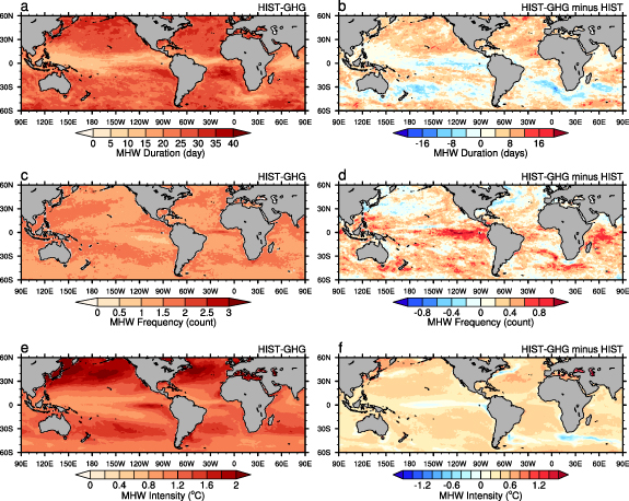
Figure 2. (a) MHW durations for the multi-model ensemble mean of the HIST-GHG simulation and (b) the difference between the HIST-GHG and HIST simulations (HIST-GHG minus HIST) averaged over 1982–2020. (c), (d) similar to (a), (b) but for annual mean MHW frequencies. (e), (f) similar to (a), (b) but for MHW intensity.
Download figure:
Standard image High-resolution imageIn comparing global MHWs in HIST-AER and HIST simulations, we find that isolated aerosol forcing significantly attenuates the intensity of MHWs on a broad scale, inhibiting their growths (figure 3). In the HIST-AER experiments, the frequency of MHWs in the eastern equatorial Pacific has markedly declined, averaging a reduction of 34% compared to historical simulations (figures 3(c) and (d)). Furthermore, there is a conspicuous decrease in MHW intensity in the mid-latitude ocean areas of the Northern Hemisphere, especially in parts of the north Pacific and the northwest Atlantic, where the intensity has fallen to one third of that in the historical simulation (figures 3(e) and (f)). This may be associated with the combined effects of climatic variabilities such as the North Atlantic Oscillation and the Pacific Decadal Oscillation (Holbrook et al 2019). The increase in anthropogenic aerosols may cause more solar radiation to be scattered back into space, reducing incident surface solar radiation, and leading to atmospheric cooling (Dittus et al 2021). This may have impacts on climate variability, including changes in SST (Wilcox et al 2015).
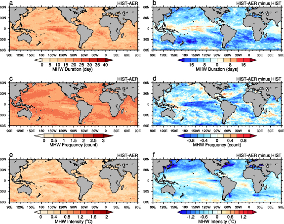
Figure 3. (a) MHW durations for the multi-model ensemble mean of the HIST-AER simulation and (b) the difference between the HIST-AER and HIST simulations (HIST-AER minus HIST) averaged over 1982–2020. (c), (d) similar to (a), (b) but for annual mean MHW frequencies. (e), (f) similar to (a), (b) but for MHW intensity.
Download figure:
Standard image High-resolution imageWe further investigate the evolution patterns of global MHWs under different climate change scenarios from 1982 to 2020. In the HIST simulation, global MHWs exhibit a significant trend of longer duration (9.93 ± 3.82 d/decade, p = 0.01), higher frequency (0.28 ± 0.17 count/decade, p = 0.01), and increased intensity (0.09 ± 0.03 °C/decade, p = 0.01, figure 4, gray line), which is consistent with results from previous studies (Oliver et al 2018, Holbrook et al 2020b). When only emissions of GHGs are considered, global MHWs show significant upward trends of duration (10.13 ± 2.78 d/decade, p = 0.01), frequency (0.06 ± 0.04 count/decade, p = 0.02), and intensity (0.18 ± 0.12 °C/decade, p = 0.01) over the past 39 years (figure 4, orange line). On the contrary, anthropogenic aerosols, if serving as the only climate forcing, would generally drive very small and insignificant declining trends of global MHW duration (−0.69 ± 0.21 d/decade, p = 0.25), frequency (−0.01 ± 0.01 count/decade, p = 0.37), and intensity (−0.01 ± 0.00 °C/decade, p = 0.33, figure 4, blue line). The uncertainties in these trends are quantified using 1 standard deviation.
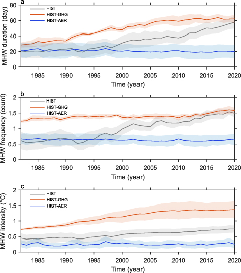
Figure 4. Time series of globally (60°S–60°N) averaged MHW (a) duration, (b) annual mean frequency and (c) intensity for the HIST (multi-model mean, dark gray; inter-model spread, light gray), HIST-GHG (multi-model mean, red; inter-model spread, light red) and HIST-AER (multi-model mean, blue; inter-model spread, light blue) simulations during 1982–2020.
Download figure:
Standard image High-resolution imageTo delve deeper into the effects of individual anthropogenic forcing agents on MHWs, we undertook a probability density function (PDF) analysis on the global mean SST anomaly. We calculate the daily SST anomaly PDFs for ten climate model single forcing experiments and historical simulation spanning from 1982 to 2020, based on their respective average climatological states, using an interval of 0.02 °C (figure 5). Our results demonstrate that anthropogenic forcings, either GHGs or aerosols, significantly alter the probability of climate extreme events, especially in the changes in the kurtosis of the PDFs. Here, kurtosis refers to the sharpness of the peak of a distribution or its 'tailedness' (the combined weight of the tails relative to the center), indicating the frequency of outliers. It is calculated as:
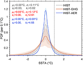
Figure 5. Globally (60°S–60°N) averaged SST anomaly (SSTA) PDFs for the HIST (multi-model mean, dark gray; inter-model spread, light gray), HIST-GHG (multi-model mean, orange; inter-model spread, light orange) and HIST-AER (multi-model mean, blue; inter-model spread, light blue) simulations during 1982–2020. For each simulation, SSTA at any location is calculated relative to the daily SST climatology over 1982–2020 at that location in that simulation. The inter-model spread is defined as one standard deviation among the 10 CMIP6 models. The 90th percentile of the PDF from the HIST simulation is denoted by gray dashed line. The PDF statistics of mean (μ, in units of oC), standard derivation (σ, in units of oC), skewness (s) and kurtosis (k) for the HIST (with the subscript H), HIST-GHG (with the subscript G), and HIST-AER (with the subscript A) simulations are shown on the top left.
Download figure:
Standard image High-resolution imagewhere x denotes SST anomaly, k,  , and
, and  denote the kurtosis, standard deviation, and mean of SST anomaly PDF, and n denotes the sampling number.
According to equation (1), the kurtosis of the PDFs in the HIST-GHG experiment decreases by 1.21 compared to the HIST simulation, extending towards both the lower and upper tails, which implies that continuous GHG emissions foster the occurrence of climate extremes such as MHWs. While in the HIST-AER experiment, the PDF curves show a noticeable increase in steepness, with the kurtosis being 1.83 higher compared to the HIST simulation. Referenced to the 90th percentile threshold of the historical simulation (gray dashed line in figure 5), this change in steepness implies aerosol effects alone inhibit climate extremes such as MHWs. Note here, according to the strong kurtosis changes, anthropogenic GHGs and aerosols can also exacerbate and mitigate cold climate extremes (i.e. the left-hand tail of distribution in figure 5) like marine cold spells (Wang et al 2022, Yao and Wang 2022, Yao et al 2022).
Based on the daily SST anomaly PDFs mentioned above, we estimate kurtosis-related warm extremes using the 99th percentile SST anomalies, which are 3.49 °C, 3.74 °C, and 2.14 °C for the HIST, HIST-GHG, and HIST-AER simulations, respectively. Therefore, for the temperatures of the warm extremes that can reach, the kurtosis differences in the HIST-GHG and HIST-AER experiments result in increases of 0.25 °C and decreases of 1.35 °C relative to the HIST simulation.
On the other hand, mean-state SST differences exist between HIST-GHG and HIST simulations, as well as between HIST-AER and HIST simulations. Relative to the HIST simulation, HIST-GHG and HIST-AER experiment show anomalous global SST warming (figure 6(a)) and cooling (figure 6(b)) from 1982 to 2020, with the exception of the North Atlantic warming/cooling hole region (Liu et al 2015, 2020, Liu and Fedorov 2019, Li et al 2023). Such mean-state global SST warming and cooling can cause PDFs to shift by 0.48 °C and −0.70 °C, respectively. Our findings suggest that the effects of kurtosis on climate extremes are comparable in magnitude to those caused by mean-state change.
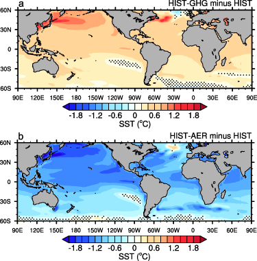
Figure 6. Climatological annual mean SST differences over 1982–2020 for the the multi-model ensembles (a) between HIST-GHG and HIST and (b) between HIST-AER and HIST. Stippling indicates where the difference is insignificant at the 95% confidence level of the Student's t-test.
Download figure:
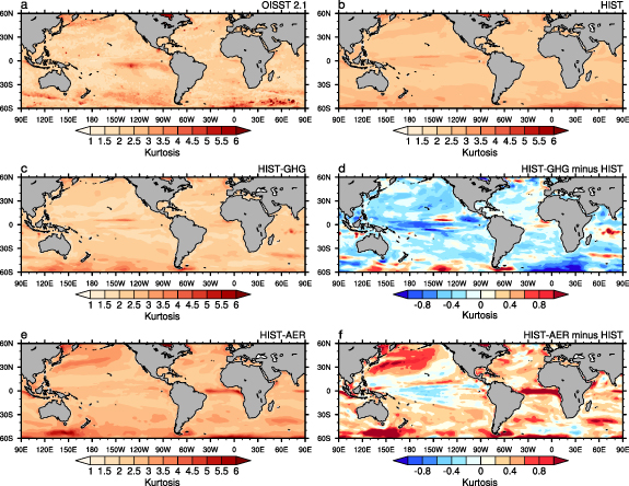
Standard image High-resolution imageAdditionally, we look at the global pattern of kurtosis inferred from daily SST anomaly PDF at each location over the period 1982–2020 for observation and model simulations. We find that the HIST simulation can typically well capture the observed feature of large kurtosis in the central and eastern equatorial Pacific as well as over oceans poleward than 30°N and 30°S (figures 7(a) and (b)). Compared to the HIST simulation, the HIST-GHG (figures 7(c) and (d)) and HIST-AER experiments (figures 7(e) and (f)) show smaller and larger kurtosis generally over a global scale, respectively, which is consistent with the patterns of MHW difference discussed previously (figures 2(b), (d), (f) and 4(b), (d), (f)).
Figure 7. SSTA PDF kurtosis of (a) OISST v2.1 and the multi-model ensemble means of the (b) HIST, (c) HIST-GHG, and (e) HIST-AER simulations averaged over 1982–2020. Panels (d) and (f) shows the kurtosis differences (d) between HIST-GHG and HIST and (f) between HIST-AER and HIST.
Download figure:
Standard image High-resolution image
4. Discussions and conclusions
In this study, we identify the distinct roles of anthropogenic GHGs and aerosols on the frequency, intensity, and duration of global MHW during the past 39 years based on CMIP6 historical simulation and associated single forcing experiments. We find that anthropogenic GHGs and aerosols can modulate the shape of SST probability distribution and hence the statistics of MHWs. When only alterations in GHGs are considered, the PDF of SST anomaly shows smaller kurtosis and more extended tails than the HIST simulation. Correspondingly, MHWs display longer duration, larger frequency, and intensity over a global scale. On the other hand, under the scenario that is driven only by human-induced aerosols, the PDF of SST anomaly shows large kurtosis and less extended tails than the real-world case, and accordingly, global MHWs commonly happen less frequently with smaller intensity and shorter durations over the past 39 years. We also discover that the magnitude of kurtosis's effects on climate extremes is comparable to that of mean-state change.
Our study highlights the profound effects of anthropogenic GHGs and aerosols on global MHWs, which are far beyond the perception that they simply act to shift the SST probability distribution by modifying mean-state SST as a consequence of GHG warming and aerosol cooling. Our results are critically important for predicting future MHW events and formulating effective strategies for marine resource management and climate adaptation. However, since daily outputs of surface heat flux, ocean advection and diffusion are not available in the CMIP6 archives, we are unable to conduct oceanic mixed-layer heat budget analysis on a daily scale to elucidate the physical mechanisms for GHG- and aerosol-driven MHWs. We will leave this for future studies. Furthermore, many other human-induced climate change factors, such as stratospheric ozone depletion and tropospheric ozone increase (Liu et al 2022), could influence the characteristics of global MHW. These also require further consideration in future research.
Acknowledgments
This work is supported by grants to W L from U.S. NSF (AGS-2053121, OCE-2123422 and AGS-2237743). W L and R J A are supported by U.S. NSF AGS-2153486. W L is also supported by the Hellman Fellows Fund as a Hellman Fellow.
Data availability statement
OISST v2.1 data are publicly available at: https://www.ncei.noaa.gov/products/optimum-interpolation-sst.
The data that support the findings of this study are openly available at the following URL/DOI: https://esgf-node.llnl.gov/search/cmip6/.
Conflict of interest
The authors declare no competing financial interests.