

Abstract
In the Mediterranean basin, climate change signals are often representative of atmospheric transients in precipitation patterns. Remote mountaintop rainfall stations are far from human influence and can more easily unveil climate signals to improve the accuracy of long-term forecasts. In this study, the world's longest annual precipitation time-series (1884–2021) from a remote station, the Montevergine site (1284 m a.s.l.) in southern Italy, was investigated to explain its forecast performance in the coming decades, offering a representative case study for the central Mediterranean. For this purpose, a Seasonal AutoRegressive-exogenous Time Varying process with Exponential Generalised Autoregressive Conditional Heteroscedasticity (SARX(TVAR)-EGARCH) model was developed for the training period 1884–1991, validated for the interval 1992–2021, and used to make forecasts for the time-horizon 2022–2051, with the support of an exogenous variable (dipole mode index). Throughout this forecast period, the dominant feature is the emergence of an incipient and strong upward drought trend in precipitation until 2035. After this change-point, rainfall increases again, more slightly, but with considerable values towards the end of the forecast period. Although uncertainties remain, the results are promising and encourage the use of SARX(TVAR)-EGARCH in climate studies and forecasts in mountain sites.
Export citation and abstract BibTeX RIS

Original content from this work may be used under the terms of the Creative Commons Attribution 4.0 license. Any further distribution of this work must maintain attribution to the author(s) and the title of the work, journal citation and DOI.
1. Introduction
Our knowledge and understanding of the climatic characteristics of mountainous regions is limited both by the paucity of observations (Yokohata et al 2021) and by the limited attention paid to the effect of spatial scales on weather and climate, and their complex interactions (Barry 1994, Goldenson et al 2018). At the same time, remote mountaintop precipitation stations are less influenced by anthropogenic activities and can more easily reveal climate signals, enhancing the reliability of long-term forecasts. There is also a growing need for precipitation forecasting due to the important role of rainfall and relative control over the water cycle in water resources management (Diodato et al 2017), and global groundwater storage (Li et al 2019).
Climate predictions are widely used in climate change studies (Arnell and Delaney 2006, Xu et al 2009). Although global circulation models (GCMs) have been developed and refined over the years for climate projections, these are large-scale models that are not area-specific. Local precipitation tends to be better estimated with high-resolution regional climate model (RCMs), largely due to better resolved orography (Schiemann et al 2020), but even RCM projections that rely on an ensemble of climate models are not always able to improve on GCM-driven simulation skills (Fereday et al 2018, Dosio et al 2019). These projections offer a range of 'plausible' descriptions of how the future climate may evolve (van Vuuren et al 2011). However, errors exceeding 100% in precipitation estimates are frequently observed in state-of-the-art climate models, as highlighted by Tapiador et al (2019). This illustrates the considerable difficulties involved in accurately predicting this complex variable. Unlike temperature projection uncertainty, which is primarily driven by the unpredictability of future anthropogenic greenhouse gas emissions and their resulting atmospheric concentrations (accounting for 61% of uncertainty in Coupled Model Intercomparison Project Phase 6), the contribution of emission scenario uncertainty to precipitation projections is relatively low, at approximately 1.8% (Wu et al 2022). This indicates that the primary challenge in accurately estimating future precipitation patterns lies in the modelling process itself. Also, currently operational drought forecasts in Europe focus on day-to-month outlooks (e.g. Cassou 2008), such as the short-term drought severity indicator and the monthly rainfall outlook generated by the ensemble prediction system for medium-range and extended forecasts of the European Centre for Medium-Range Weather Forecasts (www.ecmwf.int). These forecasts are overly constrained by short-duration weather phenomena (Chikamoto et al 2020), as unpredictable atmospheric noise makes interannual to decadal climate prediction challenging (Smith et al 2019). Conversely, Leith (1975) used the fluctuation-dissipation theorem of statistical mechanics to show that the use of a complex model does not always predict future conditions better than using a simpler statistical model. From a statistical point of view (e.g. Dimri et al 2020), the dynamic structure of climate is driven by local changes in precipitation and temperature, and studies focusing on the assessment of climatic change are often based on the analysis of temperature and precipitation time-series using the approach known as time series analysis (TSA). However, here too, accurate forecasts are difficult to make, especially for many hydrological time-series given their non-stationarity and chaos (Wang et al 2018). In general, this is because time-series are often affected by different hidden patterns that may appear as trends, cycles and variations around a mean, or irregular variations.
Already in historical times, climate was the subject of calculations to account for these patterns. Thus, the English philosopher and statesman Francis Bacon (1561–1626) wrote in Essay LVIII, 3rd/final edition of 1625 (Hardy et al 1983, p 147):
There is a strange idea that I have heard and I would not say that it is to throw away without thinking about it over a little. They say it is observed that every thirty-five years the same type and kind of weather appears again, as great frosts, great storm, great droughts ... it is something I mention, because running calculations backwards, I found some coincidence.
Today, evolving statistical approaches have made it possible to model these patterns and TSA tools have become suitable approaches for assessment and forecasting, in particular in cases where precipitation variability was guaranteed to be reflected in the evolution of highly predictable chaotic dynamics. Efforts to use time-series autoregressive moving average (ARIMA) models to forecast hydrological data are intensifying. In particular, seasonal ARIMA (SARIMA) models have been successful in short-term rainfall forecasts (Eni and Adeyeye 2015). The exceptional accuracy of ARIMA models in predicting monthly rainfall has justified the study by Swain et al (2018), who forecasted over a long-time period of 20 years. On the other hand, Unnikrishnan and Jothiprakash (2020) proposed the integration of singular spectrum analysis, ARIMA and artificial neural networks (ANNs) in a hybrid model to predict daily rainfall in a catchment with reliable accuracy. At the same time, decadal forecasting of hydrological data is in its early stages due to lack of knowledge of hydrological predictability and forecasting skill at interannual to decadal scales (Zhu et al 2019), particularly in Italy, where little has been published (Diodato et al 2017, Zirulia et al 2021). However, with the lack of knowledge of complex atmospheric processes, the uncertainty of forecasts increases with the lead time (Diodato et al 2019, Ashok and Pekkat 2022).
Here we address the issue of the reliability of long-term forecasting using the ARIMA model and the Exponential Generalised Autoregressive Conditional Heteroscedasticity (EGARCH) technique for understanding climate trend variability and for water resource management in the Mediterranean region, which has been identified as a hotspot for climate change and where sub-regional studies are recommended (Hartmann et al 2013, Romano et al 2022). In this context, the climate signals detected in the remote site of Montevergine (southern Italy) are particularly representative of the climate change associated with the rainy transient across the Mediterranean. However, issues related to the lack of ancillary information and observation may prevent statistical analyses in precipitation forecasting (after Horner et al 2019). Thus, we took the opportunity to use the annual precipitation records at Montevergine for 138 years (1884–2021), to investigate the importance of time-series memory for any influence on the point forecast for 30 years ahead (i.e. 2022–2051). Specifically, a Seasonal AutoRegressive Time-Varying process with exogenous variables [SARX(TVAR)] was coupled to the EGARCH technique with the incorporation of an ancillary variable (dipole mode index, DMI) to mitigate missing information in the forecast period. We assessed the ability of the SARX(TVAR)-EGARCH approach to display a predictable temporal pattern, resolving and overcoming the difficulties affecting physically-based models and paving the way for the use of data-driven algorithms and TSA models in precipitation forecast. The autoregressive-exogenous (SARX) model, which assumes that the current system output is a function of both previous system outputs and inputs was compared to the pure autoregressive SAR model (without exogenous variable), which assumes that current system output is only a function of the previous system outputs.
2. Environmental setting and model building
2.1. Study site
The Montevergine massif (also known as Partenio) is part of the Campanian sub-Apennine, located in southern Italy (figures 1(a) and (b)) in an eccentric position with respect to the ridge chain that divides the Italian peninsula into Adriatic and Tyrrhenian parts (figures 1(b) and (c)). The Montevergine Observatory is located at 40° 56ʹ North and 14° 43ʹ East, at 1270 m a.s.l., overlooking the Sabato Valley (figure 1(c)). From the top of the observatory, the view extends south-eastwards for more than 100 km to the regions Molise, Apulia (east) and Basilicata (south). The Montevergine Observatory is located in the free troposphere, far from anthropogenic influence. The data used in this study were provided by Father Amato Gubitosa, observatory's director from 1968 to 2006, extracted from the original registers and then screened, with the additional support of the metadata recorded in the Observatory's chronicles. After 2006, the Observatory was renovated and provided with new equipment, including digital instruments, thanks to the new director, Father Benedetto Komar (observatory's director from 2007). The update after this date is taken from Capozzi and Budillon (2013), and from the Montevergine Observatory website (www.mvobsv.org), as provided annually.
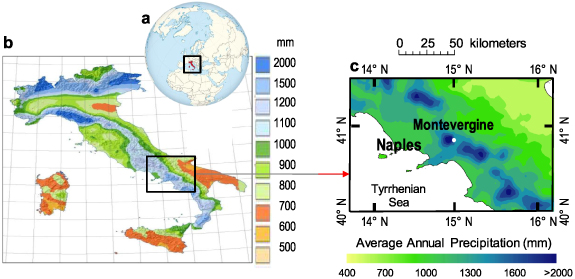
Figure 1. Geographic setting of the study site. (a) Central Mediterranean area (black square). Reproduced from Wikipedia. CC BY-SA 3.0. This Italy on the globe (Europe centred) image has been obtained by the author(s) from the Wikipedia website where it was made available under a CC BY-SA 3.0 licence. It is included within this article on that basis. It is attributed to TUBS. (b) Mean annual precipitation in Italy during 1996–2015. Reproduced from ISPRA. CC BY 4.0. (c) Downscaling of mean annual precipitation in the Campania region during 1971–2010 (by ordinary cokriging via ArcGIS Geostatistical Analyst—Environmental Systems Research Institute—on the SCIA database. Data reproduced from SCIA database).
Download figure:
Standard image High-resolution image2.2. Climatic and seasonal patterns
The Montevergine Observatory (1284 m a.s.l.) clings to the deposits of the homonymous mountain (figure 2(a)) and the eastern head of Mount Partenio (figure 2(b)). According to the Köppen–Geiger classification (Beck et al 2018), the observatory lies within zone Cs (Mediterranean climate), where the effects of elevation on temperature introduce climatic gradients starting in the low-lying surroundings, characterised by a high mean annual temperature (Lanfredi et al 2015), and ending in the cooler, higher elevations. In particular, the observatory is characterised by warm-summer climate (Köppen code Csb). The climate in these Mediterranean areas exhibits a large seasonal contrast and seasonal precipitation displays evident minima in summer (e.g. Lanfredi et al 2020), which is also the warmest period.
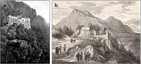
Figure 2. Montevergine Abbey. (a) View of the east side. Adapted with permission from (Leah 1852). (b) Montevergine Mountain, xylography. Reproduced with permission from (Gourdault 1877). Image kindly granted by www.lapuntaseccastampeantiche.com.
Download figure:
Standard image High-resolution imageThe phenomena responsible for the activity of precipitation systems in the Montevergine area and its surroundings are determined by the convergence of humid air masses towards different cyclonic situations attributable to the encounter of air masses with differential thermal characteristics in the central Mediterranean basin. In fact, the climate of this central part of the Mediterranean is part of the complex of interactions between cold air masses from northern Europe and tropical air masses, which are at the origin of the so-called Mediterranean cyclogenesis (Buzzi and Tosi 1991). These lows have the greatest impact in northern Italy and along the Tyrrhenian peninsular coast, where rainfall variability is most prominent (figure 1(b)). If we perform a spatial visualization around the study area, we can appreciate in more detail the variability of the precipitation field along the Campania region and surrounding Montevergine (figure 1(c)).
These differences are likely due to the different altitudes and geographical positions of the locations, as well as to the different directions of the moist air flows, which can lead to an intensification of the water vapour condensation process when precipitation systems are forced to overcome the sub-Apennine chain and release more rain that moves eastwards into the basin hinterland.
2.3. Explanatory data analysis
The exploratory analysis of the data can start with the visualisation of the precipitation time-series. A time-series is a chronologically ordered set of observations made at regular intervals over a given period of time (which in our case is annual). Forecasting methods using time-series assume that future values can be extrapolated from past values. To discover the underlying behaviour of the time-series, a preliminary visual examination of the data is necessary. This is usually done by analysing statistical data and plotting cycles. Trends, cycles and variations around a mean are possible patterns. There may also be irregular or random variations. In addition, to establish stationarity, it is necessary to examine the variation in the mean and variance, and the heteroscedasticity of the data, respectively.
The evolution of the Montevergine precipitation time-series from 1884 to 2021 can be used to start an exploratory analysis of the data (figure 3). The evolution of the annual precipitation is shown in figure 3(a), and the downward trend is significantly supported (p < 0.01) by the Mann–Kendall test (figure 3(a), linear trend in black bold). Furthermore, the histogram is far from a Gaussian distribution (figure 3(b)), and the quantiles are not normally distributed (p < 0.01) in the QQ-plot (figure 3(c)).

Figure 3. Montevergine precipitation data (1884–2021). (a) Annual time-series and its regression line; (b) its histogram; (c) its QQ-plot; (d) variance estimates with an 11 year moving window and its regression line; (e) its histogram; (f) its QQ-plot.
Download figure:
Standard image High-resolution imageThe evolution of the variance also shows a significant decreasing (p < 0.05) Mann–Kendall trend (figure 3(d), linear trend in black bold), while also in this case the histogram pattern (figure 3(e)) and the QQ-plot (dotted line in figure 3(f)) deviate from a normal distribution (blue line). In summary, the precipitation time-series appears to be non-stationary in first and second order. This should steer our research toward models in which variance and autocorrelation do not remain constant over time, and in which heteroscedasticity is taken into account at the same time.
2.4. Time-series memory and predictability
The exploratory analysis of the data can be taken further by estimating the Hurst (H) exponent and performing a dynamic analysis in the space-time domain.
The rate of stochastic processes in a time-series is defined by the exponent 0 ⩽ H ⩽ 1, which is related to the fractal dimension D of the time-series by the relation D = 2 − H and provides a measure of its autocorrelation (long-term memory) qualities. When the time-series is persistent or trending, the exponent H is >0.5 (random walk), which implies a long memory effects. On the other hand, when H < 0.5 we have an anti-persistent time-series signal, which means that whenever the time-series went up in the last period, it is more likely to go down in the next period (more irregular than a pure random walk with H = 0.5). Using the SELFIS self-similarity analysis software (www.cs.ucr.edu/tkarag/Selfis/Selfis.html), we estimated the variance ratio of the residuals on the detrended time-series, which is known to be an unbiased estimator of H in almost all its ranges (Sheng and Chen 2009). To do this, we first used the source time-series to estimate the exponent H, determine whether there is a long memory effect, what type of it, and whether this memory can be echoed into the future, in the forecasting phase. In the Montevergine case, this gives an exponent H of 0.66 (figure 4(a)).
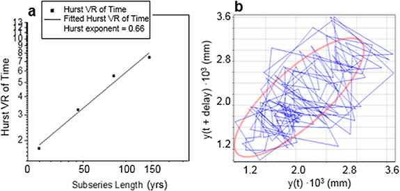
Figure 4. Montevergine precipitation Hurst exponent (1884–2021). (a) Detrended residual variance ratio (VR) method estimate; (b) time-series attractor in the phase-space domain (blue trajectory) with ellipse-like branching (red contour).
Download figure:
Standard image High-resolution imageThis indicates that the effect exists and is positive, i.e. if the time-series has increased in the past, it will continue to do so in the future, and vice versa; and since H > 0.65, the exponent suggests that the memory can be used to propagate into the future. While H is important in determining the memory strength of the time-series and its susceptibility to forecasting, it does not provide us with any information about the reliability of the forecast.
The space-time attractor helps us to do this. After a sufficiently long time, the attractor is a set towards which an initially perturbed dynamic system evolves. If the system evolves in an orderly fashion after the perturbation, the forecast is reliable: if not, it is not. Next, the reliability properties of the precipitation time-series forecast, a crucial step in non-linear TSA, were determined. In the time-state domain, it is observed that the precipitation attractors (towards which the system tends to evolve) remain more entangled around a directional branching (figure 4(b), red ellipse), indicating a potentially predictable pattern (if reasonably accurate forecasts can be made).
2.5. Model start selection criteria
Figure 5 shows the estimated autocorrelation function (ACF) between precipitation values at various lags over the residual values. The lag k measures the correlation between the standardised residuals of precipitation at time t and time t + k after taking into account all lower lags. It can be used to determine the order of the autoregressive model needed to fit the data. There are also 95% confidence limits around 0. At the 95% confidence level, there is a statistically significant correlation in that lag if the probability limits of that lag do not contain the estimated coefficient. Since the ACF (figure 5(a)) and the partial ACF (PACF, figure 5(b)) also describe the shape of the exponentially decreasing autocorrelation of the residuals, and with the ACF having the first two spikes at lags 1 and 2, and the PACF having a single spike at lag 1. According to Valenzuela et al (2008), this ACF can be used to determine the order of the autoregressive model needed to fit the data, indicating that the time-series is generated, to a first approximation, by an AR(2,0,0) process.
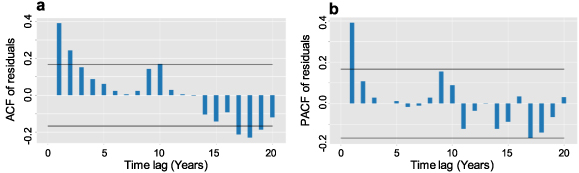
Figure 5. Standardised Montevergine precipitation residuals (1884–2021). (a) Autocorrelation function (ACF); (b) partial autocorrelation function (PACF). The horizontal black lines indicate the 95% confidence level limits.
Download figure:
Standard image High-resolution image2.6. Model-building process
Models can bring together the work of multiple research teams into single operational outputs that can summarise knowledge as effectively, if not better, than traditional scientific outputs (Mulligan and Wainwright 2004). Simulation models can also incorporate the effects of simple processes on complex spaces, as well as the accumulation of the effects of those same processes and their variations over time (Mulligan and Wainwright 2004). However, the greatest benefits of implementing the models are seen when they are used for forecasting. As far as we know, precipitation dynamics based on the periodicity of rainfall, the lag time, represents the maximum amount of information that can be borrowed between the states at time t − 1 and time t. However, since the variability of our precipitation time-series, as well as the non-stationarity of its variance, results in chaotic dynamics with high predictability, the integration of a seasonal model with time-varying parameters will be appropriate.
As it was found in section 2.5 that variance and autocorrelation are not constant over time, the autoregressive model was modified to account for seasonality (m) and time-varying processes. As a result, figure 6 illustrates a schematic procedure for forecasting future precipitation, where the technological framework presents the main steps of the SARX(TVAR)-EGARCH modelling, which was chosen for this case study.
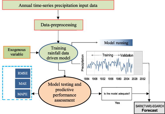
Figure 6. Schematic workflow of the SARX(TVAR)-EGARCH model forecasting procedure.
Download figure:
Standard image High-resolution imageIn a first step, it is assumed that the random variable y at time t (yt
), not only depends on  , but fluctuates with a constant period m. Thus, one way to also represent the seasonal (periodic) member in the seasonal autoregressive model is by means of an additive component, where the process is assumed to be essentially composed of two parts.
The first is regarded as a location component (Montgomery et al 2008):

where St is the stochastic part, which can be modelled as an AR (autoregressive) process plus a mt (deterministic) member with seasonal length (period) m. In this sense, yt can be viewed as a process with predictable periodic behaviour with some elements above (Montgomery et al 2008). In particular, to account for autocorrelation, we developed the stochastic and deterministic components in the form of a seasonal autoregressive model of order [p, d, q] × [P, D, Q]m (where p = 2 is the number of autoregressive terms, d = 0 is the number of non-seasonal differences, and q = 0 is the number of lagged forecast errors in the prediction equation, while P= 2, D= 0 and Q= 0 are their corresponding seasonal parameters), with a time-varying process model (Basawa et al 2004):
where  is the time-series of precipitation to be forecasted at time t over the year with period m; the first term is the stochastic member, while the second is the deterministic-seasonal term, and the third member (coupled sum) is the seasonal adjusted component; X is the exogenous variable; ω is the white noise with an uncorrelated process of zero mean and constant variance σ2; φ is the autoregressive parameter, while κj
is the term associated with the seasonal component. The letter L represents the location component in equation (2), while S represents the log-scale component in equation (3).
is the time-series of precipitation to be forecasted at time t over the year with period m; the first term is the stochastic member, while the second is the deterministic-seasonal term, and the third member (coupled sum) is the seasonal adjusted component; X is the exogenous variable; ω is the white noise with an uncorrelated process of zero mean and constant variance σ2; φ is the autoregressive parameter, while κj
is the term associated with the seasonal component. The letter L represents the location component in equation (2), while S represents the log-scale component in equation (3).
The second component is logarithmic and takes into account heteroscedasticity:

where φ(S)i, κ(S)j and ω(S) are the EGARCH parameters, while σ is the standard deviation, and γ accounts for the leverage effect (de la Fuente et al 2020). The SARX(TVAR)[p,0,0] × [P,0,0]m parameters in equation (2), and EGARCH (P,0,Q)ms in equation (3) (where ms= 3 is the periodic cycle associated with the log-scale component), were selected from the ACF and validation test. As for the variance equation, we find a symmetric effect, φi (S), significantly different from zero, while, as the conditional volatility is not very persistent, κ(S)j is small and significantly not different from zero. Further insights and numerical solutions of equation (2) can be found in Basawa et al (2004) and Lit et al (2019–2023). Forecasts were performed with the Time Series Lab, Dynamics Edition software (https://timeserieslab.com), and the Visual Recurrence Analysis (https://visual-recurrence-analysis.software.informer.com/4.9).
3. Results and discussion
3.1. Influence of the exogenous variable
The inclusion of exogenous variables in forecasting models requires caution, as advised in the literature (Chatfield 2000). Petropoulos et al (2022) discussed the challenges and limitations associated with incorporating exogenous variables, emphasising the risks of spurious correlations and increased model complexity when multiple variables are included. In this study, We employed the Seasonal AutoRegressive-eXogenous Time Varying process [SAR(TVAR)] with EGARCH to extract and quantify the direct influence of an exogenous variable on annual precipitation. For this purpose, we adopted an index that represents key climate variability in the Mediterranean: the DMI. Orbital changes affect the Indian Ocean dipole's sea surface temperature pattern, with induced changes in regional seasonality (Brierley et al 2023). In particular, a dominant mode of the interannual variability of Indian summer monsoon rainfall shows a west–east dipole pattern, which is linked to the active Azores High (Yadav 2021).
The active Azores High is associated with enhanced subsidence, which results in massive convergence in the upper troposphere. This creates a meridional vorticity dipole composed of an anomalous cyclonic and anti-cyclonic circulation at 30° N and 50° N, respectively, and enhances the Rossby wave source (RWS). RWS is one of the mechanisms responsible for teleconnections (Qin and Robinson 1993), as Rossby waves appearing in the atmosphere as a result of vertical motion and upper‐tropospheric divergence cause anomalous upper-level vorticity and, in turn, this vorticity induces the formation of wave trains (Sardeshmukh and Hoskins 1988). The Rossby wave train cascades down, imposing successive anomalous negative geopotential heights over the northern Mediterranean (Yadav 2021). Figure 7(a) shows the linear correlation between this index (DMI) and annual precipitation at Montevergine Observatory. It follows that few data points fall within the 95% prediction limits, and only five points outside this limit. Since the p-value in the ANOVA is less than 0.05, we can conclude that there is a statistically significant relationship between precipitation and filtered DMI at 95% confidence level (Pearson's correlation coefficient equal to 0.51), which means that the DMI was suitable to support the Montevergine precipitation forecast. In this way, the DMI time-series was validated for the period 1992-2021 (Appendix
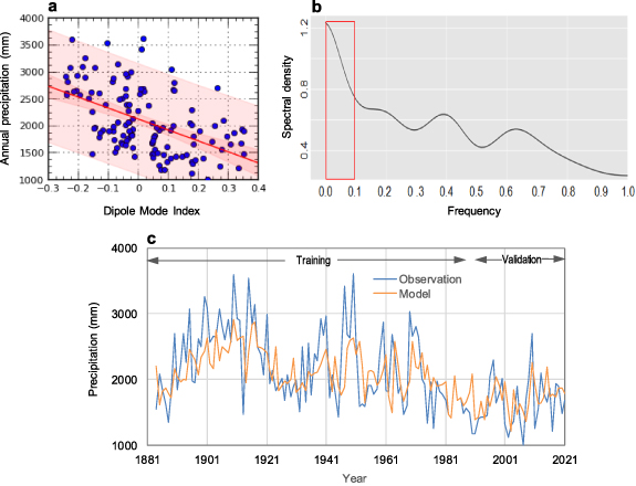
Figure 7. Application of the model in forecasting precipitation with an exogenous variable. (a) Scatterplot between annual precipitation at Montevergine over the period 1884–2021 and the dipole mode index, with the inner (deep pink area) and outer (light pink area) bounds indicating the 90% and 95% confidence limits, respectively; (b) spectral frequency density of Montevergine precipitation time-series, with the likely window (red box) where the SARX(TVAR)-EGARCH model cycle is located; (c) modelled (orange line) and observed (blue line) annual precipitation data (mm) for the Montevergine time-series.
Download figure:
Standard image High-resolution image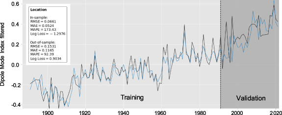
Figure 2A. Annual filtered (11-year moving window + 0.5 × DMIt), modelled (blue line) and observed (black line) dipole mode index data over the period 1880–2021.
Download figure:
Standard image High-resolution image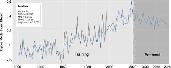
Figure 3A. Time evolution of the filtered annual data of the observed dipole mode index annual filtered data (11-year moving window + 0.5 × DMIt), in 1920–2021 (black line) and forecasted in 2022–2051 years (blue line).
Download figure:
Standard image High-resolution image3.2. Candidate model
The autoregressive component is non-stationary in the SARX(TVAR)-EGARCH model, while the sum of the m seasonal components must be equal to zero. This is fulfilled by estimating the first m− 1 components, which together with the zero-sum limit determines the last component (Lit et al 2019–2023). The frequency spectrum is a chart that provides information on the amplitude of the cyclic components for a given frequency range, as well as the length of m.
The predicted frequency spectrum for the current SARX(TVAR)-EGARCH seasonal model parameters fitted to the precipitation data is shown in figure 7(b), with the predominant cycles between 1/f(0.01) and 1/f(0.1) (figure 7(b), red box), as successive frequencies have descending spectral values. In this way, operating in the high cycle window, and with validation support (after several trials), the cycle was set to 1/f(0.029), corresponding to a period m equal to ≈20 years. This agrees well with the pattern we observe in the time-series plot in figure 7(c). Thus, the best candidate model for our data is a time-varying process approach is expressed by a SARX(TVAR)[AR(2,1) + Periodical (m= 20) + X β + Score(1)] model plus an EGARCH[exp(AR(2,1) + Periodical (ms = 3) + Leverage + Score(1))] model.
3.3. Parameterisation and evaluation of SARX(TVAR)-EGARCH model
Figure 7(c) shows the co-evolution between the model and the observed data during the training (1884–1991) and validation (1992–2021) periods with the SARX(TVAR)[2,0,0] × [2,0,0]20 − EGARCH[2,0,1]3 model.
The consistency between the two respective lines (orange and blue) shows that the coupled pattern in the validation period is similar to that of the training epoch. The error statistics of the training and validation periods are presented in table 1. The 30 data values at the end of the time-series were then used to calculate model validation error statistics. The forecast errors need to be checked to ensure that the forecast is working correctly. The first three statistics are used to calculate the magnitude of the errors. Since the results of the validation period (1992–2021) are comparable to those of the training period (1884–1991, table 1), it is likely that the model will perform as well as expected in the future projection. The Log Loss function (with values of 7–8) serves a metric of uncertainty, and there is no agreed-upon threshold for determining an acceptable Log Loss value. However, a mean absolute percentage error (MAPE) of about 20% stands out, as it suggests an acceptable level of accuracy (<25%, Swanson et al 2011) for forecasts that aim to capture long-term trends and patterns of precipitation. Additionally, the Kling–Gupta efficiency index, ranging from −∞ to 1, exceeding −0.41 (Knoben et al 2019) indicates that the model outperforms the benchmark predictor represented by the mean of observations with limited uncertainty in the model's estimates.
Table 1. SAR(TVAR)-EGARCH model performance for the training (1884–1991) and validation (1992–2021) periods for the Montevergine precipitation time-series. RMSE: root mean square error (optimum, 0 to +∞, worst); MAE: mean absolute error (optimum, 0 to +∞, worst); MAPE: mean absolute percentage error (optimum, 0 to +∞, worst); Log Loss: logarithmic loss (optimum, 0 to +∞, worst); KGE: Kling–Gupta efficiency index (worst, −∞ to 1, optimum).
| SARX(TVA)-EGARCH model | ||
|---|---|---|
| Statistics | Training period (1884–1992) | Validation period (1993–2021) |
| RMSE (mm) | 487 | 370 |
| MAE (mm) | 375 | 317 |
| MAPE (%) | 17 | 21 |
| Log Loss | 7.40 | 7.61 |
| KGE | 0.50 | 0.48 |
Instead, the SARX(TVAR)-EGARCH parameterisation for model forecasting was performed over the entire 1884–2021 (138 years) precipitation time-series, so that the most recent part of the time-series is accessible as helpful information for future forecasting. In Appendix

Figure 1B. SARX(TVAR)-EGARCH model parameters in the training forecast of equation (2) for Montevergine precipitation to location and scale components.
Download figure:
Standard image High-resolution image3.4. Normality diagnostic checks
We can now examine the normality tests in more detail after using the SARX(TVAR)-EGARCH model, which shows that the residuals are approximatively free of heteroscedasticity. The quality of any model should be determined by examining whether the residuals form a white noise process through a series of goodness-of-fit tests (Jere and Moyo 2016).
The histogram in figure 8(a) shows that the mean residual is around 0 and the pattern of residuals reflects a Gaussian shape. QQ plots are a useful tool for determining normality. The QQ plot of the residuals in figure 8(b) shows that the points (empty black dots) follow the blue straight line within the confidence interval (blue dashed line), indicating that the residuals have a normal distribution.

Figure 8. Residuals of the SARX(TVAR)-EGARCH model (1884–2021). (a) Histogram and fitted normal density; (b) QQ-plot (dots) with confidence interval (blue dashed lines) of residuals.
Download figure:
Standard image High-resolution image3.5. Annual precipitation forecast
Montevergine precipitation is representative of atmospheric transients in the central Mediterranean and thus suggests that its oscillations can be considered large-scale phenomena. This determines a climatic signal and its possible evolution and variability changing along the branching process of future precipitation dictated by the current forecasting approach.
Graphical inspection of the annual precipitation forecasts in figure 9(a) reveals that the extremes of the future precipitation trend are expected to remain within the range of maximum variability of the past 30 years. However, the zoom in the precipitation forecast trajectory (figure 9(b), black line) lies roughly in the range between −1 and +2 standard deviation, between 2022 and 2051. The range defined by twice the standard deviation offers an estimate of the expected variability in the forecasts, indicating that the model is effectively capturing the inherent uncertainty in the forecasted data. The presence of variability around the long-term mean suggests that the model is not excessively biased and is capable of generating predictions that are not constant over time. Specifically, at the beginning of this period, the forecast values are just below the mean. Subsequently, there are two notable jumps (beyond twice the standard deviations) in growth between the intervals 2022–2035 and 2036–2051. These variations indicate that the model is able to capture shifts and changes in the underlying patterns, allowing for dynamic forecasts that reflect the evolving nature of the data.
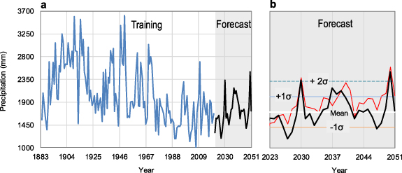
Figure 9. Time evolution of annual precipitation. (a) Measured (1884–2021; blue line) and forecasted (2022–2051; black line) data; (b) relative zoom on the forecast period (2022–2051) in which the long-term mean value (white line) and ±1σ (blue and orange lines), and +2σ (dashed blue line) are indicated. Red line represents the pure SAR(TVAR)-EGARCH, that is the model without the auxiliary variable (dipole mode index).
Download figure:
Standard image High-resolution imageThus, the dominant feature for the whole forecast period is a significant upward trend (Mann–Kendall p < 0.05), with a gradual departure from the past and current drought regime, up to the change-point in 2035 (Mann–Whitney–Pettitt test; Pettitt 1979), which was examined over the period 1991–2051 to include a 60 year period starting 30 years before the end of the observations. Thereafter, an atmospheric transient in the central Mediterranean could establish an above-average rainfall regime.
This is in line with the prospected forthcoming terrestrial cooling (Zharkova et al 2015, Zharkova 2020), which would lead to increased rainfall in Italy (Conte et al 1991), if also Europe and the central Mediterranean were to be affected by the temperature decrease, as stated in Omrani et al (2022). Winter Atlantic Multidecadal variability in the period 2020–2050 can be considered as an additional positive feedback for increased precipitation over the Mediterranean. The cold season of a Mediterranean sub-region requires two to four patterns to explain 33%–54% of the precipitation variability and five to eight patterns to explain 56%–78% (Norrant 2004).
Time-series of precipitation anomalies (relative to 1986–2005 mean) indicate much higher interannual variability for the southern part of the Mediterranean, which is evident in both historical simulations and future scenarios (Zittis et al 2019). Moreover, climate models suggest a decrease in precipitation down to −60% for RCP8.5 (the most extreme global greenhouse gas emission pathway) by the end of the 21st century. On average, the moderate RCP2.6 scenario indicates much less drying (−5%–10% decrease in precipitation) in the southern Mediterranean, while a small increase in precipitation (related to the northward migration of storm tracks) is suggested. However, again the signal is much weaker than natural interannual variability (Zittis et al 2019). The latter depends on both dynamical and thermodynamic processes, which Raible et al (2018, 2020) argue may be equally important in cyclone-induced precipitation fluctuations. This contrasts with future climate projection studies that show a large increase in cyclone-related precipitation extremes (e.g. Zappa et al 2013, Pfahl and Sprenger 2016, Yettella and Kay 2017, Zhang and Colle 2017, Hawcroft et al 2018). The main processes underlying this increase are based on thermodynamics, according to which a warmer atmosphere can hold more moisture (based on the Clausius–Clapeyron relation that the water-holding capacity of the atmosphere increases by about 7% for every 1 °C increase in temperature), so more intense precipitation extremes are expected under warmer conditions (O'Gorman and Schneider 2009, Berg et al 2013). These studies emphasise the Mediterranean region's high sensitivity to climate variability and the impacts of global climate change. The comparison between the pure SAR(TVAR)-EGARCH model (figure 9(b), red line) and the established SARX(TVAR)-EGARCH model (without the DMI auxiliary variable) revealed that the former outperformed the latter, displaying agreement in both overall and cyclical trends. Consequently, these findings enhance the reliability of the predictions presented in this study. Notably, the incorporation of climate variables such as the DMI into predictive models can improve the accuracy of predictions for particularly sensitive areas (e.g. Kusumastuty et al 2021) and instils greater confidence in addressing the challenges posed by climate change.
4. Concluding remarks
4.1. Advancing decadal precipitation forecast
The study of decadal-scale projections is an evolving field that relies on intermediate complexity models. In contrast, statistical modelling in meteorology and climatology has made only modest progress, particularly regarding the hydrology of small Mediterranean catchments and sites in response to climate change. In an effort to address this gap, we have developed a statistical forecast approach that aims to anchor the precipitation reality (annual time-series) to past observed changes and replicate these changes in the near future (over a three-decade period). In particular, this work presents a data-driven seasonal (periodic) autoregressive statistical approach to create 30 year (2022–2051) precipitation forecasts specific to the remote Montevergine site from local historical measurements (1884–2021). The SARX(TVAR)-EGARCH model was created using the log-likelihood criterion and validated from 1992 to 2021. The selected forecast period of 30 years, which aligns with the validation period of 30 years, is deemed reliable for capturing interannual variations beyond individual annual figures. To minimise forecast uncertainty, we refrain from extending the forecast period further, considering the observation that longer-term statistical forecasts often reproduce similar trends (Diodato and Bellocchi 2014). While these forecasts provide insights into interannual patterns, it is important to note that extrapolating precipitation intensities into the future involves simplified assumptions and may not capture the full complexity and natural variations that drive hydrologic changes. Time-series forecasting, with factors like lagged variables, autocorrelation, and non-stationarity, is notoriously challenging. The degree of confidence in climate predictions depends on quantifying prediction uncertainty and demonstrating independence from strong modelling assumptions (Knutti et al 2010). It is worth noting that approaches of this kind can be prone to overfitting past data and may result in unreliable forecasts.
4.2. Implications for climate research and decision-making
The proposed statistical forecast approach, despite its limitations, holds significant relevance for climate research and decision-making processes in the Mediterranean region, primarily due to the substantial impact of large-scale oceanic circulation's multidecadal variability on precipitation patterns (e.g. Dünkeloh and Jacobeit 2003). By incorporating teleconnection indices, we can effectively capture the combined effects of multiple forcing agents, including anthropogenic influences, on climate patterns. Teleconnection, a concept originating in meteorology and climate change studies, refer to the 'transmission of a coherent effect beyond the location at which a forcing occurred' (Chase et al 2006, p 1). By adopting an integrative approach that considers teleconnections, we can obtain robust responses that go beyond the insights gained from examining individual forcing agents in isolation (Boers et al 2019). This approach broadens our understanding of the complex interactions between various factors, leading to more comprehensive and accurate predictions, and can serve as a source of inspiration for structured heuristic approaches at the societal level (Friis et al 2016). While caution is necessary when linking climatological indices to hydroclimatic variables, enhancing decadal climate predictions with statistical tools is encouraged. Establishing the relationship between the DMI and precipitation amounts beyond our study site would enable reasonable inferences about rainfall long-term trends. It is important to acknowledge that the methods employed in this study may still be considered simplistic, and further research is needed to explore the dynamic causes of observed and simulated decadal variability. Due to limitations in data length, we opted for a simpler model instead of a dynamic approach with chaotic motion. This study aims to contribute to the ongoing discussion about alternative ways of understanding climate mechanisms behind hydrologic patterns, without the need for extensive computational and financial resources typically required for climate model simulations. By focusing on communication and improving public understanding, we hope to emphasise the importance of forecasting issues. However, it is crucial to recognise that reliable forecasts remain challenging due to the non-stationarity and uncertainty inherent in many hydrological time-series (Wang et al 2018). Additionally, increasing temporal variability in global and regional climates, consistent with Hurst–Kolmogorov stochastic dynamics (Koutsoyiannis 2020), and recent hydrological extremes in the context of climatic variability, could further complicate the forecasting process (Büntgen et al 2021). The fixed SARX(TVAR)-EGARCH model does not account for these fluctuations. These findings can thus contribute to the ongoing evolution of hydrological systems, highlighting the need for effective hybrid modelling frameworks (Szolgayová et al 2017).
Acknowledgments
This research was performed as an investigator-driven study without financial support.
Certain images in this publication have been obtained by the author(s) from the Wikipedia/Wikimedia website, where they were made available under a Creative Commons licence or stated to be in the public domain. Please see individual figure captions in this publication for details. To the extent that the law allows, IOP Publishing disclaims any liability that any person may suffer as a result of accessing, using or forwarding the image(s). Any reuse rights should be checked and permission should be sought if necessary from Wikipedia/Wikimedia and/or the copyright owner (as appropriate) before using or forwarding the image(s).
Data availability statement
The data cannot be made publicly available upon publication because they are not available in a format that is sufficiently accessible or reusable by other researchers. The data that support the findings of this study are available upon reasonable request from the authors.
Author contributions
N D developed the original research design and collected and analysed the basic precipitation data. N D, M L and G B wrote the article together and made the interpretations together. All authors reviewed the final manuscript.
Conflict of interest
The authors declare no competing interests.
: Appendix A
The reconstruction of the DMI for the period 2022–2051 was approached following a methodology similar to that followed for rainfall. The DMI data were based on NOAA Extended Reconstructed SST V5 (https://psl.noaa.gov/data/gridded/data.noaa.ersst.v5.html), available through Climate Explorer (https://climexp.knmi.nl/start.cgi) for the period 1880–2021. A [SAR(TVAR)] coupled to the EGARCH model was then developed.
The stochastic process (y) is assumed to fluctuate with a constant period m and does not only depend on yt–i . Thus, an additive component is a way of representing the seasonal (periodic) member in a seasonal autoregressive model, where the process is assumed to be essentially composed of two parts. The first is considered a location component (Montgomery et al 2008):

where St is the stochastic component, which can be represented as an AR (autoregressive) process plus a mt (deterministic) member with the season (period) of length m. In this context, yt can be considered as a process with predictable periodic behaviour, with something above (Montgomery et al 2008). To account for autocorrelation, we developed stochastic and deterministic components in the form of a seasonal autoregressive model of order [p,d,q] × [P,D,Q], with a time-varying process model (Basawa et al 2004):

where  is the time-series of the dipole mode index to be forecasted at time t over the year with period m =47 years; the first term is the stochastic member, while the second is the deterministic-periodic (cycle) term and the third member is the adjusted periodic component; ω is the white noise with an uncorrelated process of zero mean and constant variance σ2; φ is the autoregressive parameter, while κj
is the term associated with the seasonal component. The letter L represents the location component in equation (2), while S represents the log-scale component in equation (3).
is the time-series of the dipole mode index to be forecasted at time t over the year with period m =47 years; the first term is the stochastic member, while the second is the deterministic-periodic (cycle) term and the third member is the adjusted periodic component; ω is the white noise with an uncorrelated process of zero mean and constant variance σ2; φ is the autoregressive parameter, while κj
is the term associated with the seasonal component. The letter L represents the location component in equation (2), while S represents the log-scale component in equation (3).
The second component is considered logarithmic and takes into account heteroscedasticity by means of the following equation:

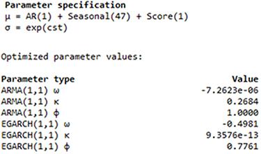
where φ(S)i, κ(S)j and ω(S) are the EGARCH parameters, while σ is the standard deviation (de la Fuente et al 2020). The specification of the parameters SAR(TVAR)[p,d,q] × [P,D,Q]m in equation (2), and EGARCH (P,0,Q) in equation (3), and their optimised values are given in figure 1A.
Figure 1A. Parameter specification and optimised values for the SAR(TVAR)-EGARCH (DMI) model.
Download figure:
Standard image High-resolution image
In terms of the variance equation, we find a symmetric effect, φi (S), which is significantly different from zero, while (κ(S)j ) is small and not significantly different from zero because the conditional volatility is not very persistent. Basawa et al (2004), Lit et al (2019–2023) provide additional numerical insights and solutions to equation (2).
The statistics in both the training and validation stages are promising (figure 2A, box). In particular, in the training stage, root mean square error (RMSE) and mean absolute error (MAE) are around 0.055, while the MAPE stands at 173, with a Log Loss of −1.3. Although the RMSE and MAE double in the validation stage, they still remain low, especially the MAE at 0.12. The lower performance of metrics such as MAPE and Log Loss can be attributed to their emphasis on outliers or specific aspects of the data, which might make the sub-model's performance appear poorer. Conversely, MAE and RMSE provide a more generalised measure of overall accuracy. It is important to consider the complete array of metrics presented in sub-section 3.3, as they collectively reflect the performance of the sub-model. Furthermore, the evidence from the comparison between the model with and without the DMI auxiliary variable indicates that the former outperforms the latter (sub-section 3.4).
DMI—model evaluation (1880–2021)
DMI—forecast (2022–2051)