
Abstract
Accurate observation of two or more particles within a very narrow time window has always been a challenge in modern physics. It creates the possibility of correlation experiments, such as the ground-breaking Hanbury Brown–Twiss experiment, leading to new physical insights. For low-energy electrons, one possibility is to use a Microchannel plate with subsequent delay lines for the readout of the incident particle hits, a setup called a Delay Line Detector. The spatial and temporal coordinates of more than one particle can be fully reconstructed outside a region called the dead radius. For interesting events, where two electrons are close in space and time, the determination of the individual positions of the electrons requires elaborate peak finding algorithms. While classical methods work well with single particle hits, they fail to identify and reconstruct events caused by multiple nearby particles. To address this challenge, we present a new spatiotemporal machine learning model to identify and reconstruct the position and time of such multi-hit particle signals. This model achieves a much better resolution for nearby particle hits compared to the classical approach, removing some of the artifacts and reducing the dead radius a factor of eight. We show that machine learning models can be effective in improving the spatiotemporal performance of delay line detectors.
Export citation and abstract BibTeX RIS

Original content from this work may be used under the terms of the Creative Commons Attribution 4.0 license. Any further distribution of this work must maintain attribution to the author(s) and the title of the work, journal citation and DOI.
1. Introduction
The detection of single particles, such as atoms, ions, electrons and highly energetic photons is the cornerstone of many fields in fundamental physics research. Typically, the signal due to a single particle is too faint to be measured directly and requires amplification. It is usually achieved with electron avalanches, as for example in Photon Multiplier Tubes [1] and Microchannel Plates (MCPs) [2]. MCPs offer the advantage that the incident particle can be spatially resolved with a phosphor screen or a wire-grid. The latter system is called a Delay Line Detector (DLD) [3], a spatially and temporally resolving detector, schematically shown in figure 1. DLDs can be used for ions, electrons and photons with energies high enough to emit an electron from the front side of the MCP.

Figure 1. Experimental setup for measuring multi-electron events with a Delay Line Detector. Triggered by ultrashort laser pulses, the needle tip emits one or more electrons that hit the Microchannel Plate (MCP), intensified by secondary electron emission. The resulting bunch passes the delay lines and induces a voltage pulse, producing the data for 6 channels (Ch1–6) and the MCP signal. After amplification the data is discretized by the analog-to-digital converter (ADC).
Download figure:
Standard image High-resolution imageIn ultra-fast atomic physics, DLDs are used for Cold Target Recoil Ion Momentum Spectroscopy [4], a technique for resolving the correlation of two simultaneously emitted electrons in non-sequential double ionization [5]. In another seminal experiment, a DLD was used to compare the bunching and anti-bunching behavior of free bosonic particles and free fermionic particles [6]. Usually the strength of correlation signals scales inversely with the separation of the particles, e.g. Coulomb interaction for electrons. Therefore, it is an important task to reconstruct particles that are as close as possible without errors. Despite the additional information provided by the three layers of delay lines, the disentangling of two or more incident particle signals becomes increasingly more challenging the closer the particles get to each other. Although DLDs are very effective in identifying and reconstructing single particle hits, they are much more limited in the ability to identify and reconstruct multi-hit events that are close in space and time. In such scenarios, the signals will significantly overlap and present reconstruction challenges.
Machine learning has seen an explosive increase in use in physics, including use cases for classification, regression, anomaly detection, generative modeling and others [7–15]. Most of these studies focus exclusively on the spatial or on the temporal domain. Recently, spatiotemporal studies and models that combine spatial and temporal input data have started gaining traction in physics and other fields [16–26]. For a review of deep learning spatiotemporal applications, please see [27]. Additionally, machine learning algorithms have recently been applied to the challenge of reconstructing close-by particles, for example, by the CMS Collaboration [28].
In this work, we focus on the particularly challenging scenario where the individual signals due to multiple particles are close in space and time. We show that machine learning algorithms can significantly improve the multi-hit capability of DLDs compared to classical reconstruction methods. Our approach can substantially reduce the effective dead radius of simultaneously arriving particles, improving the overall quality of the reconstruction.
The content of the paper is structured as follows: Section 2 explains the experimental setup of the DLD and data collection. In section 3 the classical peak finding methods are described, followed by the the machine learning approach in section 3.5. In section 4 we present the results, followed by their interpretation in section 5. Section 6 provides a summary and outlook.
2. Experimental setup
The experimental setup is shown in figure 1. It consists of a tungsten needle tip with an apex radius of  5–20 nm that is illuminated with ultra-short few-cycle laser pulses from an optical parametric amplifier system. It has a central wavelength of
  nm and a repetition rate of
  kHz. The typical pulse duration is
  fs. As the electron emission occurs promptly with the incident laser pulse, this represents an ultra-fast electron source with initial pulse durations of a few femtoseconds that are far below any electronically resolvable time scale.
The whole experiment takes place in an ultra-high vacuum chamber with a base pressure  mbar. The tip is typically biased with a voltage between
  to
to  V that corresponds to the final energy of the emitted electrons except the influence of the laser field. Due to the negative bias, the electrons are accelerated away from the tip and travel towards the delay line detector. In more detail, it consists of a Chevron type (double) Microchannel plate detector. The front MCP is a funnel-type MCP that provides a very high detection efficiency. Each incident electron will cause secondary emission, resulting in an electron bunch of 105–106 electrons. This electron bunch is additionally accelerated towards a biased meandering wireframe called the delay line.
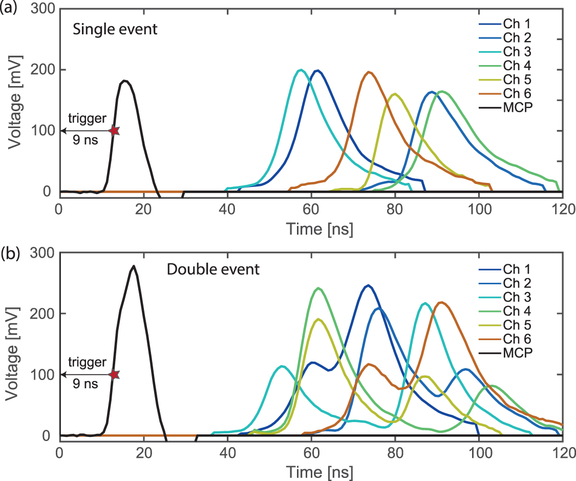
The electron bunch will induce a voltage pulse at the same position where the incoming particle has hit the MCP. Two voltage pulses are excited and travel in both directions in each wire of the wireframe and are detected at each end of the wire. There are three such wireframes behind the MCP, resulting in six channels where the signals are recorded. Additionally, a seventh voltage signal can be picked up from the supply voltage of the MCP with the help of a bias tee. In total, the detector output counts up to 7 signals that are fed out of the vacuum chamber, amplified and digitized by a fast analog-to-digital converter (ADC) with a bin-size of  ns. Typical single and double hit event time traces are shown in figure 2.
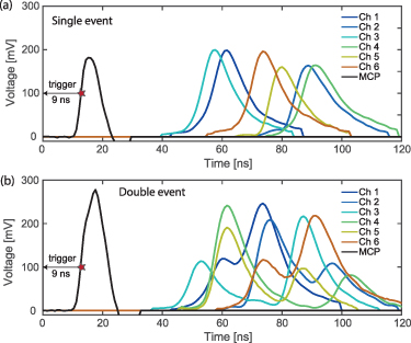
Figure 2. (a) Typical time trace of one electron hitting the Delay Line Detector. 7 channels are recorded, consisting of 6 delay line signals and one Microchannel Plate Detector signal. (b) Two-electron event, where two MCP peaks are merged into a single peak, as can be seen by the shoulder to the left. For each event, data recording starts 9 ns before the trigger threshold is reached, as indicated by the arrow and the red star.
Download figure:
Standard image High-resolution image3. Spatiotemporal signal reconstruction methods
The classical approach for analysis of DLD reconstruction data consists of two commonly used methods: the hardware-based Constant Fraction Discriminator (CFD) and the Fit-based Method (FM).
3.1. Hardware-based time stamp detection
For commercial DLDs, the determination of the  information for the incoming particles relies on a hardware-based detection of the time stamps from the anodes and the MCP, combined with an evaluation software. In commercial DLDs, the signals are fed into a CFD after amplification. The CFD principle works as shown in figure 3: an incoming signal is superimposed with its copy that was electrically reversed and reduced by a factor of about 3. Additionally, the original signal was shifted in time, which results in a well-defined zero crossing that defines the point in time where that specific signal arrived. To determine the zero crossing purely electrically, two comparators are used: (1) one that gives a logic level one when a certain threshold is exceeded, while (2) the second one gives a logic one when the signal is above the zero-voltage level (noise-level). The time-stamp is given by the point where both comparators are one. The advantage of this method is that it is independent of the actual pulse height. The CFD outputs a Nuclear Instrument Module (NIM) pulse with a well-defined shape whose rising flank is at the temporal position of the peak of the original signal. This NIM pulse is detected by a time-to-digital converter that digitizes the timing information with a resolution of
  ps. We will refer to this approach as the CFD method.

Figure 3. Principle of the constant fraction discriminator (CFD): An incoming pulse is split into two parts. The upper one is delayed, the lower one is inverted and multiplied by a factor  . Both pulses are combined and sent into two comparator circuits. A NIM pulse is created whose rising edge contains the time information.
Download figure:
Standard image High-resolution image3.2. Multi-hit capability of the hardware-based time stamps
The time tags produced by the CFD method are robust, fast and easy to handle. However, their multi-hit capability is limited when it comes to close-by events. As shown in figure 4, two equal peaks will result in only one zero crossing as soon as they are closer than 1.9 times their Full Width at Half Maximum (FWHM). In absolute numbers, as the signals propagate with an average speed of 0.9 mm ns−1, this leads to an average dead radius of 21 mm, as the FWHM of the norm-pulse
3
is  ns. Even before the dead radius is reached, errors on the reconstructed peak positions occur, as shown in the white area in figure 4(a). If two particles hit the detector with a spatial distance smaller than the dead radius, only one particle will be reconstructed. Its position will also be subject to error, as shown in figure 4(c). The second particle will have even larger errors, as can be seen in figure 4(d). The relative amplitude difference of the two peaks matters. If the distance between two particles is smaller than the dead radius, this shift is even more pronounced, and will result in one registered particle, as indicated by the white area in figure 4(d) where no detection is possible.
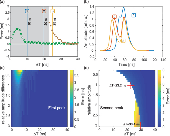
Figure 4. (a) Error of Constant Fraction Discriminator (CFD)-based double-hit evaluation. Below  ns only one peak position can be found. The green data show the error of the first peak, the brown of the second. The curve was created by application of the CFD principle to a norm pulse in a simulation. The gray area shows the time differences where the CFD only finds one peak. (b) Different examples of double hits, created by the sum of two norm pulses with a time delay of 10 ns (blue, 1), 20 ns (orange, 2) and 25 ns (yellow, 3). Their respective governed peak positions are shown in (a). In both (a) and (b) the amplitudes of the two peaks were equal. (c) Error of the first peak as function of relative peak height difference and time difference Δt. (d) Same map as (c) but now for the second peak. The white area means that no second peak was found.
Download figure:
Standard image High-resolution image3.3. Analog data readout for improved classical model evaluation
For applications that require better multi-hit capability compared to the basic hardware-based method, it is possible to purchase and use fast ADC cards to digitize each analog trace and use computer-based algorithms to obtain the timing information. The ADC cards have a data rate of 300 MB s−1 providing a theoretical measurement speed of  kHz, assuming an average data length of
  bins. After the data is recorded, we perform an offline data evaluation following the measurements using MATLAB [29] and Python [30] to analyze the events. The software of the ADC cards will split multiple events on a single channel if they are separated long enough that the amplitude is lower than a pre-set trigger threshold. In this case, we first run a routine that interpolates all parts of each channel to the same time grid. In the next step, we use a peak finding algorithm in MATLAB. This classical algorithm searches for the indices of peak maxima and performs a fit on a window around them.
In figures 5(a) and (b), the classical algorithm is used to generate the first and second peaks, with the graphs displaying the errors of these peaks as a function of their separation. We tried different functions and selected the skewed normal distribution due to its superior performance. The fit window is 5 bins to the right and left. If another peak is closer than 20 bins, the window is shrunk to 2 on each side and the fit function is changed to a quadratic function. The peak positions are passed to a position calculation software that reconstructs the event and finally calculates the position ( ). We call this approach fit-based classical method.

Figure 5. (a) Absolute error on the first peak for a constructed double hit using two norm pulses evaluated with the fit-based classical algorithm. (b) Absolute error on the second peak by the fit-based classical algorithm.
Download figure:
Standard image High-resolution image3.4. Mean pulse curve fit
This method is motivated by [31–33]. Shifting and scaling single hit signals to the same position and height allows the extraction of a 'mean pulse'. One can then fit the double peak signal to a sum of two mean pulses to reconstruct the two peaks. We call this method the 'mean pulse curve fit' (MPCF). The mean pulse can be seen in figure 6. In figure 6(a) it is shown that Channels 1–6 have a very similar mean pulse, only the MCP mean pulse has a different form. Thus, we combined channels 1–6. Figure 6(b) shows 10k signals from channels 1–6 (gray) and their mean (red). Each signal consists of a fixed number of points, in our case this is 153 time bins. In order to be able to shift the mean pulse on a sub-bin level, the mean pulse is interpolated. The fit function then consists of a sum of two interpolated mean pulses, each shifted, scaled and stretched. There are six fit parameters, ![$[x_0, x_1, h_0, h_1, s_0, s_1]$](https://content.cld.iop.org/journals/2632-2153/5/2/025019/revision2/mlstad3d2dieqn17.gif) , the peak positions xi
, the peak heights hi
and the peak stretches si
,
, the peak positions xi
, the peak heights hi
and the peak stretches si
,  . Using the curve_fit function in scipy.optmize [34] the six fit parameters are determined. The fit is initialized with random parameters.

Figure 6. Calculation of the mean pulse. Because the mean pulses of channels 1–6 are so similar (a), we combined them to one mean pulse (b).
Download figure:
Standard image High-resolution imageThe quality of the fit depends upon the initial conditions and often the outcome is visibly wrong. Several improvements are needed. First, bounds are added to the fit parameters. For the positions xi
the bounds are the x-interval, in this case ![$[0,153]$](https://content.cld.iop.org/journals/2632-2153/5/2/025019/revision2/mlstad3d2dieqn19.gif) . Further we restrict the heights hi
to
. Further we restrict the heights hi
to ![$[0.15 h_\mathrm{max}, 1.25 h_\mathrm{max}]$](https://content.cld.iop.org/journals/2632-2153/5/2/025019/revision2/mlstad3d2dieqn20.gif) , where
, where  is the maximal value of the given signal. Limiting the amplitude, especially in scenarios with closely spaced peaks, is beneficial. This is because a single average pulse can often provide a good fit, leading to the second peak's amplitude going to zero. With similar reasoning, the stretch is constrained to
  . Additionally, upon executing the fit using the mentioned scipy function, we assess the root mean square error (RMSE). If this RMSE surpasses a predefined threshold,
  , we reinitiate the fitting process with a new set of randomly chosen initial parameters.
  is initially set at 3% of
  . Following 13 unsuccessful attempts, the threshold
  is incrementally increased by a factor of 1.15 each time the fit failed to be better than the current
  .
.
A better way of initializing the fit parameters is to perform a fast peak finding algorithm on the signal. We use the argrelextrema function in scipy to get the positions of the relative maxima in the signal. Since the fit often does not fulfill the  bound and to have more attempts with slightly different initial conditions, we take the initial positions xi
by sampling from a normal distribution with the outputs of argrelextrema as the means and a variance σ that increases with every attempted fit, starting with σ = 20. The initial heights hi
are sampled from a normal distribution with mean
bound and to have more attempts with slightly different initial conditions, we take the initial positions xi
by sampling from a normal distribution with the outputs of argrelextrema as the means and a variance σ that increases with every attempted fit, starting with σ = 20. The initial heights hi
are sampled from a normal distribution with mean  and variance
  . The initial stretches si
are also randomly sampled from a normal distribution around 1.0 with variance 0.3. Lastly, after evaluation of the MPCF method on simulated double peak signals, we found that the MPCF had a general bias in one direction. We find the peak positions of 10k simulated doubles with the MPCF and calculate the mean error by comparison with the true peak positions. In our case the bias was −0.53, meaning
. The initial stretches si
are also randomly sampled from a normal distribution around 1.0 with variance 0.3. Lastly, after evaluation of the MPCF method on simulated double peak signals, we found that the MPCF had a general bias in one direction. We find the peak positions of 10k simulated doubles with the MPCF and calculate the mean error by comparison with the true peak positions. In our case the bias was −0.53, meaning  was on average −0.53. To compensate, we subtract this bias from all predictions made by the MPCF method.
Examples of predictions using the MPCF method are shown in figure 7. The MPCF is performed on data simulated from two random real single hit signals. The mean pulse used for fitting does not exactly match the shapes used for generation. Thus, for closer signals, the MPCF starts deviating from the ground truth, see the bottom plot in figure 7.

Figure 7. Three examples of predictions from the mean pulse fit method. Top: Far apart peaks, middle: close, but still two peaks visible, bottom: close and only one peak visible. Gray: actual pulses/peaks, red: predicted pulses/peaks. The actual pulses all have the same amplitude.
Download figure:
Standard image High-resolution image3.5. Machine learning approach
The machine learning approach that we use to identify and reconstruct multi-hit events for DLDs consists of multi-hit data generation, a Hit Multiplicity Classifier (HMC) and Deep Double Peak Finder (DDPF). It is summarized in figure 8.
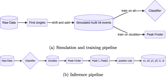
Figure 8. (a) Simulation and training pipeline: real singles are shifted and added to create simulated multi hit events for classifier and peak finder training (b) inference pipeline: the classifier determines if the event has one, two, three or four hits. For the double hit events, every channel is fed separately into the Deep Peak Finder model.
Download figure:
Standard image High-resolution imageSimulation and training workflow: The raw analog data is preprocessed for each event, including analog to digital conversion and zero-padding to ensure a constant vector length. From real single particle events, we generate multi-particle hit events, including doubles, triples and quadruples and use them to train a HMC to distinguish among the different hit multiplicity events. Next, we train a DDPF model to predict the peak positions for double events, as shown in figure 8(a).
Inference workflow: After the data is pre-processed, we apply the HMC model to classify the events into singles, doubles, triples and quadruples by using 6 out of the 7 channels (excluding the MCP channel). Next, we apply the DDPF model to the classified events to identify the peak positions for each channel. These peak positions are passed to a position calculation software that matches the peaks and reconstructs the event. The final outputs are the x and y positions, as well as the time t for each particle as shown in figure 8(b). Our approach is general, and can be applied to any hit multiplicity once the classifier is applied. We restrict ourselves to the analysis of double-hit events for a detailed evaluation and comparison with classical methods and leave further studies of higher multiplicity events to future work. For single hit events classical algorithms work well, and no machine learning models are necessary.
3.5.1. Multi-hit data generation
As the voltage signals of events are approximately additive, as can be seen in figure 9, it is possible to simulate multi-hit events through addition of single peak signals to obtain doubles, triples and quadruples. The advantage of this approach is the exact knowledge of the individual peak positions without any shifts caused by a secondary hit. To obtain the single peak events needed for the simulated multi-hit events, we use the following filtering strategy:
- We first employ the classical peak finder algorithm. Events with multiple peaks in any channel are excluded.
- Each event is normalized by dividing the values in each channel by the event's maximum value. We then aggregate the values across all channels for each event to compute a unique metric, termed the 'event area'. Events exceeding a threshold of the mean area plus a constant factor are discarded. They are probably double or triple hit events which could not be distinguished by the classical algorithm.
- Using the remaining single hit candidates, doubles, triples and quadruples are simulated and an intermediate classifier model is trained on them. This classifier is then employed to further refine the remaining events.

Figure 9. Examples of real double hits in different channels compared to constructed simulated double hits. Blue: real measured double hit, red: single hits that have been shifted and scaled so that their sum corresponds to the real double hit. Black dashed line: simulated double hit from the addition of the singles.
Download figure:
Standard image High-resolution imageAlthough this process can be iterated, we observe that additional iterations beyond the first do not significantly alter the remaining events. To create data for the HMC, random events undergo simultaneous shifts in time in all channels (with one random shift for each event) and are then added across all channels concurrently. To simulate double-hit signals for the DDPF, two single-hit signals are randomly shifted in time and added. The shifting ensures that the model also sees peaks in regions where single hit signals might not show peaks, but in actual double hit signals, peaks would be present. The peak positions in the generated events are known up to the same accuracy as for the single-hit events. Since the peak finder model predicts the peaks for each channel separately, we simulate double events for each channel separately and then shuffle the data of the different channels.
Figure 9 shows two typical real and simulated double peaks. The real and simulated doubles look almost identical except at the edges of the signals that are far away from the center of the peaks. These parts of the signals are less relevant as they do not contain additional timing information of the peaks.
3.5.2. HMC
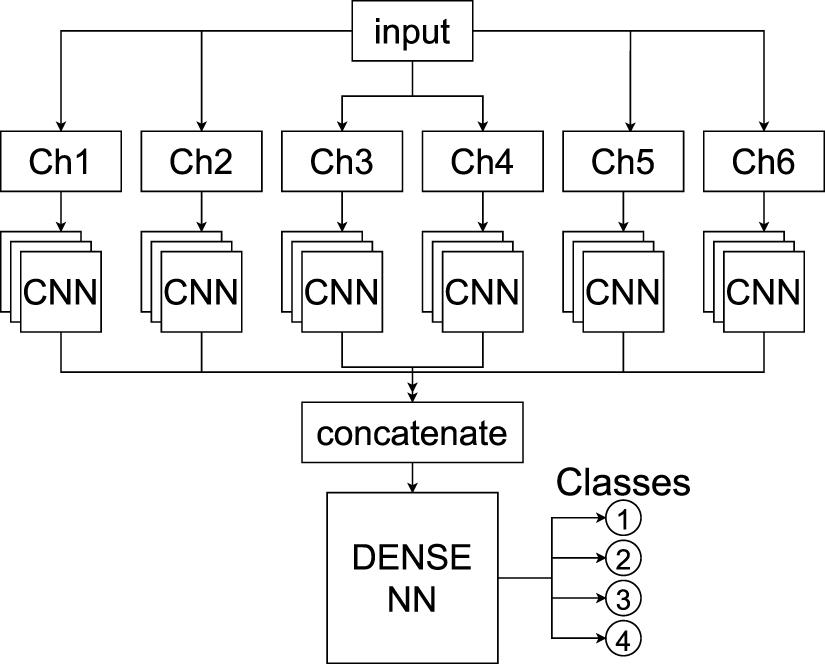
A sketch of the HMC is shown in figure 10. The input amplitudes are normalized on an event basis and split into 6 channels. Each channel is passed to a 1D convolutional neural network (CNN) that consists of: [Conv1D, BatchNorm, ReLu, Conv1D, BatchNorm, ReLu, GlobalAveragePooling] layers. The hyperparameters num_filters and kernel_size are optimized during training. After flattening, the outputs of the CNNs get concatenated and go through a dense neural network with [Dense, Dropout, Dense, Dropout] layers, where the number of neurons, dropout and activation are hyperparameters. The last layer has 4 neurons, one for each class, with softmax activation outputs.
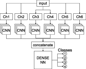
Figure 10. Hit Multiplicity Classifier model structure: The input is split into the channels Ch1–6 (without MCP) and each channel separately goes through a 1D CNN. The outputs of the CNNs are concatenated and put through a simple dense NN. The output of the dense NN are the probabilities for the classes [1,2,3,4].
Download figure:
Standard image High-resolution image3.5.3. DDPF
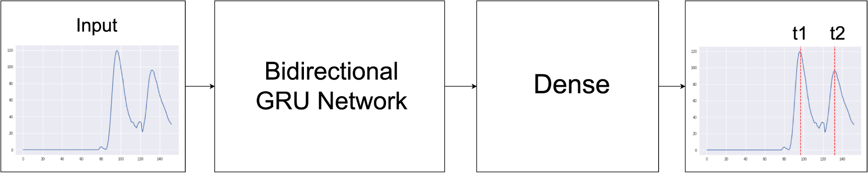
A sketch of the DDPF model for double-hit events is shown in figure 11. Using data from one of the six channels at a time (without MCP), the model predicts two peak positions. The signal amplitude is normalized for each signal and passed into two bidirectional Gated Recurrent Unit (GRU) layers [35]. If the second GRU layer returns sequences, its output is flattened. A GRU is very similar to a long short-term memory (LSTM) network [36] cell with a forget gate. A sketch of a GRU can be seen in figure 11. We use a bidirectional GRU, i.e. the model steps through the time series in both directions. Next, a set of [dropout, dense] layers is used. A dense layer with 2 output neurons with sigmoid activation, one for each peak, produces the output of the network. We use the sigmoid activation function because the peak positions are scaled to [0,1].

Figure 11. Deep Peak Finder model structure: The model operates on single channel data. After a bidirectional GRU network, a dense network predicts the two peak positions.
Download figure:
Standard image High-resolution image3.5.4. MCP deep double peak finder
The MCP signals have a slightly different shape and a reduced signal width compared to the other channels. Therefore, a separate model is trained for the MCP. Single events are shifted and added to create simulated doubles. The MCP model has the same structure that is described above. The model's hyperparameters are tuned during training on simulated MCP doubles.
3.5.5. Training protocol
For each model, we performed hyperparameter tuning on a smaller dataset using Keras Tuner [37] and the Hyperband optimizer [38]. Models with the best hyperparameters were retrained on the full dataset.
The HMC model is trained with categorical cross-entropy as the loss function. The optimal hyperparameters were: activation: 'relu', dense_1: 132, dense_2: 144, dropout: 0.4, kernel_size_1: 17, kernel_size_2: 17, learning_rate: 0.01, num_filters: 55. After hyperparameter optimization, we retrained the best model for 300 epochs on 400k events (100k per class) using early stopping, keeping the best model based on validation loss and reduction of learning rate on plateau.
For the DDPF model for channels 1–6, we use mean square error (MSE) as the loss function. The optimal hyperparameters were: GRU_units: 70, activation: selu, clipnorm: 0.001, dropout: 0.2, hidden_layer_dim: 100, learning_rate: 0.001, num_layers: 1, ret_seq: 0. The best model was then retrained on 1 M simulated doubles for 300 epochs with a batch size of 128.
The MCP DDPF model has the same setup and MSE as the loss function. The optimal hyperparameters were: GRU_units: 65, activation: selu, clipnorm: 0.001, dropout: 0.2, hidden_layer_dim: 170, learning_rate: 0.001, num_layers: 1, ret_seq: 0.
4. Results
4.1. Hit multiplicity classifier results
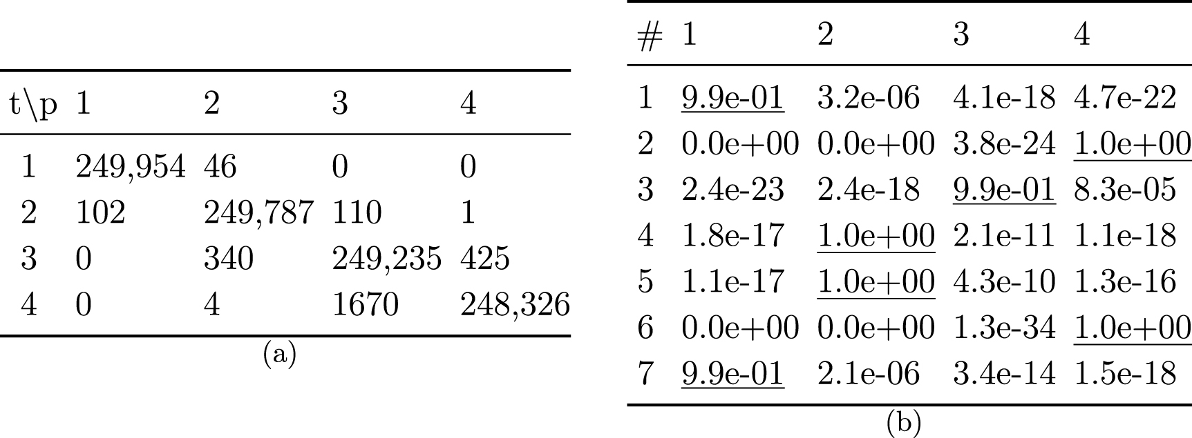
The Hit Multiplicity Classifier model has a test accuracy of 0.9973. for the test data consisting of 1 M events evenly split into singles/doubles/triples/quadruples. The area under the ROC curve (AUC) is  for every class (one-vs-all) and thus also for the macro average. The respective confusion matrix and example predictions are shown in figure 12.

Figure 12. (a) Confusion matrix (true\predicted) for the Hit Multiplicity Classifier tested with 1000 000 evenly split test events. (b) Hit Multiplicity Classifier probabilities (trunkated at 2 digits) for some random events. The most probable event class is underlined. All given events were predicted correctly. As can be seen from the confusion matrix, the classifier is very accurate, which results in the very high area under the curve (AUC) of  (one-vs-all).
Download figure:
Standard image High-resolution image4.2. Deep double peak finder results (channels 1–6)
On the training data, the root mean square error (RMSE) is  and the mean average error (MAE) is
  . Evaluated on 6 M simulated double-hit events, the final model has an RMSE for the peak position
  and the MAE is
  . The bin size of the data is 0.8 ns.
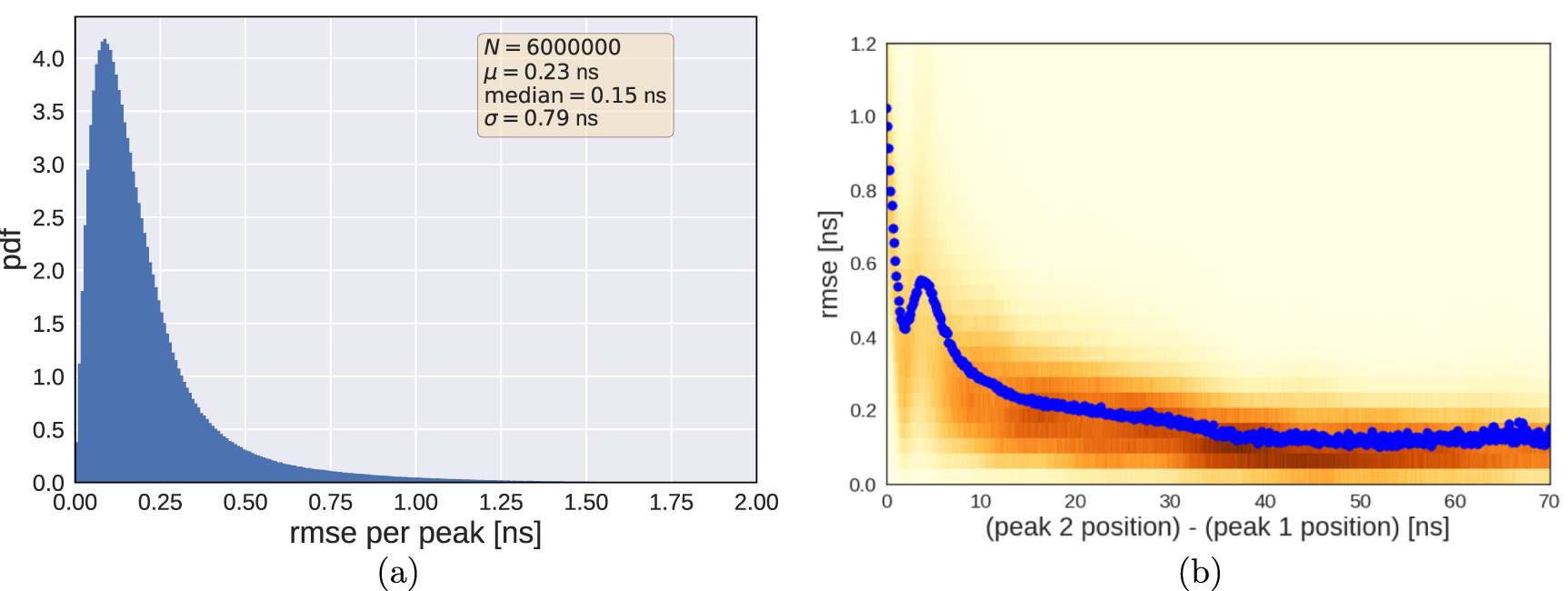
Figure 13 shows the error distribution on 6 M simulated double peak signals from all six channels (no MCP). We observe an overall small error below 0.3 ns for peaks separated by more than 10 ns and an error below 0.6 ns for closer hits. The mean error increases for smaller peak distances as well as the variance. Closer peak positions are more difficult to determine, which is to be expected. Figure 14 shows simulated double hit signals with their underlying single hit signals. Once the peaks get close enough, the position of the two underlying peaks will usually no longer coincide with the maxima of the curve.

Figure 13. Deep Double Peak Finder (without MCP): (a) RMSE distribution. (b) RMSE as a function of the peak distance. Performance of the peak finder model on 6 M simulated double hit signals from all six channels. In (b) the background shows the 2D histogram normalized such that each column adds up to 1 and the blue dots show the mean at the respective peak distance.
Download figure:
Standard image High-resolution image
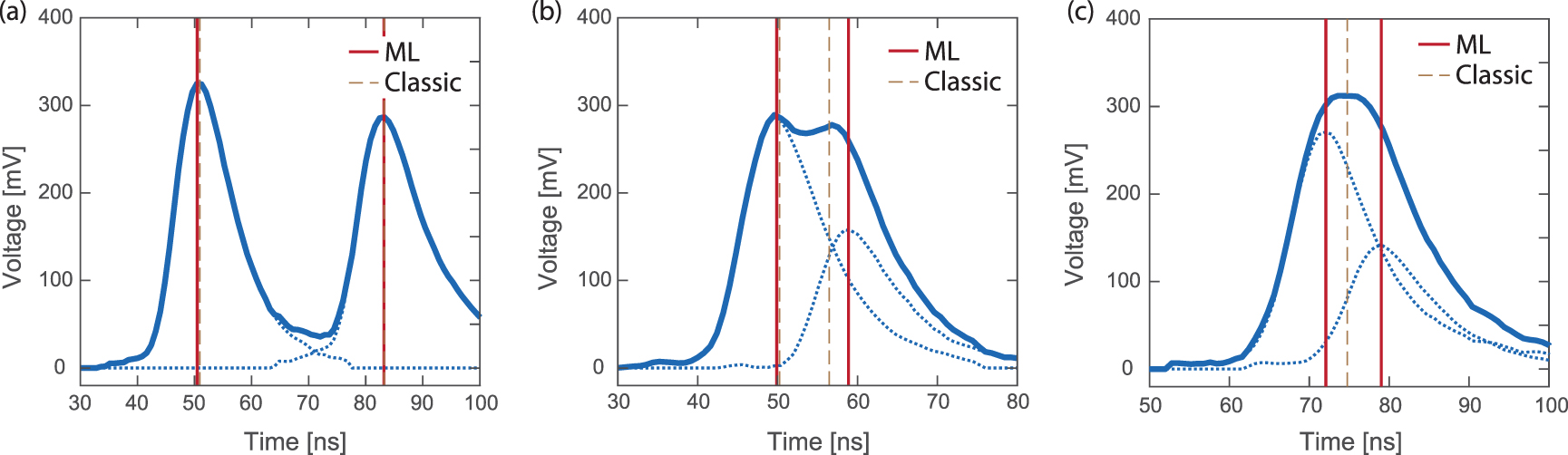
Figure 14. Example events with simulated constructed double events. Thick blue line: the data that the classical and the machine learning algorithm received. It consists of the two thin blue lines, so in this case we can exactly know where the peaks should be. (a) Event with two distinct peaks. The classical as well as the machine learning algorithm can capture both peaks well. (b) Event with two close peaks: the classical algorithm still sees two peaks, but they are reconstructed in at the wrong positions as both traces strongly overlap. (c) very close event: the machine learning algorithm is still capable to find both peak positions, while the classical algorithm only finds one maximum which is not at any of the real peak positions.
Download figure:
Standard image High-resolution image4.3. Deep double peak finder results (MCP)
The test data consists of 6 M simulated MCP double peak signals and the root mean square error is  and
and  . The mean average error is
  and
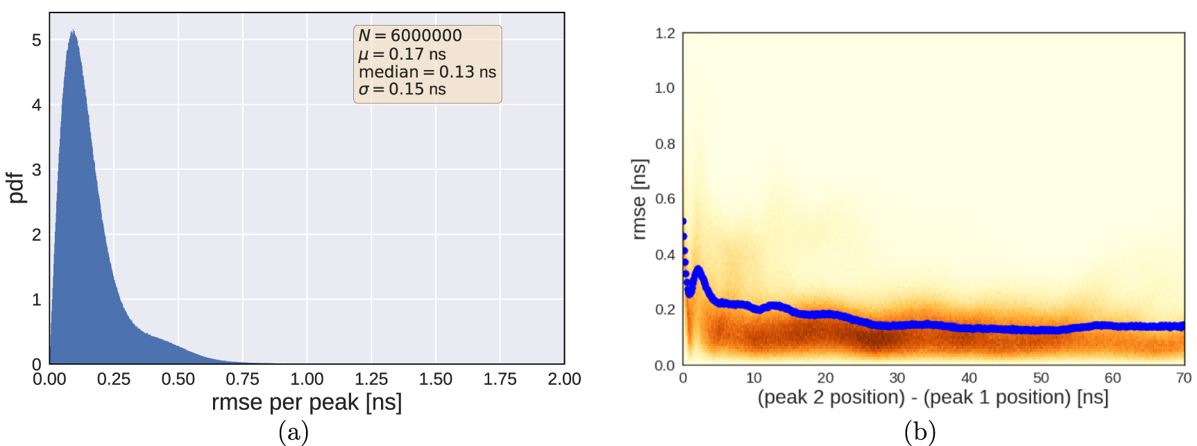
and  . The bin size of the data is 0.8 ns. Figure 15 shows the RMSE distribution (a) and the RMSE as a function of peak distance (b). The performance of the MCP model is better than the performance of the general deep double peak finder model from figure 13.

Figure 15. Performance of the MCP only Deep Peak Finder model on simulated test data: (a) Root mean square error distribution. (b) Root mean square error as a function of the peak distance. The test data consists of of 30k simulated doubles. In (b) the background shows the 2D histogram normalized such that each column adds up to 1 and the blue dots show the mean at the respective peak distance. The mean error increases for smaller peak distances as well as the variance. Closer peaks are more difficult to accurately determine, which is to be expected. The outliers come from not enough data for the respective bin, where one single bad prediction strongly influences the mean.
Download figure:
Standard image High-resolution image4.4. Comparison between classical and machine learning reconstruction models
In figure 16, we compare the machine learning model (6 channels) to the fit-based classical algorithm described in section 3.3. The test data consists of 3 M generated signals from channels 1–6. We filtered the data such that no peaks are closer than 16 ns to one of the borders of the interval, because most methods do not work when a large part of the peak is cut off. For the error bars we fit a function to the error distribution in each peak separation bin. The error bars correspond to one standard deviation of the fitted distribution. We tested different functions and a Rayleigh distribution worked most consistently across all peak separations.

Figure 16. Log plot of the root mean squared error as a function of the peaks separation for the channels (not MCP). The green region is where the fit-based method has a smaller error, the red region is where the Deep Peak Finder has a smaller error.
Download figure:
Standard image High-resolution imageThe classical model (shown in green) performs almost perfectly for distances  . This is exactly as expected, as the labels were created using the classical algorithm to find the singles and their peak positions. For peak distances smaller than around
  (about the width of the peaks), the error of the classical model significantly increases, while the machine learning model performance only slightly degrades. For much closer peaks, the classical algorithm becomes better again. This also makes sense, as the classical algorithm only predicts one peak once the two peaks have merged. If the peaks merge to one peak at exactly the same position, then the classical algorithm gives the correct result again (accidentally), without knowing that there are two peaks. The same applies to the CFD method and the decrease in RMSE for peak separations closer than 10–20 ns for CFD and fit-based is purely this effect. If all the signals where only one peak is predicted are dropped, then this effect goes away.
The huge difference between RMSE and MAE in the peak finding models comes from few very large errors, as RMSE puts a higher weight on large errors. If we take out all data points where the error is larger than  , which amounts to 0.4% of the data, then
  and
and  . If the position calculation software cannot reconstruct the event, it is typically discarded. The higher test loss than training loss indicates some amount of overfitting. Increasing dropout did not increase model performance on validation data.
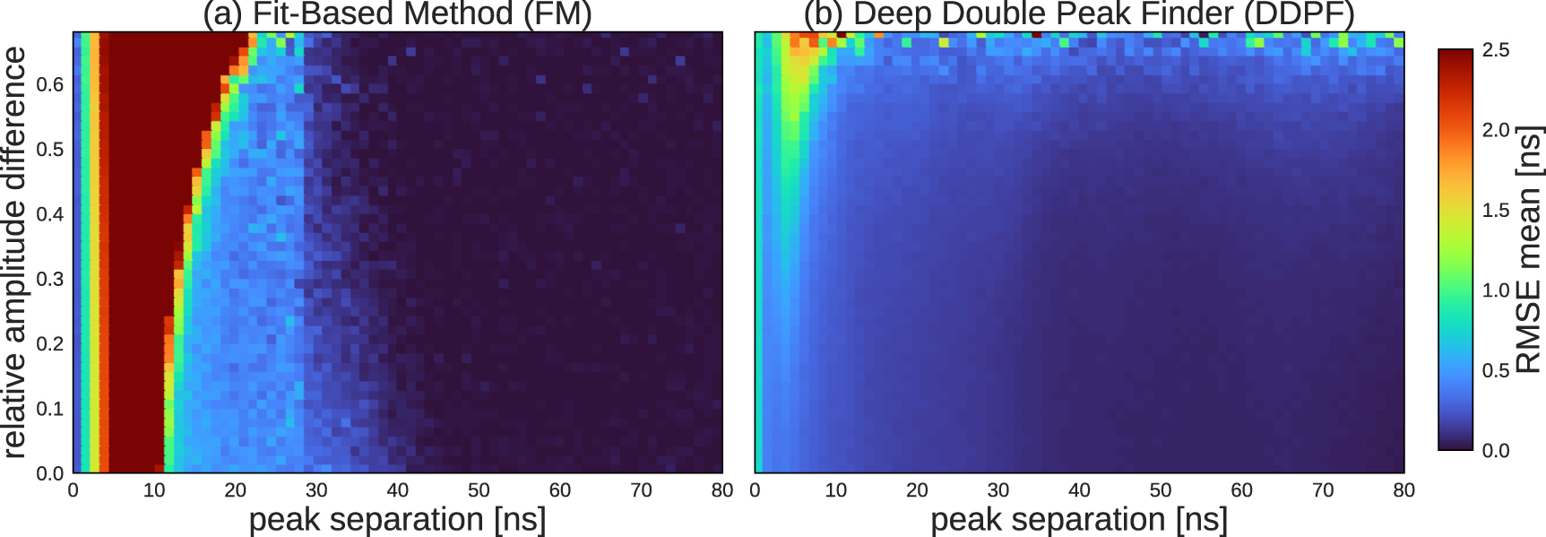
The performance of the models not only depends on the peak separation, but also on the amplitudes a0 and a1 of the underlying signals. Two peaks of about the same height can get closer to each other without merging to a single peak than two peaks with very different heights can. In order to investigate the performance of the models with respect to the differences in amplitudes, we introduce the 'relative amplitudes difference' metric:  . Figure 17 shows a plot where the peak separation and the relative amplitudes difference are on the x- and y-axis and the color shows the mean of the RMSE distribution for the respective bin.

Figure 17. RMSE mean (color) as a function of peak separation and relative amplitudes difference. (a) Fit-Based Method, (b) Deep Double Peak Finder.
Download figure:
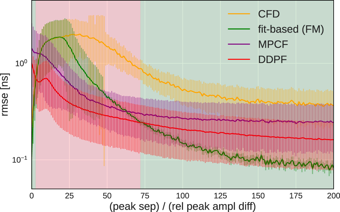
Standard image High-resolution imageWe can now introduce a function of the peak separation and the relative amplitudes difference and reduce the plots in figure 17 to two dimensions. We introduce

motivated by the premise that it is hard to predict the peak positions when a) the peaks have a small separation and b) when the relative amplitudes difference is large. Thus the region with small ξ is hard to predict and the region with large ξ is much easier to predict, as shown in figure 18. Constant ξ corresponds to a straight line through the origin in the  -
- -plane and a point in figure 18 corresponds to the mean along the respective line. The error bars are from fitting a Rayleigh distribution to the RMSE distribution in the respective ξ-bin and taking one standard deviation of the fitted distribution.

Figure 18. RMSE comparison between the different methods as a function of  . The green region is where the fit-based method has a smaller error, the red region is where the Deep Peak Finder has a smaller error.
Download figure:
Standard image High-resolution image4.5. Real data inference
As a final check, we compare the classical evaluation methods that are given by the hardware-based CFD peak retrieval method and the fit-based classical method to the results we obtained with the machine learning models described in section 3.5 using real data. The following evaluation and the given dead-radii are for true simultaneous double hits, meaning most electron pairs arrive within one ns. If the arrival time of the particles is widely spread out, also the dead-radius will get smaller as the particles can get distinguished by the time of flight and their signals will generally overlap less. We perform a measurement in which a copper grid, commercially available for sample preparation in transmission electron microscopy, is placed in front of the electron source as shown in figure 19. The shadow image of the grid is projected on the DLD, as shown in figure 19(a). Thus, there are sharp spatial features, either in real space for the first and the second electron, but also for the difference plots in which Δy is plotted over Δx for the double hits. The clarity of the grid appearing in the reconstructed positions and difference plots is an indicator for the quality of the method's performance. In the center of these images, a white circle with white lines is plotted that shows the dead region of the DDPF that we cut out in all four cases. In this region, it is not possible anymore to distinguish between two hits of low amplitude or one hit of large amplitude, which is why there errors will occur.

Figure 19. Position difference plots for data with a grid in front of the detector, casting a clear and regular electron shadow on the detector. Δx is  , where xi
is the position of particle i,
, where xi
is the position of particle i,  respectively. (a) Schematic display of the experimental setup. (b) positions from Constant Fraction Discriminator method, (c) positions from fit-based classical algorithm, (d) positions from the machine learning model with the Deep Double Peak Finder model, (e) 'ideal' plot purely from two uncorrelated singles. The two white circles indicate 10 mm and 20 mm on the images for comparison. The inner white circle with the white dashed area corresponds to the dead-area of the DDPF.
Download figure:
Standard image High-resolution image
Figures 19(b)–(e) shows the position differences, i.e. a 2D histogram of the x and y distances of the two particles. Figure 19(b) shows double hit events evaluated with the CFD-method. There is a star-shaped dead region (black region) with a maximal extension of about  where most events cannot be reconstructed. There are also other weaker 6-fold artifacts. Figure 19(c) shows double hit events evaluated with the fit-based classical peak finding algorithm. There are strong 6-fold artifacts, too, and the dead radius is at about
  . The strong hexagonal artifacts originate from the increasingly poorly determined peak positions as soon as the two signals come very close to each other, as shown in figure 14. The associated signals of the individual electrons on the different layers cannot be clearly assigned by the evaluation software, which subsequently leads to these artifacts. Figure 19(d) shows the same double events evaluated with the DDPF. While some remaining 6-fold artifacts are still visible, they are much weaker now compared to the classical methods in (b) and (c). d decrease the dead radius to a much smaller value of
  mm and the grid appears much sharper in the region closer to the center.
Figure 19(e) shows the difference between two single hit events. This is an 'ideal' plot obtained from two uncorrelated single hit events, showing a very good resolution of the grid. There, no intrinsic dead radius or other double-hit based detector artifacts as well as possible physical correlations are present.
The absolute numbers for the dead radius entirely depend on the FWHM of the pulse, here 12.5 ns (evaluated for a typical norm pulse). If the width of the norm pulse can be reduced by half through hardware changes, for example, then all dead radii can also be reduced by half, both those of the hardware-based evaluation and those of the classical algorithm as well as the machine-learning-based evaluation. This can be seen in the original article to the multihit capability of the DLD, see [39], where the authors obtained a FWHM of the pulses of 4–5 ns, thus already obtaining a dead radius of  mm. Since our evaluation enables a relative improvement compared to the peak width, such a signal width would also further improve our dead radius. Typically, also the particle species can influence the peak width, e.g. it should be smaller for ions.
5. Interpretation and discussion
As expected, the worst results are obtained using the hardware-based peak detection method with the CFD method. There is only one detectable zero crossing when two peaks come too close to each other. Therefore, we expect a large dead radius, which we observed in the difference plot in figure 19(b). Additionally, the grid is barely visible in this plot. By comparison, in figure 19(e), we see how the difference plot would look like for perfectly resolved double hits: the grid in real space results in a nicely observable pattern in the difference plot.
For peaks that are far enough apart, the fit-based classical algorithm is perfect and beats the DDPF, since the peaks do not influence each other and the labels were created with help of the classical algorithm as shown in figure 16. However, the difference between the machine learning model and the fit-based classical algorithm for well separated peaks ( ns) is on the order of 1/4 of the bin size (see figures 13(a) and 15(a)) and so the machine learning model still performs reasonably well in this regime. Once the peaks get closer they can influence the peak positions of the added signal. The peaks typically have a mean width of 12.5 ns (FWHM), so when the temporal separation comes close to this width, we expect the peak finding to become harder for the classical methods as well as for the machine learning model, as shown in figure 14(b). Already starting from 25–30 ns separation and below, we see an increase in RMSE in figure 16 for the classical method and the machine learning model performs visibly better below 25 ns. If the peaks get close, it often happens that there is only one single maximum in the added signal (figure 14(c)). The merging into one single maximum depends on the distance between the peaks and also the two amplitudes, so no hard threshold can be given. Below ≈10 ns peak separation the RMSE of the classical method strongly increases in figure 16. We also see it in the right panel in figure 14. The classical algorithm only finds one peak, whereas the machine learning model finds two peaks that fit well to the underlying peaks. Only for the case where the two peaks almost are on top of each other, below a distance of 1 ns in figure 16, the classical algorithm performs better again. This is expected since the classical algorithm finds the one peak and it is treated as two at the same position, while the ML model tries to find two peaks that would fit. Note that here the classical algorithm succeeds accidentally, as it believes there is only a single peak. Even in this region, the machine learning model performs well and the error is close to or below the bin size. Overall, the machine learning model performs better that the classical methods for peaks that are closer than 25–30 ns separation down to 1 ns. How easily the peak positions can be determined not only depends on the peak separation, but also on the relative amplitudes of the two underlying peaks as illustrated in figures 17(a) and (b). The fit-based method performs better for far peak separations for all values of the relative amplitude difference, at closer peak separations it gets very inconsistent, whereas the DDPF has a much smoother RMSE-mean-surface and stays lower and more consistent for closer peak separations. Combining peak separation and relative amplitude difference to a single variable ξ, figure 18 also shows that for
  [ns] the DDPF outperforms the other methods. Again, for ξ < 2.7 [ns] the fit-based method's rmse spuriously drops drastically, since here it only predicts one single peak and we had to take it as a double peak at this position in order to do this evaluation.
Furthermore, based on the grid plots obtained with real data in figure 19, it is clear that the DDPF model performs better than the classical methods on real data, showing a much smaller dead radius, less artifacts and better resolution compared to classical methods. While this was to be expected from the comparison between real and simulated doubles in figure 9, the grid plots further confirms this conclusion.
Note that in our exploration of various architectures, the CNN demonstrated notable efficacy as a classifier. However, its performance in peak detection tasks was less than satisfactory. Models based on GRUs exhibited superior performance in identifying peak positions. The use of LSTM) networks, instead of GRUs, did not yield any discernible improvement in our tests.
6. Summary and outlook
This paper presents a proof of concept for improving multi-hit capabilities of delay line detectors using machine learning. To our knowledge, it is the first time that the spatial and temporal resolution of a delay line detector has been improved with the application of machine learning algorithms.
We have shown that a machine learning approach that consists of Hit Multiplicity Classifier and DDPF models performs well on simulated and real data. The machine learning model finds the correct peak multiplicities and peak positions to a good accuracy even when classical methods fail to identify multi-particle hits. The models were also evaluated on real data using the grid approach as a point-projection image with an ultrafast low-energy electron source. This measurement, summarized in figure 19, can serve as a figure of merit for the quality of two-electron event evaluation on real data. It shows that our machine learning model surpasses the classical algorithms notably by having a smaller dead radius, fewer artifacts and a better resolution of the grid.
The current machine learning model is trained to identify multilple hit signals and only reconstruct double hit signals. The Hit Multiplicity Classifier already works up to quadruple hits with AUC  . In future follow-up work, we plan to extend the Deep Peak Finder to triple and quadruple events. We expect that our general method—generating multi-peak data through addition of singles, using a classifier followed by a peak finder for the specific multiplicity—will work for all or most applications where the signals are additive or approximately additive.
As this evaluation is applicable for any existing delay line-based detector with the possibility of analog read-out, it is highly relevant for many ultrafast pulsed applications, including experiments on nonsequential double ionization [5, 40], atom probe tomography [41], ultrafast electron microscopy [42, 43] or general correlation experiments like of the fermionic Hanbury Brown–Twiss experiment [44, 45]. Further plans include prediction of the particle positions and times instead of only predicting the peak positions, implementation of machine learning models in the online regime and other model architectures. Currently, some first experimental works are investigating towards the usage of triplet and quadruplet events [46–48]. Therefore, higher hit event multiplicity reconstruction will be a promising route for future work.
Acknowledgments
The FAU members acknowledge support by the European Research Council (Consolidator Grant NearFieldAtto and Advanced Grant AccelOnChip) and the Deutsche Forschungsgemeinschaft (DFG, German Research Foundation)—Project-ID 429529648—TRR 306 QuCoLiMa ('Quantum Cooperativity of Light and Matter') and Sonderforschungsbereich 953 ('Synthetic Carbon Allotropes'), Project-ID 182849149. J H acknowledges funding from the Max Planck School of Photonics. This work was supported in part by the U.S. Department of Energy (DOE) under Award No. DE-SC0012447 (S G). M K acknowledges support through the Graduate Council Fellowship of the University of Alabama and, in part, through the U.S. Department of Energy Grant DE-SC0012447.
Data availability statement
The data cannot be made publicly available upon publication due to legal restrictions preventing unrestricted public distribution. The data that support the findings of this study are available upon reasonable request from the authors.
Footnotes
- 3
For the norm pulse, we shifted 104 signals to the same peak position and calculated their mean.