
Abstract
Numerous dams and reservoirs have been constructed in South Korea, considering the distribution of seasonal precipitation which highly deviates from the actual one with high precipitation amount in summer and very low amount in other seasons. These water-related structures should be properly managed in order to meet seasonal demands of water resources wherein the forecasting of seasonal precipitation plays a critical role. However, owing to the impact of diverse complex weather systems, seasonal precipitation forecasting has been a challenging task. The current study proposes a novel procedure for forecasting seasonal precipitation by: (1) regionalizing the influential climate variables to the seasonal precipitation with k-means clustering; (2) extracting the features from the regionalized climate variables with machine learning-based algorithms such as principal component analysis (PCA), independent component analysis (ICA), and Autoencoder; and (3) finally regressing the extracted features with one linear model of generalized linear model (GLM) and another nonlinear model of support vector machine (SVM). Two globally gridded climate variables-mean sea level pressure (MSLP) and sea surface temperature (SST)-were teleconnected with the seasonal precipitation of South Korea, denoted as accumulated seasonal precipitation (ASP). Results indicated that k-means clustering successfully regionalized the highly correlated climate variables with the ASP, and all three extraction algorithms-PCA, ICA, and Autoencoder-combined with the GLM and SVM models presented their superiority in different seasons. In particular, the PCA combined with the linear GLM model performed better, and the Autoencoder combined with the nonlinear SVM model did better. It can be concluded that the proposed forecasting procedure of the seasonal precipitation, combined with several ML-based algorithms, can be a good alternative.
Export citation and abstract BibTeX RIS

Original content from this work may be used under the terms of the Creative Commons Attribution 4.0 license. Any further distribution of this work must maintain attribution to the author(s) and the title of the work, journal citation and DOI.
1. Introduction
Seasonal deviation of precipitation often occurs in almost all countries and a number of dams and reservoirs have been used to distribute available water resources following agricultural, industrial, and domestic demands in each season (Xie and Arkin 1997). In South Korea, most of the heavy rainfall events take place during summer from the Asian monsoon system and tropical cyclones (Choi et al 2018). The country experiences dry weather for other seasons. Therefore, seasonal precipitation forecasting has a key role in managing the available water resources by managing dams and reservoirs (Kim et al 2020a).
A multitude of models of seasonal precipitation forecast have been developed using dynamical and statistical approaches (Hirose et al 1956, Schär et al 2004, Yuan et al 2014, Agyeman et al 2017, Pirret et al 2020, Xu et al 2020, Kim et al 2020b, Wang et al 2021, Calì Quaglia et al 2022, Woldegebrael et al 2022, Stacey et al 2023). Yuan et al (2014) employed a dynamical model for seasonal precipitation forecast by coupling the oceanic component as the reference version 8.2 of Ocean Parallelise and the atmospheric component as the version 4 of European Center at Hamburg (ECHAM4). They concluded that seasonal forecast was a challenging task because of large-scale atmospheric circulation (MSLP) anomalies but sea surface temperature (SST) can be a possible source of predictability.
Agyeman et al (2017) combined physical schemes of the Weather Research and Forecasting (WRF) model for seasonal precipitation forecast in Ghana in order to find the best combination of schemes. Their results suggested that the WRF model overestimated the observed precipitation over coastal zones, even though it better estimated the values over forest and transitional zones. Pirret et al (2020) compared four dynamical models for seasonal precipitation forecast over Sahelian West Africa, suggesting more objective methods to improve the forecast. Calì Quaglia et al (2022) employed a set of seasonal forecasting systems to predict seasonal temperature and precipitation anomalies over the Mediterranean region compared with a simple forecast method based on the ERA5 climatology and concluded that precipitation anomalies were found to be not much predictable with low anomaly correlation to observations compared to temperature anomalies.
As Xu et al (2020) employed data-driven multi-model ensemble approaches using a series of statistical and machine learning (ML) algorithms, while varying inputs such as temperature and climate indices in addition to precipitation itself. Deterministic forecasts by weighting the ensemble member from Bayesian model averaging and probabilistic forecasts of seasonal precipitation were compared. Results indicated that the statistical ensemble can be an effective alternative to numerical models in deterministic and probabilistic forecasts. Danandeh Mehr (2020) integrated evolutionary genetic programming and gene expression programming techniques with multiple linear regression to improve accuracy of seasonal precipitation forecasting over Turkey and the results presented that the integrated model outperformed the standalone models especially in predicting low and high seasonal precipitation amount.
Forecasting of seasonal precipitation has also been made by teleconnecting climate variables, since critical roles of climate conditions in different zones have been identified in recent years (Alexander et al 2006, Ambaum et al 2001). Kim et al (2007) employed multivariate linear regression with the predictors of climate indices for forecasting 2-month-ahead precipitation with a combination of climate indices and concluded that overall correlation skill of precipitation was lower than that of temperature, especially during the rainy season. Large-scale datasets of climate variables, such as mean sea level pressure (MSLP) and SST have been applied with ML models for water-related disasters, such as droughts (Belayneh and Adamowski 2012, Özger et al 2012, Kousari et al 2017).
Though climate information of various kinds with the global grid is available, a reasonable framework for forecasting seasonal precipitation for a target region is rarely found. The forecasting difficulty of seasonal precipitation from globally gridded climate variables results from inappropriate zoning of the climate information teleconnected with the hydrological variable of the target region and abstracting the climate information. It is critical to extract valuable information from gridded climate information that affects seasonal precipitation.
In climate studies, principal component analysis (PCA) has been popularly adopted to investigate possible spatial patterns of variability and how they change in time. For example, the principal component-based indices of the North Atlantic Oscillation (NAO) are driven by MSLP anomalies over the Atlantic sector (Schneider et al 2013). These indices are extracted from the spatial information of climate variables (e.g. gridded MSLP data) to a few indicators representing climate conditions of the specific area. Another extraction algorithm similar to PCA, called independent component analysis (ICA), has been applied to climate studies (Westra and Sharma 2005, Westra et al 2010, Forootan et al 2018). Also, an autoencoder, an unsupervised learning technique belonging to artificial neural network, has recently got the attention in climate studies due to its dimensional reduction property (Saha et al 2016, He and Eastman 2020). Since these techniques can extract critical information from globally gridded climate variables to only a few indicators, it is easier to teleconnect the indicators with local seasonal precipitation for forecasting rather than globally grided climate variables. Furthermore, the modern nonlinear technique of the autoencoder has not been much applied to extract climate information, while a number of climate indices have been proposed with a linearity-based combination like PCA. The adaptation of this autoencoder technique in the current study might extend its horizon by capturing more intricate nonlinear features embedded in climate variables.
In addition, statistical and ML-based regression models have been applied in the current study as generalized linear model (GLM) and support vector machine (SVM). It may be beneficial for seasonal precipitation forecasting to derive a logical procedure that integrates ML techniques with extraction of critical information from globally gridded climate input variables and regressing the information.
Therefore, the current study proposes a novel procedure focusing on extracting features from globally gridded climate variables by teleconnecting the regional impact of climate variables to a target hydrological variable especially by integrating ML algorithms.
This remainder of the paper is as follows. The mathematical background of the employed ML models is described in section 2. Section 3 discusses the study area and the data employed. Section 4 describes the proposed procedure for forecasting seasonal precipitation. Sections 5 and 6 present the results of predictor regionalization and regression modeling results. The summary and conclusion of the study are given in section 7.
2. Description of applied ML models
In the current study, three major steps were applied: (1) clustering climate variables that were teleconnected with the seasonal precipitation of a target region; (2) extracting the critical features from the clustered climate variables; and (3) fitting a regression model to the extracted features and the target seasonal precipitation. Each subsection explains the applied mathematical models in the current study.
2.1. K-means clustering
For clustering climate variables into different regions, the k-means model was applied in the current study. The model was suggested by MacQueen (1967) as one of the most widely used unsupervised learning algorithms. Its procedure is simple and easy to classify a dataset through a known (or fixed) number of clusters. With the candidate points with a high correlation, the procedure of k-means clustering is as follows:
- (a)Separate the points into K initial clusters.
- (b)Assign each point to the clusters whose centroid is nearest by estimating the Euclidean distances between each centroid and the point. Note that the centroid indicates the mean of each cluster.
- (c)Recalculate the centroids when a new point is included, or a point is excluded.
- (d)Repeat steps (b)–(c) until no further reassigning is needed.
2.2. Feature selection
2.2.1. Principal component analysis (PCA)
PCA is one of the most popular unsupervised learning techniques for extracting major features from the original input variables to a few linear combinations that maximally explain the variance of all input variables (Greenacre et al 2022). PCA has been popularly employed in hydrometeorological fields (Dreveton and Guillou 2004, Lee and Ouarda 2012, Ujeneza and Abiodun 2015). From PCA, the features were extracted into principal components (PCs) optimally accounting for the total variance of input variables. As illustrated in figure S1(a) of the supplementary material, the first component (PC1) geometrically represents the coordinate with the highest variance and the following component (PC2) is the coordinate with the second highest variance and orthogonal to the first component.
The PCA derives new features from the original variables whose output PCs are uncorrelated each other due to the orthogonal characteristics. Therefore, this PCA is especially useful when the original variables are strongly correlated, and multicollinearity of the variables might be an issue in regression.
2.2.2. Independent component analysis (ICA)
As shown in figure S1(b) of the supplementary material, ICA can be used as a feature selection method by separating the mixture data into underlying informational independent components (or called sources). Data can be obtained from the form of images, sounds, telecommunication channels or stock market prices (Stone 2004). Assume observation variables as  where i= 1,..., p (the number of mixture input variables) and t= 1,..., n (n is the record length) and their corresponding source (or feature) variables as
  where j= 1,..., q (q is the requested number of features).
The source signals (or feature variables) are extracted from the observed variables (mixtures) denoted as Yi (t), i.e.:

where w is called the 'unmixing' matrix. The ICA algorithm estimates the unmixing matrix and extracts the independent components Y from the observed mixing data X. The decomposed signals Y are assumed to be mutually independent (not only uncorrelated like PCA). The unmixing matrix and sources are estimated by using a standard limited memory Broyden–Fletcher–Goldfarb–Shanno quasi-Newton optimizer (Nocedal and Wright 2006).
2.2.3. Autoencoder
Autoencoder is one of the unsupervised ML algorithms based on the artificial neural network that can be trained to reconstruct output close to original input data. As can be seen in figure S1(c) of the supplementary material, it consists of three layers as input layer, hidden layer, and output layer. The output layer in the autoencoder should have the same number of dimensions as the input layer while the hidden layer commonly has a smaller number of dimensions. The hidden layer of the autoencoder is used as a feature extraction by reducing the input data dimension with a non-linear transformation compared to PCA and ICA. By training the network, the input data is transformed into a lower-dimensional hidden layer (called encoding) and back-transformed to the original data domain (called decoding). With the given original input data  , the network is expressed as:

where  is the feature vector with q dimension and
  and
and  are the weight matrix and the bias vector for encoding, respectively.
 ![${h^{{\text{en}}}}\left[ \cdot \right]$](https://content.cld.iop.org/journals/2632-2153/5/1/015019/revision1/mlstad1d04ieqn7.gif) is the transfer function for encoding. For decoding, the encoded feature vector
is the transfer function for encoding. For decoding, the encoded feature vector  is mapped back to the original input vector
  as
as

where  is the estimated original input vector with the p dimension (the same as the input vector) and
  and
and  are the weight matrix and the bias vector for decoding, respectively, as well as
 ![${h^{{\text{de}}}}\left[ \cdot \right]$](https://content.cld.iop.org/journals/2632-2153/5/1/015019/revision1/mlstad1d04ieqn13.gif) the transfer decoding function. Several functions are available for encoding and decoding transfer functions such as logistic sigmoid, positive saturating linear, and pure linear (Zhang et al
2022). In the current study, the logistic sigmoid function was used
the transfer decoding function. Several functions are available for encoding and decoding transfer functions such as logistic sigmoid, positive saturating linear, and pure linear (Zhang et al
2022). In the current study, the logistic sigmoid function was used  as one of the most popularly employed transfer functions for encoding, while the pure linear function was used for decoding. For training the network, the cost function of an adjusted mean square error was applied.
2.3. Regression
2.3.1. Generalize linear model (GLM)
Since hydrological variables are mostly in the range of [0, ∞], gamma distribution has been popularly used in the literature (Segond et al
2006, Ambrosino et al
2011, Das et al
2015, Rashid et al
2017). The generalized linear models (GLMs) provide a flexible framework including different marginal distribution such as gamma and exponential family, so this model was applied in the current study for regression. In GLM, there are three foremost components: (1) a choice of marginal distributions (f) among exponential family (gamma, binomial, normal); (2) a liner predictor, here as  ; and (3) a link function g(.) as
  .
.
The gamma distribution was applied in the current study with the exponential form of:

where  and
and  are the parameter which were estimated with the log-likelihood and its deviance function as

2.3.2. Support vector machines (SVMs)
SVMs is a popular ML algorithm used for classification and regression (Kecman 2001). Different from other regression models in minimizing the error between the observed and predicted values, the SVM in regression fitted the best within a threshold distance between hyperplane and boundary line with a linear regression form of  as:
as:

subject to the constraints:

where  and
and  are the model coefficient and the slack variable, respectively, and C is the tuning hyperparameter for regularization.
For nonlinear formulation, the kernel functions (K, here radial basis function) can be used to transform the data into a higher dimensional feature space as

where  , and
, and  and
and  are the Lagrange multipliers.
3. Study area and data description
3.1. Study area and precipitation data
The current study focused on seasonal forecasting over South Korea, employing the teleconnection of global climate variables as MSLP and SST. Precipitation in South Korea deviates to the rainy season in summer from July to September by tropical cyclones (or called typhoons) and the Asian monsoon system over East Asia. In the winter season, cold and dry wind from the continental effect of the Siberian High system prevails. Therefore, this wind derives dry season in South Korea until the spring of the following year or until the summer system affects the country. In order to manage this highly skewed water resource in South Korea, a number of reservoirs and dams have been built to manage water supply for agriculture, industry, and domestic use. The forecasting of seasonal precipitation is, thereof, essential for managing water resources.
The accumulated seasonal precipitation (ASP, unit: mm) was abstracted for each season from the 93 weather stations in South Korea. The winter season was defined as December–January–February, and the other seasons of spring, summer, and fall were MAM, JJA, and SON, respectively. With the ASP series of the 93 weather stations, one representative of the ASP reflecting the condition of the country was developed by the median of the 93 ASP series. The median was applied with the concept that the water resources condition might not change even though part of the region is highly precipitated or dry.
3.2. Global climate variables and indexing
Globally gridded MSLP and SST were applied in the current study to forecast the ASP, assuming that atmospheric conditions at a global scale can be easily identified with MSLP and SST. Furthermore, the MLSP and SST were popularly employed to abstract various climate indices and representative atmospheric conditions, including El Nino and Southern Oscillation, Southern Oscillation Index, Arctic Oscillation (Thompson and Wallace 1998), and NAO (Hurrell 1996). The applied MSLP data was acquired from the NCEP/ NCAR Reanalysis (National Centers for Environmental Prediction and the National Center for Atmospheric Research) with the temporal coverage of 1980–2022 and the spatial coverage was a 2.5° longitude × 2.5° latitude global grid (144 × 73). Also, the monthly SST data of NOAA Extended Reconstructed SST V5 was used with the temporal coverage of 1980–2022 with a 2.0° latitude × 2.0° longitude global grid (180 × 89).
In the current study, the monthly data of the MSLP and SST data was standardized and the standardized index was indexed by summarizing the condition of the four surrounding grid values (denoted as Z) and taking the difference of two locations (say m and n). The derived index of two difference locations was called 'Dfm' in the current study:

Similar indexation was taken from the previous climate index value of Iceland Lofoten Pressure Difference Index by Jahnke-Bornemann and Brümmer (2009).
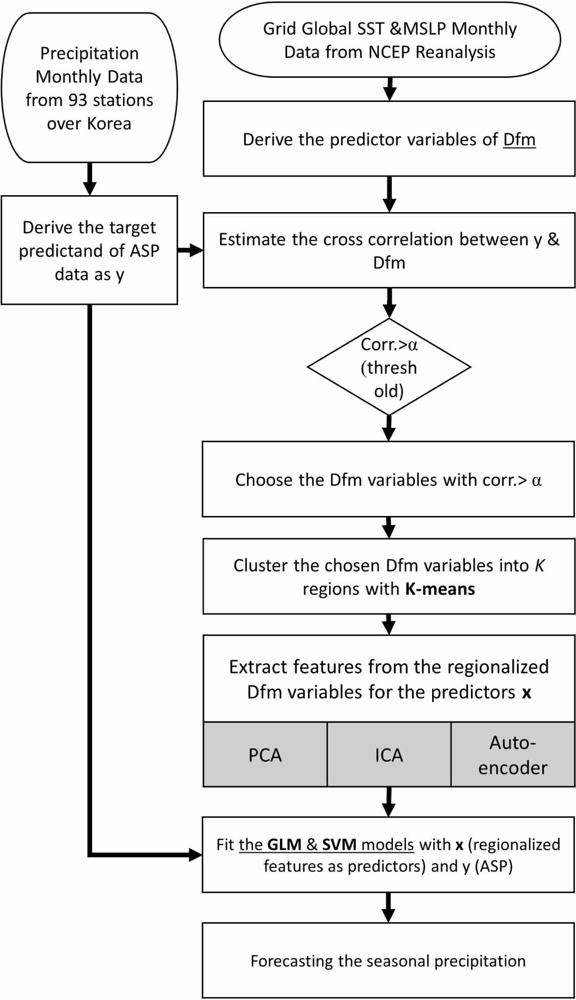
4. Overall procedure and application methodology
The overall procedure in regionalizing the climate variables and forecasting the ASP is graphically presented in figure 1. The regionalization of climate variables (here, SST and MSLP) was at first made by (1) abstracting the gridded climate variables by taking the variables that were higher than a certain threshold of correlation with ASP; (2) clustering the variables over thresholds with the k-means; and (3) extracting feature variables from the clustered variables. In extracting features, three methods as PCA, ICA, and Autoencoder were evaluated, and their results were compared. With the extracted features as predictors, the forecasting of ASP was performed with regression-based models. For Autoencoder, the one hidden node was used, since the only one feature could be extracted from each region. The logsigmoid function and the linear function were applied for encoding and decoding, respectively. One example of the applied autoencoder was presented in figure S2 of the supplementary material.

Figure 1. Schematic description of the ML-based forecasting for the seasonal precipitation (also called ASP in the current study).
Download figure:
Standard image High-resolution imageWith the extracted features for predictors, the GLM and SVM models were applied to forecast the target ASP. The GLM model is a linear model while the SVM model was further tested to check if any performance improvement could be made with more complex models (Chiang and Tsai 2013, Hipni et al 2013, Mokhtarzad et al 2017). For the GLM model, the Gamma distribution was applied, since the employed precipitation data has been known to follow this distribution with a nonnegative domain (Banik et al 2002, Ferraris et al 2003, Hanson and Vogel 2008, Moron et al 2008, Zheng and Katz 2008, Lee 2018). Also, the model performance was checked by applying the K-fold cross validation (KfCV) with the divided dataset as the training and test data sets and K = 4 was used for KfCV. When K = 4, the data is divided by 80% for training and 20% for testing at each fold and this setup has been commonly applied in ML applications (Lee et al 2021). For forecasting ASP, the one-season lag was applied. For example, climate variables of winter season were applied to forecast the spring ASP. The performance of forecasting results was measured with RMSE (root mean square error), MAE (mean absolute error), and R2 defined as:


where  and
and  are the observed and estimated values with n record length and
  represents the mean of observations.
5. ML-based regionalization of climate variables
5.1. Correlation analysis and k-means clustering
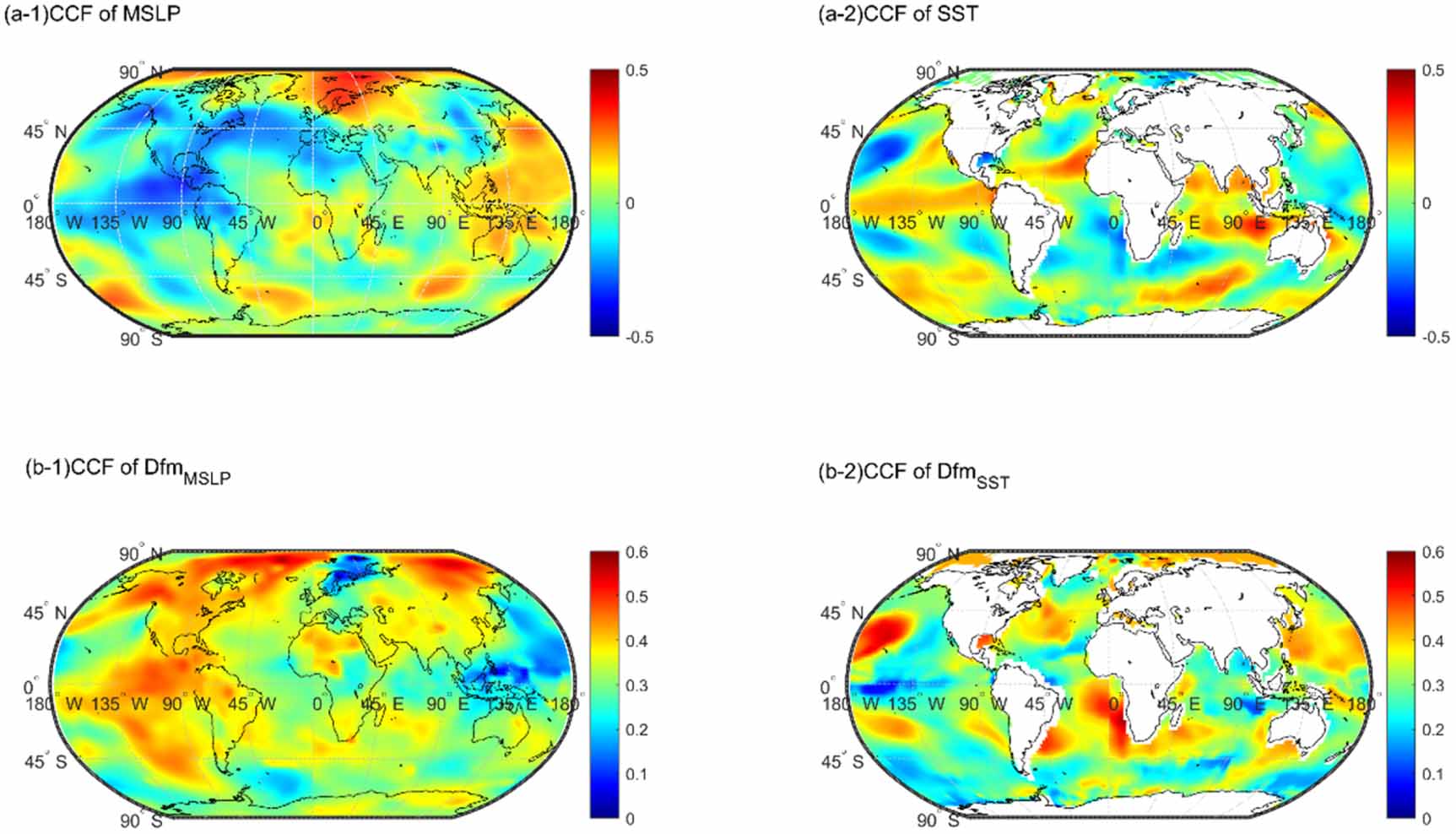
The extracted Dfm variables of MSLP and SST were regionalized to represent the climate characteristics by teleconnecting the ASP of South Korea. K-means clustering was applied, and feature extraction was performed with PCA, ICA, and Autoencoder. For regionalizing climate variables that were teleconnected with the ASP of South Korea, the Dfm SST and MSLP variables must be preselected. In order to perform this, the correlations of the original and Dfm variables with the ASP were checked, as shown in top panels and bottom panels of figure 2, respectively, for the spring season. Note that the presented correlation for the Dfm variables in the bottom panels indicate the largest variables at each grid cell among all the combined variables with the cell.

Figure 2. Correlations between the ASP of the spring season and the climate variables as MSLP (left panels) and the SST variables for the original (top panels (a-1) and (a-2)) and their Dfm variables (bottom panels, (b-1) and (b-2)). See equation (9) for the definition of Dfm and figure 3 for detailed description.
Download figure:
Standard image High-resolution imageThe correlation map with the original MSLP variable in figure 2(a-1) shows high positive correlation in Arctic Ocean and high negative correlation in the east Pacific near the equator region while the SST variable presents high negative correlation in the middle Pacific and high positive correlation around the Indian Ocean near the equator (see figure 2(a-2)). The Dfm MSLP variable in figure 2(b-1) presents much wider region with high positive correlation, especially in the Arctic region between 70° N and 90° N. Also, the SST presents the very high correlation in the middle Pacific (10–25° N and 135–180° W) as shown in figure 2(b-2) and the west side of South Africa.
The correlation results of other seasons are presented in figures S3–S5 for winter, summer, and fall, respectively. Strongly high correlation of the MSLP with the ASP in winter can be observed over the Gulf of Mexico (see figure S3(a-1)). The Dfm variables of the MSLP in summer presents the very strong correlation globally, especially over the north side of North America (figure S4(b-1)). This wide spatial variation can be used to forecast the target ASP. Also, the Dfm of the SST presents some high correlation with the ASP in fall all over the southern ocean areas and North and South Atlantic Ocean (figure S5(b-2)). Those critical zones contain a potential feature structure to forecast the ASP by appropriately zoning the climate variables.
Overall, the correlation analysis indicates that some hot spots exist for each climate variable containing high correlation with the ASP. Therefore, it would be wise to employ the regional effect in forecasting the ASP instead of selecting only a few variables. Once again, the current study was focused on regionalizing the climate variables with high correlation to the target ASP data, as shown in figure 1.
For regionalization of the climate variables with high correlation, we applied different thresholds for correlation and presented the results with the thresholds of [0.53, 0.53, 0.6, and 0.5] for SST and [0.53, 0.54, 0.6, and 0.5] for MSLP in each season of [winter, spring, summer, and fall]. Different thresholds were tested but no better results than those were found (data not shown). With those thresholds, the locations of the selected variables are shown in figures 3 and 4 for the Dfm, SST and MSLP variables in spring. Since the Dfm variables are estimated with the difference of two locations, two different symbols as circle and triangle were employed for the pair locations. Also, the results of the other seasons were presented in the supplementary material of figures S6–S11.

Figure 3. Locations of the variables whose correlations between the Dfm SST variable and the ASP in the spring season are higher than the threshold. Note that (1) each color indicates a group that is differently clustered with the k-means model; and (2) each color has two shapes of circle and triangle representing the locations of a pair of two variables ( and
and  in equation (9)). For example, there are blue circles and blue triangles in panel (a) in the middle of the Pacific and in the middle of the Atlantic, respectively. It presents that blue circles are
  and blue triangles are
  to derive their difference
  variable from equation (9).
Download figure:
Standard image High-resolution image
Figure 4. Locations of the variables whose correlations between the Dfm MSLP variable and the ASP in the spring season are higher than the threshold. See figure 3 for the detailed description of symbols and colors.
Download figure:
Standard image High-resolution imageThe selected variables of the SST for spring in figure 3 are zoned in the middle of the Pacific Ocean and the left side of South Africa as well as some parts in the southwestern Indian Ocean. In contrast, the selected variables of the MSLP for spring (figure 4) are zoned around Arctic Ocean and over Greenland. Note that the northern wind prevails over South Korea during the winter season. It is reasonable that outcoming moisture to South Korea can be affected by the MSLP pattern.
For regionalizing the selected variables over thresholds, the k-means model was applied with different k groups (k= 2,...,9). For example, the results of three groups (i.e. k= 3) for the spring MSLP variable are presented in figure 3(a) and their centroids are also illustrated in figure 5(b). With k= 3, it seems that the variables around west Malaysia and northern Australia are grouped together, as shown in figure 5(b), when those variables should be separated into different groups (figure 3(a)). This indicated that the number of groups (k) for the k-means model was not large enough. Conversely, for k = 8, the variables in the same zone like the center of the Pacific Ocean in figure 5 was split into different groups. The centroids of these variables shown in figure 5(g) were split into four groups as green, blue, yellow, and black triangles. Their corresponding variables presented with circles were in the middle of the Atlantic Ocean for green and in southwestern Malaysia for all the other three groups as blue, yellow, and black.

Figure 5. Locations of the k-means centroids with different k values from k = 2,...,9 for the preselected SST variables in the spring season. Note that (1) each color indicates a centroid that represents the center of each group that is differently clustered with the k-means model; and (2) each color has two shapes of circle and triangle representing a pair of each Dfm variable (see equation (9) and further details in figure 3).
Download figure:
Standard image High-resolution imageA similar behavior was also observed in the MSLP variable in figure 6. Like in figure 6(g) for k= 8, the variables in the same zones, such as northeastern Greenland (0°–90° E and >75° N), were split into seven groups. Especially the group of light blue, yellow, and reds must be categorized into the same group. This indicated that the number of groups was too large and the appropriate number of groups (i.e. k) should be articulated. In this application, we selected the number of groups with substantial proximity by estimating all the distances between centroids as in figure 7 to illustrate how the distances between centroids vary with k. There must be some proximity to each group indicated by the centroids. The proximity of centroids should not be too small to each other, since it indicates that the group is oversplit into groups. Mostly, the minimum distance of the centroids presents some proximity in a small number of k. The number of groups was selected when the minimum distance dropped and stayed afterwards. Since too small a number of groups does not contain enough number of features to model for forecasting, the number of groups (k) was selected as extracting at least four features.

Figure 6. Locations of the k-means centroids with different k values from k = 2,...,9 for the preselected MSLP variables in the spring season. See figures 5 and 3 for a detailed description of symbols and colors.
Download figure:
Standard image High-resolution image
Figure 7. Minimum distances of k-centroids for the selected variables of the SST (left panels) and MSLP (right panels) variables in each season (i.e. (a) winter, (b) spring, (c) summer, and (d) fall) and separated with k-means.
Download figure:
Standard image High-resolution imageIn the left panels of figure 8, the time series of the SST selected variables of five groups in spring are presented. The five groups were sorted with the order that contain a higher number of variables and the first group in figure 8(a) shows the highest number of variables among five groups and the last fourth and fifth groups show the fewest number of variables. In each group, the time series of the selected variables were very similar to each other. This indicates that the separation with the k-means model appropriately clustered the variables.

Figure 8. Time series of the preselected SST variables (left panels) for the spring season and the extracted features (right panels) for four separated regions at each row panels (a)–(d) by three methods as PCA, ICA and Autoencoder. Note that (1) the variables whose correlations between the SST variables are selected in advance and were divided with k-means; and (2) the features were standardized for illustration by subtracting the mean and dividing the standard deviation since each feature has a different range.
Download figure:
Standard image High-resolution image5.2. Feature selection
With these grouped variables with the k-means model, the features were extracted with extraction models as PCA, ICA, and Autoencoder, since each group of the variables contains similar information to each other, rather than individual application of the grouped variables possibly producing model problems as overfitting and multicollinearity. Furthermore, the regional characteristics in grouped variables can be better adopted especially for forecasting the ASP.
Among the extracted features, it is possible that the features are correlated with each other, and highly correlated features might not include new information and produce multicollinearity. Therefore, the correlation matrix was made with the features. In figure 9, the scatterplot and correlation at each pair of the extracted features from PCA were presented with the spring SST Dfm variables as well as their histograms. Among five features, the last two features were highly correlated with each other (correlation: r = 0.98). Note that the features were sorted as the order of higher number of the Dfm climate variables over threshold in each region. This indicates that the last two variables had a smaller number of variables. It is concluded that the features with the lower number might be remnants of the majority of regionalized characteristics with the ASP. Therefore, the first three features were employed for forecasting the ASP in the current study. Further analysis was made by adding more than three features and presented no substantial improvement that could be found by adding more than three features.

Figure 9. Correlation matrix of the selected variables with the feature extraction method of PCA.
Download figure:
Standard image High-resolution imageThe scatterplot between the ASP data in spring and the extracted three features from the SST and MSLP variables are presented in figures 10 and 11, respectively. Also, the other seasons of the SST are shown in figures S12–S14 of the supplementary material. The result presented that the extracted features had certain association with the ASP. The three features extracted from the spring SST variables with the PCA illustrated strong positive correlations with the ASP data (see the left panels of figure 10). Some negative correlation was also observed in the first feature of the Autoencoder (figure 10(a-3)) as well as the second and third features from the ICA.

Figure 10. Scatterplot between the ASP and the extracted three features ((a), (b) and (c) panels) of the Dfm SST variable with PCA (1, left panels), ICA (2, middle panels), and Autoencoder (3, right panels) for the spring season.
Download figure:
Standard image High-resolution image
Figure 11. Scatterplot between the ASP and the three extracted features ((a), (b) and (c) panels) of the Dfm MSLP variables with PCA (1, left panels), ICA (2, middle panels), and Autoencoder (3, right panels) for the spring season.
Download figure:
Standard image High-resolution imageIn addition, the nonlinear relation of features with the ASP can be seen especially in the features from the MSLP variable shown in figure 11. For example, the second and third features extracted with the Autoencoder in figures 11(a-3) and (b-3) showed positive correlation up to 0.7 of the feature and negative correlation higher than 0.7 of the feature value. The correlation and mutual information (MI)-based correlation were measured between the extracted features and the ASP data and their result is presented in tables 1 and 2. Note that the MI-based correlation was estimated as the measurement of nonlinear association by ![$\lambda = \sqrt {1 - {\text{exp}}[ - 2I} ]$](https://content.cld.iop.org/journals/2632-2153/5/1/015019/revision1/mlstad1d04ieqn33.gif) and I is the MI and the MI-based correlation ranged from 0 to 1 (Khan et al
2006). The correlation between the extracted features with the PCA and the ASP in table 1 was between 0.5 and 0.65 for both SST and MSLP variables and similar correlation was presented in the features from the Autoencoder, while the feature from the ICA often presented very low correlation. Meantime, the MI-based correlation in table 2 presents a higher value than the correlation in table 1, indicating the possibility of nonlinear relation. Therefore, a forecasting model that captured the nonlinear relation was applied as the SVM as well as the linear model as the GLM.
and I is the MI and the MI-based correlation ranged from 0 to 1 (Khan et al
2006). The correlation between the extracted features with the PCA and the ASP in table 1 was between 0.5 and 0.65 for both SST and MSLP variables and similar correlation was presented in the features from the Autoencoder, while the feature from the ICA often presented very low correlation. Meantime, the MI-based correlation in table 2 presents a higher value than the correlation in table 1, indicating the possibility of nonlinear relation. Therefore, a forecasting model that captured the nonlinear relation was applied as the SVM as well as the linear model as the GLM.
Table 1. Correlations between the ASP at each season and the extracted features by PCA, ICA, and Autoencoder of the SST and MSLP variables. Note that the features are ordered with higher number of climate variables preselected with higher correlation than a threshold.
| SST | MSLP | ||||||
|---|---|---|---|---|---|---|---|
| Features | PCA | ICA | Autoencoder | PCA | ICA | Autoencoder | |
| Winter | 1 | 0.57 | −0.57 | 0.56 | 0.57 | −0.57 | −0.45 |
| 2 | 0.57 | −0.05 | 0.57 | 0.54 | 0.28 | 0.56 | |
| 3 | 0.56 | 0.56 | −0.53 | 0.55 | 0.44 | 0.60 | |
| Spring | 1 | 0.58 | 0.58 | −0.59 | 0.55 | 0.26 | −0.55 |
| 2 | 0.55 | −0.02 | 0.54 | 0.57 | −0.57 | 0.57 | |
| 3 | 0.54 | −0.01 | 0.51 | 0.56 | 0.16 | 0.56 | |
| Summer | 1 | 0.64 | 0.62 | 0.52 | 0.65 | −0.65 | 0.64 |
| 2 | 0.61 | −0.06 | −0.49 | 0.61 | −0.44 | 0.61 | |
| 3 | 0.61 | 0.18 | 0.67 | 0.64 | −0.38 | −0.60 | |
| Fall | 1 | 0.55 | 0.17 | −0.53 | 0.51 | 0.37 | −0.48 |
| 2 | 0.52 | 0.36 | 0.55 | 0.52 | 0.20 | 0.54 | |
| 3 | 0.52 | −0.52 | 0.55 | 0.51 | −0.05 | 0.52 | |
Table 2. Mutual information (MI)-based correlation between the ASP in each season and the features extracted by PCA, ICA, and Autoencoder of the SST and MSLP variables.
| SST | MSLP | ||||||
|---|---|---|---|---|---|---|---|
| Features | PCA | ICA | Autoencoder | PCA | ICA | Autoencoder | |
| Winter | 1 | 0.68 | 0.68 | 0.66 | 0.68 | 0.69 | 0.61 |
| 2 | 0.67 | 0.46 | 0.66 | 0.67 | 0.44 | 0.69 | |
| 3 | 0.64 | 0.64 | 0.62 | 0.63 | 0.59 | 0.67 | |
| Spring | 1 | 0.74 | 0.73 | 0.72 | 0.66 | 0.56 | 0.66 |
| 2 | 0.67 | 0.49 | 0.64 | 0.67 | 0.67 | 0.66 | |
| 3 | 0.66 | 0.48 | 0.64 | 0.67 | 0.42 | 0.67 | |
| Summer | 1 | 0.70 | 0.70 | 0.60 | 0.74 | 0.74 | 0.70 |
| 2 | 0.72 | 0.54 | 0.67 | 0.74 | 0.60 | 0.74 | |
| 3 | 0.74 | 0.47 | 0.73 | 0.75 | 0.58 | 0.70 | |
| Fall | 1 | 0.65 | 0.49 | 0.63 | 0.60 | 0.52 | 0.55 |
| 2 | 0.63 | 0.55 | 0.63 | 0.64 | 0.41 | 0.65 | |
| 3 | 0.67 | 0.67 | 0.67 | 0.65 | 0.48 | 0.67 | |
6. Forecasting results
The GLM and SVM were employed to forecast the ASP data for water resources management with the extracted features from PCA, ICA, and Autoencoder as predictors. The observed ASP and forecasted ASP with the GLM are shown in figure 12 and a scatterplot in figure 13. The result with the SVM is presented in figures 14 and 15. The winter ASP was fairly forecasted with the GLM as the predictors of the extracted features from the SST predictor shown in figure 12(a-1) except that the largest ASP in 1990 was underestimated from all three extraction methods of PCA, ICA and Autoencoder. Meanwhile, the forecasted value with the extracted features from the Autoencoder highly overestimated this largest value in 1990 as well as in 2019 shown in figure 12(a-2). This overestimation is also presented well in the scatterplot in figure 13(a-2).

Figure 12. Time series of the observed and the forecasted ASP (mm) from the GLM in four seasons ((a), (b), (c), (d) panels) with the extracted features from the SST (1, left panels) and MSLP (2, right panels) variables using PCA, ICA, and Autoencoder. Note that the forecasted data presented in this figure is the result of the KfCV with K = 4.
Download figure:
Standard image High-resolution image
Figure 13. Scatterplot of the observed and forecasted ASP (mm) from the GLM in four seasons ((a), (b), (c), (d) panels) with the extracted features from the SST (1, left panels) and MSLP (2, right panels) variables using PCA, ICA, and AutoEncoder. Note that the diagonal thin line indicates 1–1 line.
Download figure:
Standard image High-resolution image
Figure 14. Time series of the observed and the forecasted ASP (mm) from the SVM model at four seasons ((a), (b), (c), (d) panels) with the extracted features from the SST (1, left panels) and MSLP (2, right panels) variables using PCA, ICA, and AutoEncoder. Note that the forecasted data presented in this figure is the result of the KfCV with K = 4 (i.e. 33-year record was fitted to the SVM model and the rest 10-year data was applied to test, repeating this procedure four times to obtain the 40-year forecasted ASP data).
Download figure:
Standard image High-resolution image
Figure 15. Scatterplot of the observed and forecasted ASP (mm) from the SVM in four seasons ((a), (b), (c), (d) panels) with the extracted features from the SST (1, left panels) and MSLP (2, right panels) variables using PCA, ICA, and AutoEncoder.
Download figure:
Standard image High-resolution imageThis plot of Figure 13(a-2) illustrates that the Autoencoder overestimated some values of the ASP (see the red reverse triangles that were placed above the 1–1 line) and the PCA also overestimated these values but with less magnitude. This large overestimation led to worse performance of the GLM, as presented in table 3. The R2 of the winter ASP with the extracted features of the MSLP variables from the PCA and Autoencoder were 0.33 but the R2 of the ICA was 0.45, which was the best model performance for the winter ASP with the GLM. Meanwhile, the SVM presented the best performance with the features from the Autoencoder with 0.43 of R2, slightly less than the GLM. The nonlinear model, the SVM, might preserve better the characteristics extracted from the Autoencoder.
Table 3. Performance measurements of the GLM forecasted results for the ASP of four seasons with the features extracted by PCA, ICA, and Autoencoder models from the preselected SST and MSLP variables. Note that the the best perfomance model for each season is presented as bold marks.
| SST | MSLP | ||||||
|---|---|---|---|---|---|---|---|
| Season | PCA | ICA | Autoencoder | PCA | ICA | Autoencoder | |
| RMSE | Winter | 30 | 31 | 30 | 28 | 26 | 44 |
| Spring | 53 | 57 | 51 | 46 | 47 | 46 | |
| Summer | 104 | 112 | 117 | 95 | 108 | 99 | |
| Fall | 63 | 71 | 60 | 66 | 76 | 73 | |
| MAE | Winter | 38 | 41 | 38 | 39 | 31 | 87 |
| Spring | 70 | 79 | 63 | 65 | 62 | 65 | |
| Summer | 126 | 136 | 149 | 123 | 144 | 128 | |
| Fall | 80 | 89 | 78 | 83 | 95 | 89 | |
| R2 | Winter | 0.20 | 0.15 | 0.20 | 0.33 | 0.45 | 0.33 |
| Spring | 0.15 | 0.11 | 0.23 | 0.16 | 0.23 | 0.15 | |
| Summer | 0.43 | 0.33 | 0.32 | 0.46 | 0.29 | 0.42 | |
| Fall | 0.35 | 0.23 | 0.37 | 0.29 | 0.06 | 0.26 | |
The spring ASP was often underestimated with the features both from the SST (left panels) and MSLP (right panels) by the GLM and SVM forecasting models in figures 12 and 14, respectively, except that the spring ASP in 1983 was overestimated with the features of the SST extracted from all three methods. The other extreme ASP values such as low values of 2000 and 2001 and high values of 2003 and 2019 were underestimated with all three extraction algorithms for both SST and MSLP variables by the GLM (figures 12(b-1) and (b-2)) and the SVM (figures 14(b-1) and (b-2)). This underestimation is illustrated well especially in figure 15(b-2). In this plot, the corresponding forecasting values of the observed values between 300 and 400 were placed between 200 and 300 for all three extraction algorithms.
This underestimation behavior of the models led to the worst performance of the spring season among all four seasons. The R2 for all three extraction algorithms and the GLM and SVM models did not exceed 0.3, as shown in tables 3 and 4. Note that the target variable was the seasonal precipitation (ASP), and this seasonal precipitation is very difficult to forecast in nature. Even though the performance measurement R2 was less than 0.3, its equivalent correlation was over 0.5 and it was still useful to apply as long as the ASP forecasting. The best performance for the spring ASP was either with the features of the SST from the Autoencoder or with the features of the MSLP from the ICA with 0.28 of R2 with the SVM forecasting model (table 4).
Table 4. Performance measurements of the SVM forecasted results for the ASP of four seasons with the features extracted by PCA, ICA, and Autoencoder models from the preselected SST and MSLP variables. Note that the the best perfomance model for each season is presented as bold marks.
| SST | MSLP | ||||||
|---|---|---|---|---|---|---|---|
| Season | PCA | ICA | Autoencoder | PCA | ICA | Autoencoder | |
| RMSE | Winter | 28 | 29 | 29 | 28 | 31 | 26 |
| Spring | 48 | 52 | 48 | 44 | 45 | 46 | |
| Summer | 103 | 109 | 110 | 92 | 108 | 99 | |
| Fall | 70 | 76 | 67 | 67 | 75 | 67 | |
| MAE | Winter | 36 | 37 | 36 | 35 | 36 | 32 |
| Spring | 60 | 63 | 59 | 61 | 58 | 63 | |
| Summer | 126 | 132 | 135 | 123 | 141 | 131 | |
| Fall | 84 | 91 | 83 | 84 | 94 | 84 | |
| R2 | Winter | 0.26 | 0.23 | 0.26 | 0.33 | 0.29 | 0.43 |
| Spring | 0.26 | 0.19 | 0.28 | 0.23 | 0.28 | 0.19 | |
| Summer | 0.41 | 0.36 | 0.35 | 0.45 | 0.30 | 0.38 | |
| Fall | 0.27 | 0.16 | 0.29 | 0.27 | 0.08 | 0.28 | |
In summer, the forecasting presents the best performance with high association of the extracted features as predictors of the ASP up to 0.65 of correlation and 0.75 of MI-based correlation, as shown in tables 1 and 2. Among others, the PCA features of the MSLP showed the best performance as R2 of 0.46 and 0.45 for both GLM and SVM, respectively. This good performance is presented well in the panels (c-2) of figures 13 and 15 for GLM and SVM, respectively. For the SST variable, the high observed value was overestimated with the Autoencoder features with the GLM model (see the panel (c-1)) of figures 12 and 13.
For the fall season, the Autoencoder features from the SST variables were superior to other variables as 0.37 of R2 with the GLM model, while the SVM model reached only up to 0.29 with the same features from the same climate variables (i.e. SST). This high performance came from the good estimate of the high value in 1985. The RMSE and MAE presented similar results to R2 with only a few differences. Like the GLM in spring, the RMSE showed PCA, ICA, and Autoencoder with the MSLP variable presented similar performances to each other but better than with the SST variable. Also, RMSE and MAE presented different superiority levels with the SVM in spring in that RMSE presented the best performance with the PCA with the MSLP variable, while the MAE showed the best performance for PCA with the SST variable. The RMSE and MAE of the other seasons presented the same superiority as R2. Results indicated that the spring season should be carefully modeled, while the model selection was apparent in other seasons.
The distributional behavior of the predicted values was checked with Kolomogrov–Smiornov test (KS test) (Kottegoda and Rosso 2008). The KS test is a nonparametric test to evaluate whether the maximum difference of two empirical distribution functions (here, observation and predicted values) is within a significance level. When the p-value is smaller than the significance level (e.g. less than 0.1 or 0.05), its null hypothesis that two dataset values are from the same continuous distribution is rejected. The estimated p-value is presented in table 5. Results showed that most of the p-values are in the significance level of 0.05 and 0.1 except a few cases in ICA and Autoencoder. The p-value with the ICA extraction algorithm for the fall SST is less than the significance level of 0.1 for the predicted value with both GLM and SVM models. Also, the p-value for the values predicted with the SVM model has less than the level of 0.1 for both winter SST and MSLP cases. Results indicated that the observed distribution was fairly reproduced with of the predicted values using PCA compared to the other extraction method. The overall KS test indicated that the distribution of the predicted values often matched the observations.
Table 5. Kolmogorov–Smirnov test (i.e. p-value of KS test) with the observed and forecasted series for the ASP of four seasons with the features extracted by PCA, ICA, and Autoencoder models from the preselected Dfm SST and MSLP variables. Note that the p-values lower than 0.1 are presented as bold marks.
| Regression | SST | MSLP | |||||
|---|---|---|---|---|---|---|---|
| Season | PCA | ICA | Autoen | PCA | ICA | Autoen | |
| GLM | Winter | 0.36 | 0.36 | 0.14 | 0.36 | 0.36 | 0.23 |
| Spring | 0.36 | 0.23 | 0.53 | 0.53 | 0.53 | 0.14 | |
| Summer | 0.53 | 0.53 | 0.36 | 0.89 | 0.53 | 0.89 | |
| Fall | 0.53 | 0.08 | 0.36 | 0.36 | 0.36 | 0.36 | |
| SVM | Winter | 0.23 | 0.36 | 0.04 | 0.23 | 0.23 | 0.08 |
| Spring | 0.89 | 0.23 | 0.14 | 0.53 | 0.89 | 0.14 | |
| Summer | 0.72 | 0.89 | 0.23 | 0.89 | 0.72 | 0.23 | |
| Fall | 0.72 | 0.02 | 0.23 | 0.36 | 0.36 | 0.14 | |
The minimum statistics of predicted and observed seasonal precipitation were compared, as shown in figure 16, since the major application of seasonal forecasting in the current study is water resources management, especially in an extreme condition like drought. With the GLM model (figure 16), the minimum statistics were underestimated in all seasons and by all the extracted methods of the MSLP and SST variables. The statistics with the SVM model were better preserved, even though they were underestimated in spring with all the extraction methods and the variables used but still their magnitudes were less underestimated with the SVM than the one of the GLM.

Figure 16. Minimum statistics of the observed and forecasted ASP (mm) from the GLM (panel (a)) and SVM (panel (b)) in four seasons using PCA (◇), ICA (x25CB;), and Autoencoder (∇).
Download figure:
Standard image High-resolution image
7. Summary and conclusions
Seasonal precipitation forecasting is essential for water resources management, including drought mitigation. However, seasonal precipitation has been known to be difficult to forecast due to its uncertainty nature and effect from highly complex climate systems, and only a few successful forecasting models can be found. Meanwhile, a number of globally gridded climate variables have been produced but their application to seasonal forecasting has not been much successful. Therefore, the current study proposed a novel procedure employing the entire globally gridded climate variables by regionalizing the highly correlated climate variables with the target ASP using the k-means clustering; extracting the features with the ML-based models as PCA, ICA, and Autoencoder; and finally regressing the extracted features with the linear model of GLM and the nonlinear model of SVM.
The result indicated that the k-means clustering appropriately regionalized the highly associated climate variables of the SST and MSLP for all seasons. The extraction algorithms performed reasonably well in different seasons and climate variables. The PCA extracted well the features from the climate variables and the extracted features from the PCA performed the best in summer with the MSLP and in fall with the SST especially combined with the linear model of GLM. The Autoencoder presented its superiority in winter with the MSLP and in spring with the SST especially combined with the nonlinear SVM model. The ICA extraction algorithm sometimes showed good performance in winter and spring with the MSLP combined with the GLM model.
Overall, results concluded that the proposed procedure was a good alternative in forecasting the seasonal precipitation of ASP for water resources management by regionalizing the highly associated climate variables as hot spots, extracting the critical features, and regressing the ASP with the extracted features. Further analysis was made by combining the features from different extraction algorithms of PCA, ICA, and Autoencoder and combining the features from the MSLP and SST variables. The result was not successful by producing no better results than the individual variables and the features from each extraction algorithm. In the current study, application was only made for forecasting the ASP over South Korea. However, the proposed procedure can be easily adopted to another region and for forecasting other hydrological and environmental variables.
Acknowledgments
The authors acknowledge that this research was partially supported by a Grant (2022-MOIS63-001) from Cooperative Research Method and Safety Management Technology in National Disaster funded by the Ministry of Interior and Safety (MOIS, Korea). This work was also supported by the National Research Foundation of Korea (NRF) Grant funded by the Korean Government (MSIT) (2023R1A2C1003850).
Data availability statement
All data that support the findings of this study are included within the article (and any supplementary files).
Conflict of interest
No potential conflict of interest was reported by the author(s).
Supplementary data (6.1 MB DOCX)