The effects of topological features on convolutional neural networks—an explanatory analysis via Grad-CAM

Images consist of discrete pixels (or voxels) on a fixed uniform grid in Euclidean space $\mathbb{R}^d$. Intuitively, these pixels have some kind of connection structure. This connection structure may form an edge or a surface of image. With the aid of computational topology, this connectivity can be handled suitably and calculated numerically.

Graphs or simplicial complexes are typical examples, which represent the connection between objects such as edges or planes. Cubical complexes are generally used to represent the connectivity in images. Since images are defined on mesh, cubical complexes, whose bases are elementary cubes, are suitable to represent the topological features of the given image data.

A cubical complex is a collection of vertices, edges, squares, and higher dimensional analogues on a regular grid in $\mathbb{R}^d$. The formal definition is as follows:

Definition 1 (Cubical complex). An elementary cube $Q \subset \mathbb{R}^d$ is defined as a product $Q = I_1 \times \cdots \times I_d$ where each I_j is either a singleton set $\left\{m\right\}$ or a unit-length interval $[m,m+1]$ for some integers $m\in \mathbb{Z}$. The number k of the unit-length intervals in the product of Q is called the dimension of cube Q and we call Q a k-cube. If Q and Qʹare two cubes and $Q\subseteq Q^{^{\prime}}$, then Q is said to be a face of Qʹ. A cubical complex X in $\mathbb{R}^d$ is a collection of k-cubes ($0\leqslant k \leqslant d$) such that

• (i)  
  every face of a cube in X is also in X;
• (ii)  
  the intersection of any two cubes of X is either empty or a face of each of them.

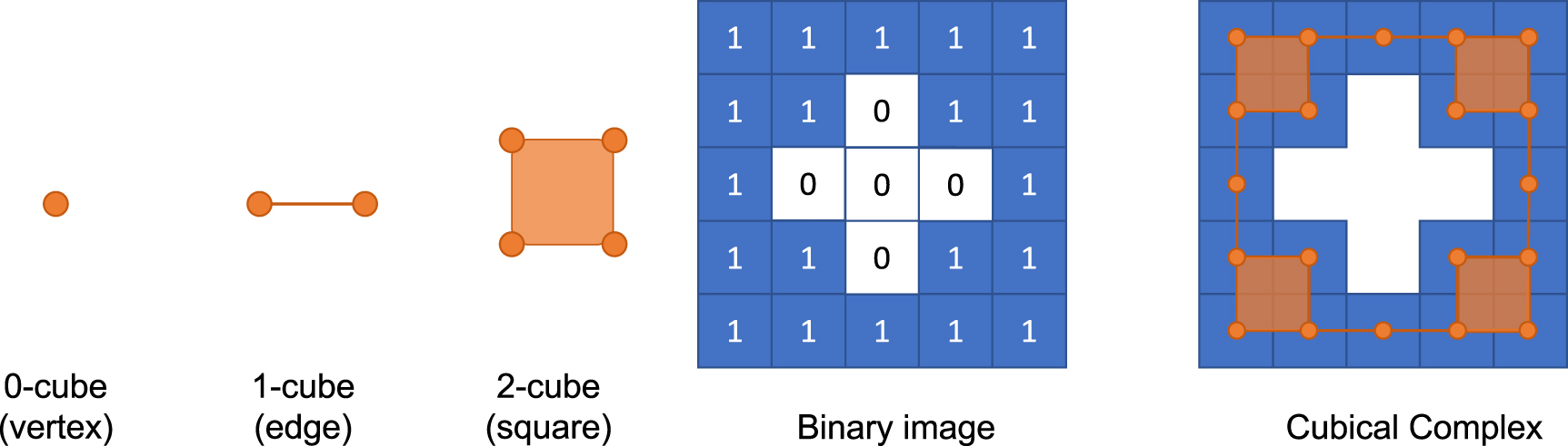
In order to obtain a cubical complex of a given image, choose an appropriate threshold (grayscale value) and obtain a binary image. Those pixels (e.g. figure 1) assigned the value of 1 in the binary image on the grid in $\mathbb{R}^2$ are regarded as a point (vertex). Now one can define a cubical complex on the point set. See figure 1.

Zoom In Zoom Out Reset image size

Representing an image as a cubical complex allows us to observe the topological features in the image such as the connected components and loop structures. Moreover, these topological features in the image are characterized by the notion of homology. Hence, one may find the number of connected components or loops in the image by calculating its homology. Homology of an image is obtained through the following steps.

• (i)  
  Choose a threshold and define a cubical complex X.
• (ii)  
  For each $k = 0,1,2$, define a free abelian group (or vector space over finite field $\mathbb{F}_2$) $C_k(X)$ whose basis is a set of all k-cubes in X. Each $C_k(X)$ is called kth chain group or chain module. Let $C_{-1}(X) = 0$.
• (iii)  
  For each k, define a homomorphism $\partial_k : C_k(X) \rightarrow C_{k-1}(X)$ which maps k-cubes to sum of its faces in $C_{k-1}(X)$. Each $\partial_k$ is called the kth boundary operator.
• (iv)  
  Now, the kth homology group $H_k(X)$ is defined as the quotient space $\ker{\partial_k}/\textrm{im}\partial_{k+1}$ for each k.

Notice that the composition $\partial_{k} \circ \partial_{k+1}$ is equivalent to the zero map. It follows $\textrm{im}\partial_{k+1}\subseteq\ker\partial_k$ and then the homology group $H_k(X)$ is well-defined.

The rank of the kth homology group $H_k(X)$ is called the kth Betti number or generator. Roughly speaking, the Betti number is the number of k-dimensional holes in X such as connected components (zero-dimensional holes), loops (one-dimensional holes) and so on.

Using homology, useful topological information can be calculated through matrix computations. For this, we need to select appropriate thresholds to define a cubical complex. Persistent homology, a major tool of TDA, is a generalized concept of homology that helps us to learn how homology changes with increasing thresholds. The topological features used in a CNN-TDA Net considered in this paper are calculated based on persistent homology.

A grayscale image is represented by a function $\mathcal{I} : \Omega\subseteq\mathbb{R}^2 \rightarrow \mathbb{R}$ where Ω is the grid on which the image is defined and $\mathcal{I}(v)$ is the grayscale value of the pixel $v \in \Omega$. In general, the grayscale value of one pixel takes an integer value between 0 and 255. Additionally, let $\mathcal{I}_{-\infty}$ be an empty set. A sublevel set of a grayscale image for a value $0\leqslant i\leqslant 255$ is a set of all pixels in the grid with a pixel intensity less than or equal to i, i.e. $\mathcal{I}_i : = \left\{v \in \Omega : \mathcal{I}(v) \leqslant i\right\}$. A sublevel set may be realized with a binary image in which 1 is assigned to pixels of the sublevel set and 0 is assigned to pixels on the remaining grid. We note here that we mainly consider the grayscale images in this paper and the colored images will be considered in our future research.

Let X_i be the cubical complex defined on the binary image of the sublevel set $\mathcal{I}_i$. Then a sequence $\emptyset = \mathcal{I}_{-\infty} \subseteq \mathcal{I}_{0} \subseteq \cdots \subseteq \mathcal{I}_{255}$ of the sublevel sets induces a nested sequence of cubical complexes $\emptyset = X_{-\infty}\subseteq X_0 \subseteq \cdots \subseteq X_{255} = X$. This sequence is called the filtration.

The inclusion relation of cubical complexes in the filtration is naturally extended to the inclusion relation of the corresponding homology. More precisely, this idea is based on the functoriality that appears throughout various mathematical applications. That is, the inclusion map $\iota_{i,j} : X_i \hookrightarrow X_j\; (i\leqslant j)$ between two cubical complexes $X_i \subseteq X_j$ is extended to the inclusion linear map $f^{\,\,k}_{i,j} : H_k(X_i) \hookrightarrow H_k(X_j)$ between two vector spaces $H_k(X_i)$ and $H_k(X_j)$ for fixed k. For $i_1 \leqslant i_2 \leqslant i_3$, the following holds :

$$\begin{align} f^{\,\,k}_{i_2,i_3} \circ f^{\,\,k}_{i_1,i_2} = f^{\,\,k}_{i_1,i_3} \;\;\;\ \textrm{for all}\ i_1 \leqslant i_2 \leqslant i_3. \end{align} \tag{ 1 }$$

Now we can define the persistent module and homology:

Definition 2 (The k th persistence module). For the given filtration $\emptyset = X_{-\infty}\subseteq X_0 \subseteq \cdots \subseteq X_{n} = X$ and fixed dimension k, the kth persistent module PM_k consists of the pair of the k-dimensional homology groups (or vector spaces) and linear maps

$$\begin{align} PM_k = \left\{\left\{H_k(X_i)\right\}_{i = 1}^n, \left\{f^{\,\,k}_{i,j}\right\}_{1\leqslant i \leqslant j \leqslant n}\right\} \end{align} \tag{ 2 }$$

where $H_k(X_i)$ is the kth homology for each X_i and $f^{\,\,k}_{i,j} : H_k(X_i) \hookrightarrow H_k(X_j)$ are the linear maps induced by the inclusions $\iota_{i,j} :X_i \hookrightarrow X_j$ for all $i \leqslant j$. The kth persistent homology groups $H_k^{i,j}$ are the images of $f_{i,j}$; that is, $H_k^{i,j}: = \textrm{Im}{f_{i,j}}$.

The functoriality of persistent homology plays a critical role to analyze whole scheme for the evolution of the space with respect to the variation of parameters. One can observe overall homology according to the change of the parameter.

Recall that the generators of each homology represent the connectivity of space, such as connected components, loops, voids and so forth. Then for any i and j with $i\leqslant j$, the generator of the previous homology group $H_k(X_i)$ may be maintained as the generator of the latter $H_k(X_j)$ under the linear map $f^{\,\,k}_{i,j}$ or no longer be a generator as expressed by the linear combination of the generators of $H_k(X_j)$. $H_k(X_j)$ may also contain new generators that were not present in $H_k(X_i)$. This means that information about the connectivity of each space is 'newly born', 'persist', or 'merged away' as the scale changes.

The persistent homology $H_k^{i,j}$ summarizes this information. The rank of $H_k^{i,j}$ is called the kth persistence Betti number and denoted by $\beta_k^{i,j}$. $\beta_{k}^{i,j}$ represents the number of the kth homological classes persisting between i and j.

The decomposition theorem of persistence module tells us that persistent homology can be decomposed algorithmically by a multiset of intervals $\left\{[b_n,d_n]\right\}_n$ in which each interval $[b,d]$ corresponds to a topological invariant that is born at b and dies at d [29]. Then, the collection of intervals $\left\{[b_n,d_n]\right\}_n$ for persistent homology is called persistence barcode. The persistence diagram is a collection of points in $\mathbb{R}^2$ that each point $(b_n,d_n)$ corresponds to the interval $[b_n,d_n]$ in barcode. Persistence barcode and persistence diagram have exactly the same information.

Figure 2 shows persistent homology of the left image in (a). (a) shows the filtration of the given image, (b) the corresponding persistence barcode, and (c) the corresponding persistence diagram. For the filtration value i = 0, only five pixels with a zero intensity are activated, and form five connected components. These five connected components correspond to the five solid lines in persistence barcode. For X₁, the five connected components are integrated into one so that the four solid lines in the barcode end at i = 1. One connected component remains until X₄ as shown in the figure—the first orange lines in the barcode and the point $(0, 4)$ in the diagram. For one-dimensional homology, one loop enclosed by the connected components is born at X₁ and dies at X₄ corresponding to the red dashed line in the barcode and the red dot in the diagram.

Zoom In Zoom Out Reset image size

As shown above, persistence diagram contains useful topological characteristics of the given data. However, it cannot be fed into the neural networks directly due to its multiset nature. Vectorization is a way of feeding the topological features appearing in persistence diagram into the neural networks. Various vectorization methods have been proposed that convert persistence diagram into a finite size representation, such as BS, persistence landscape, and PI. Let $\epsilon_1, \epsilon_2, \cdots, \epsilon_d$ be a sequence of filtration values and $k \in \mathbb{N}$ be a fixed number. Briefly speaking, the kth BS [14] is defined by $\left(BC(\epsilon_1), \ldots, BC(\epsilon_d)\right) \in \mathbb{R}^d$ where $BC(\epsilon) = \left|\left\{(b,c)\in PD : \epsilon \in [b,d]\right\}\right|$. The kth persistence landscape [13] is defined by $(\lambda_l(\epsilon_1),\ldots,\lambda_l(\epsilon_d)) \in \mathbb{R}^{d}$ where $\lambda_l(t)$ is the lth largest value of $\max\left(\min(t-b,d-t), 0\right)$. A PI [12] is an image-like representation that applies the Gaussian kernel to each point in persistence diagram.

In this work, we utilized BS for the CNN-TDA Net as the vectorization of topological features. For the given filtered complex X_ε , the BS is constructed by tracking the variation of the Betti numbers of each complex X_ε with the increasing value of ε. In other words, the Betti curve (BC) is a function assigning each ε value to the Betti number $\beta_k(X_\epsilon)$.

Definition 3 (Betti curve/Betti sequence). Let $\epsilon_1\leqslant \epsilon_2 \leqslant \cdots \leqslant \epsilon_n$ be the equally spaced points in the parameter space. For the persistence diagram PD_k for the kth persistence module $PM_k = \{\{H_k(X_i)\}_{i = 1}^n, \{f^{\,\,k}_{i,j}\}_{1\leqslant i \leqslant j \leqslant n}\}$, the kth Betti curve is a function defined by

$$\begin{align} BC_{k} : \mathbb{R} \longrightarrow \mathbb{N}, BC_{k}(\epsilon) = \left| \left\{(b,c)\in PD_{k} : \epsilon \in [b,d]\right\}\right|. \end{align} \tag{ 3 }$$

The kth Betti sequence is the sequence of the numbers

$$\begin{align} \left(BC_{k}(\epsilon_1), \ldots, BC_{k}(\epsilon_n)\right) \in \mathbb{R}^n. \end{align} \tag{ 4 }$$

The BC is easy to compute. One can observe that the BC is the linear combination of the indicator functions $\mathbf{1}_{[\epsilon_i,\epsilon_{i+1}]}$. Thus, the BC is a step function, and its space forms a vector space with L_p -norm $\lVert BC \rVert_p : = \left(\int_{\mathbb{R}} \lvert BC(t)\rvert^p dt \right)^{\frac{1}{p}}$. It follows that the BC is suitable to statistical inference and machine learning [30].

By stacking the kth BSs along the dimensions, we can represent them as a multichannel sequential data structure where each data point is a d-dimensional vector, i.e,

$$\begin{align} \left( \begin{bmatrix} BC_0(\epsilon_i) \\ BC_1(\epsilon_i) \\ \vdots \\ BC_d(\epsilon_i) \end{bmatrix} \right)_{i = 1}^{n}. \end{align} \tag{ 5 }$$

This interpretation of the BSs as sequential data motivated us to utilize a one-dimensional CNN for analyzing BSs.

A CNN-TDA Net (or simply TDA-Net) [17] is a family of neural networks that take an image and the corresponding topological features as inputs to predict its label. TDA-Net consists of three subnetworks: an image network, a TDA network (or a topology network), and a prediction head. An image network f_img is a CNN that takes an image as an input and extracts a fixed-size feature vector. A TDA network f_tda is a parameterized nonlinear function that encodes TDA features corresponding to the input image into a feature vector of a fixed size. That is, for the given image $\mathbf{x}_{\textrm{img}}$ and the corresponding TDA features, $\mathbf{x}_{\textrm{tda}}$, we have

$$\begin{align} f_{\textrm{img}}\left( \mathbf{x}_{\textrm{img}} \right) = \mathbf{h}_{\textrm{img}}, \end{align} \tag{ 6 }$$

$$\begin{align} f_{\textrm{tda}}\left( \mathbf{x}_{\textrm{tda}} \right) = \mathbf{h}_{\textrm{tda}}, \end{align} \tag{ 7 }$$

where $\mathbf{h}_{\textrm{img}}$ and $\mathbf{h}_{\textrm{tda}}$ are the feature vectors with specific dimensions determined by the input size and the network architecture, respectively. Again, examples of topological features could be PI, PL, and BS. The structure of the TDA network depends on the shape of the vectorization. For example, one can use a two-dimensional CNN for PI because PI is given as a two-dimensional image and a one-dimensional CNN for PL and BS because both PL and BS are basically one-dimensional sequences of numbers. In this paper, we focus on the effects of topological features using BS, simply referred to as a CNN-BS Net.

The concatenation of $\mathbf{h}_{\textrm{img}}$ and $\mathbf{h}_{\textrm{tda}}$ is fed into the prediction head. A typical choice for a prediction head f_head is an MLP, but any nonlinear function that produces a prediction can be used:

$$\begin{align} f_{\textrm{head}}\left( \begin{bmatrix} \mathbf{h}_{\textrm{img}} \\ \mathbf{h}_{\textrm{tda}} \end{bmatrix}\right) = \widehat{\mathbf{y}}, \end{align} \tag{ 8 }$$

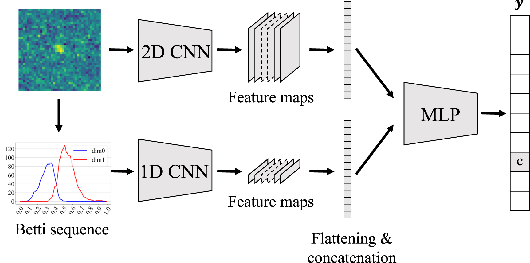
where $\widehat{\mathbf{y}}$ is a scalar for a one-dimensional regression task or a vector for a classification task. Figure 3 shows the schematic structure of a TDA-Net, i.e. a CNN-BS Net. The top-left figure shows the original image. The main image source is located at the image center with a noisy background. The bottom left figure shows the BSs; the blue solid line represents the zero-dimensional BS and the red the one-dimensional BS. The image and the BSs are fed into the TDA-Net in the figure. The image passes through the two-dimensional CNN (denoted as the 2D CNN in the figure) to produce feature maps. The BSs go through the one-dimensional CNN (denoted as the 1D CNN in the figure), producing into feature maps. Both the image and topology feature maps are fed into the MLP towards the prediction head.

Zoom In Zoom Out Reset image size

Grad-CAM [25] is a technique for visually explaining the decision of a CNN-based model. It measures the influence of each pixel in the feature maps of the last convolutional layer on the model prediction. Let y^c be the prediction of the model for a class c and A^k be the kth feature map of the last convolutional layer. Then, the class-discriminative localization map Grad-CAM, which has the form of a heat map, is computed as follows:

$$\begin{align} L_{\textrm{Grad-CAM}}^{c} = \operatorname{ReLU} \left( \sum_k \alpha_k^c A^k \right), \end{align} \tag{ 9 }$$

where $\alpha^{c}_{k}$ is the importance of the kth feature map. $\alpha^{c}_{k}$ is defined as the average of the partial derivative values of y^c with respect to each pixel in A^k :

$$\begin{align} \alpha^{c}_{k} = \frac{1}{Z} \sum_{i, j}\frac{\partial y^c}{\partial A^k_{i, j}}, \end{align} \tag{ 10 }$$

where (i, j) is the coordinate of each pixel in the feature map A^k and Z is the number of pixels in A^k . In (9), $\operatorname{ReLU}(x): = \max(0, x)$ ensures that $L^{c}_{\textrm{Grad-CAM}}$ is greater than or equal to zero. The resolution of $L_{\textrm{Grad-CAM}}^{c}$ is the same as that of the feature maps, which is generally smaller than that of the input image. Thus, $L^{c}_{\textrm{Grad-CAM}}$ is upsampled to $\widetilde{L}^{c}_{\textrm{Grad-CAM}}$ which has the same resolution as the input image by using bilinear interpolation. The visual interpretation of the model is obtained by superimposing $\widetilde{L}^{c}_{\textrm{Grad-CAM}}$ on the input image. Figure 4 shows a schematic illustration of how the heat map is calculated using Grad-CAM applied to the CNN. The figure shows how the gradients of the model prediction with respect to feature maps are integrated through ReLU towards the heat map, which is then displayed on the original image after being upsampled. The area in the warmest color in the bottom-left heat map indicates the main feature that the CNN uses for prediction in the image.

Zoom In Zoom Out Reset image size

To the best of our knowledge, the current work is the first approach to apply Grad-CAM to CNN-TDA Nets and analyze the role of TDA features on a CNN. The application of Grad-CAM to a multimodal network was initially implemented in [31]. Here, we first provide an elaborated formulation. We perform Grad-CAM on the last feature maps A of an image network and the last feature maps B of a TDA network, respectively, i.e.

$$\begin{align} L^c_{\textrm{image}} : = \operatorname{ReLU}\left( \sum_k \alpha_k^c A^k \right), \end{align} \tag{ 11 }$$

$$\begin{align} \alpha_k^{c} = \frac{1}{Z_{A^k}} \sum_{i,j} \frac{\partial y^c}{\partial A^{k}_{ij}}, \end{align} \tag{ 12 }$$

where A^k is the kth feature map of the image network and $Z_{A^k}$ is the total number of pixels in A^k . And

$$\begin{align} L^c_{\textrm{tda}} : = \operatorname{ReLU}\left( \sum_n\beta_n^c B^n \right), \end{align} \tag{ 13 }$$

$$\begin{align} \beta_n^{c} = \frac{1}{Z_{B^n}} \sum_{m} \frac{\partial y^c}{\partial B^{n}_{m}}, \end{align} \tag{ 14 }$$

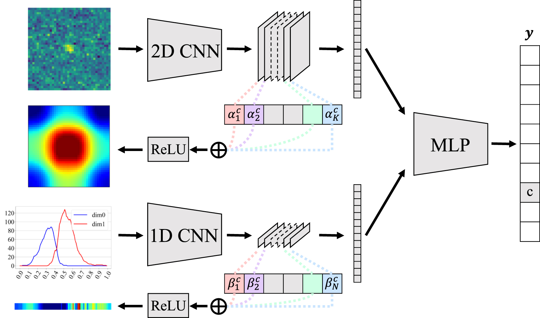
where Bⁿ is the nth feature map of the TDA network in the one-dimensional CNN and $Z_{B^n}$ is the total number of pixels in Bⁿ . Then, $L^c_{\textrm{image}}$ and $L^c_{\textrm{tda}}$ are upsampled to $\widetilde{L}^c_{\textrm{image}}$ and $\widetilde{L}^c_{\textrm{tda}}$ so that they have the same resolution as the input image and the computed BS, respectively. Figure 5 illustrates the procedure of Grad-CAM analysis on the multimodal network. In figure 5, the top-left figure shows the original input image, which has the main image source at the center in a noisy background. The middle left figure shows the heat map obtained by Grad-CAM applied to the image network and displaced on the original image after being upsampled. The bottom left figure shows the zero- and one-dimensional BSs of the original image through the steps of building cubical complexes. The blue solid line represents the zero-dimensional BS and the red solid line the one-dimensional BS, as shown in figure 3. Unlike figure 3, the figure shows the heat map by Grad-CAM applied to the topology network. Figure 5 shows how those heat maps for the image and topology networks are obtained in the CNN-TDA Net. As shown in the figure, the prediction head is a nonlinear function of those two feature maps from the image and topology networks. Thus, the heat map of the image network is obviously affected by the topology network.

Zoom In Zoom Out Reset image size

Here we note that there are no cross-effects of both feature maps in the MLP after the concatenation of the two flattened vectors of A and B. With ReLU activation function, it is guaranteed that there is no nonlinear term between any $A^k_{ij}$ and $B^{n}_{m}$ when y^c is a predicted logit (before applying the Softmax function). Hence, the partial derivative with respect to $A^k_{ij}$ or $B^{n}_{m}$ is either zero or the linear weight corresponding to each of them.

In order to interpret the Grad-CAM results of a TDA network, we define the topological inverse image of a range of filtration values. Let $I \in \mathbb{R}^{h \times w}$ be the grayscale image of the height h and width w, and $t_a \leqslant t_b$ be two filtration values. We define the sublevel image $I^{(-\infty, t_a)} \in \mathbb{R}^{h \times w}$ of I at t_a as follows:

$$\begin{align} I^{(-\infty, t_a)}_{i,j} : = \begin{cases} I_{i,j} \quad \textrm{if}\ I_{i,j} < t_a \\ 0 \quad \textrm{otherwise} \end{cases}\!\!\!\!\!\!, \end{align} \tag{ 15 }$$

for $i = 1, 2, \cdots, h$, and $j = 1, 2, \cdots, w$. Then, the topological inverse image of I of the range $[t_a, t_b)$ is defined as the subtraction of $I^{(-\infty, t_a)}$ from $I^{(-\infty, t_b)}$, i.e.

$$\begin{align} I^{[t_a, t_b)}: = I^{(-\infty, t_b)}-I^{(-\infty, t_a)}. \end{align} \tag{ 16 }$$

That is, $I^{[t_a, t_b)}$ is the image I where the region that has intensities out of the range $[t_a, t_b)$ is set to be zeros. The visual explanation of the inverse image is shown in figure 6. The left figure (a), in figure 6, is the original grayscale image of a point source with noisy background. As shown in the figure, the main object of interest is located in the image center. As the noise intensity in the background is non-negligible compared to the intensity of the main object in the center, CNN could be biased to such high-frequency noise in the background. Figure (b) shows two filtration values t_a and t_b with $t_a \lt t_b$. Figures (c) and (d) show $I^{(-\infty, t_b)}$ and $I^{(-\infty, t_a)}$, respectively, where it is clear that background noise is still significant. Figure (e) shows the topological inverse image, $I^{[t_a, t_b)}$, in the range of $[t_a, t_b)$. As shown in (e), the main image source is more outstanding than in (c) and (d). As shown later, the heat map by Grad-CAM indicates well the main image characteristics through the topological inverse image map.

Zoom In Zoom Out Reset image size

We investigate the topological inverse image of the range near the filtration value that has the maximum in Grad-CAM, that is, the filtration value where the heat map by Grad-CAM has the warmest color. Here, the range is determined by the receptive field of the TDA network. We recall that the receptive field of a pixel in feature maps is the region in the input involved in the calculation of that pixel. Hence, we consider the topological inverse image $I^{[t_a, t_b)}$ such that

$$\begin{align} t_a = t^{*} - \frac{l_{\textrm{rf}}}{2 l_{\textrm{bc}}}, \end{align} \tag{ 17 }$$

and

$$\begin{align} t_b = t^{*} + \frac{l_{\textrm{rf}}}{2 l_{\textrm{bc}}}, \end{align} \tag{ 18 }$$

where $t^{*} = \operatorname*{argmax} \widetilde{L}^{c}_{tda}$, l_rf is the length of the receptive field of the TDA network, and l_bc is the length of the BS. Therefore, the topological inverse image can be interpreted as a transformation from a feature map obtained from the BS and Grad-CAM into the region of the input image. While the inverse of a given BS may not be unique in general, the definition of our topological inverse image ensures that it can always be obtained when an image and two filtration values are given. As shown in the following section, Grad-CAM analysis shows that the topological inverse image identified by the heat map is well-matched with the main image of interest. This implies that the topology network is less sensitive to background noise than the image network. The reproducible codes for the experiments with the HAM1000 dataset can be found at https://github.com/HiddenBeginner/cnntdanet_gradcam.

We consider the grayscale image classification problem; the cubical complex explained in section 2 can be directly applied to grayscale images. We conducted experiments using those two famous image classification datasets, i.e. the transient versus bogus image dataset and the HAM10000 dataset.

5.1.1. Transient-vs-bogus dataset

5.1.2. The HAM10000 dataset

We conducted Grad-CAM analysis on the CNN-BS Net. The architecture of the image network follows that of O'TRAIN [36]. O'TRAIN performs well on various grayscale images, particularly on the transient versus bogus image classification problem, and is widely used in the astrophysical image analysis community. For the topology network, we selected WaveNet [37], which is suitable for sequential data because the BS can also be regarded as sequential data, as explained in section 2.2. Table 1 shows the optimized image network of O'TRAIN architecture (top) and the topology network adopted from the architecture of WaveNet (bottom). Here, we note that all convolutional operations are applied after zero padding. The concatenation of the two flattened feature maps is fed into the classification head. The classification head is an MLP with two hidden layers with 512 and 256 neurons. More training details and learning curves are provided in appendix A.

Table 1. The architecture of O'TRAIN [36] (top) and WaveNet [37] (bottom) before the classification head. (i: the layer number, k: the filter size, $n_{c_i}$: the number of filters, p: the dropout rate, r_dilated: the rate of dilation).

i	Operator	$n_{c_i}$
1	Conv2D $(k = 3)$	16
2	Conv2D $(k = 3)$	32
3	AvgPooling2D $(k = 2)$	32
4	Conv2D $(k = 3)$	64
5	MaxPooling2D $(k = 2)$	64
6	Dropout $(p = 0.3)$	64
7	Conv2D $(k = 3)$	128
8	MaxPooling2D $(k = 2)$	128
9	Dropout $(p = 0.3)$	128
10	Conv2D $(k = 3)$	256
11	MaxPooling2D $(k = 2)$	256
12	Flatten	—

i	Operator	$n_{c_i}$	rdilated
1	Conv1D $(k = 2)$	20	1
2	Conv1D $(k = 2)$	20	2
3	Conv1D $(k = 2)$	20	4
4	Conv1D $(k = 2)$	20	8
5	Conv1D $(k = 2)$	20	1
6	Conv1D $(k = 2)$	20	2
7	Conv1D $(k = 2)$	20	4
8	Conv1D $(k = 2)$	20	8
9	Conv1D $(k = 1)$	10	—
10	Flatten	—	—

Figures 7 and 8 show the Grad-CAM analysis of the transient versus bogus image datasets. Figure 7 shows the results of the multimodal Grad-CAM analysis of the image that contains the transient in the image center. In the figure, (a) is the image that contains a single transient. As shown in the figure, the transient, a round and bright object, is located at the image center. The heat maps, those color images in the top row in columns (b) through (g), are the Grad-CAM heat maps over the single CNN (i.e. without the topology network). The heat maps in the bottom row are the Grad-CAM heat maps over the CNN-BS Net, that is, the heat maps when the topology network is combined with the original CNN. The images in column (b) are the aggregated Grad-CAM heat maps displayed over the input image, (a), with (top) and without (bottom) the topology network, respectively. Those images in column (b) show slight differences between the networks with and without the topology network. The bottom figure in Column (b) shows that the heat map is concentrated around the transient and more symmetric than that of the single CNN shown in the top. Here notice that the images in column (b) are the aggregated images of all the individual feature maps obtained by the network as indicated in (9) and (10). Thus, it is worth investigating how the heat map of each individual feature map changes when combined with the topology network. Those images in columns (c) through (g) are the heat maps of the top five feature maps that have the highest channel importance values defined in (10). As shown in the figure, the heat map of each feature map with the topology network is more centered around the transient than the heat map of the single CNN except for the 5th feature map in Column (g). Although there are differences between the single CNN and CNN-BS Net, the aggregated heat maps in column (b) indicate that both the single CNN and the CNN-BS Net capture the desired transient features reasonably. The image in column (h) is the topological inverse image $I^{[t_a, t_b)}$ where t_a and t_b are defined in (17) and (18) for the length of the receptive field $l_{\textrm{rf}} = 32$, the dimension of the BSs $l_{\textrm{bc}} = 100$, and the filtration value $t^{*}$ that has the maximum in Grad-CAM on the BS shown in column (i). The blue line in the image of (i) is the zero-dimensional BS and the red the one-dimensional BS. The heat map by Grad-CAM is displayed in the x-axis. The feature image of (h) is obtained from the heat map of (i) using the topological inverse image map. As shown in the figure, the topological inverse image captures well the overall shape of the transient in the center. As shown in the following results as well, the CNN-BS Net explicitly captures the shape of the desired object through the topological inverse map, (15) and (16).

Zoom In Zoom Out Reset image size

Zoom In Zoom Out Reset image size

The difference between the single CNN and the CNN-BS Net becomes clearer in the bogus image datasets shown in figure 8. Each column represents the same as that shown in figure 7. In figure 8, we consider three different bogus images, as shown in column (a). The bogus images are different from the transient images—they are not necessarily round or symmetric due to the nature of the bogus objects in the image. None of them looks similar to the transient shown in (a) of figure 7. We observe extreme differences between the single CNN and the CNN-BS Net in the results of the bogus image datasets. The aggregated heat maps in column (b) are significantly different between the single CNN and the CNN-TDA Net. In columns (c) through (g), the top five individual feature maps are displayed. From those feature maps, we observe that the single CNN has multiple redundant and zero feature maps, even though each of those feature maps has a high channel importance value. Notably, the feature maps in columns (c), (d) and (g) of the top and middle bogus images in column (a) have simply zero values. Similarly, those feature maps in columns (c) and (f) of the bottom bogus image in column (a) also have zero values. However, as shown in the figure, the heat maps of the feature maps of the CNN-BS Net show more consistent and regularized images than the single CNN. Obviously, almost every feature maps of the CNN-BS Net focus on the center of the image. These results show that the topology network helps the original single CNN to focus on the critical region of interest and that the topological inverse map captures the shape of the bogus image well as shown in the figures in column (h). As in figure 7, those images in column (h) are obtained from the heat maps over the BS in column (i) through the topological inverse map. As shown in the figure, the heat map over the BS clearly captures the shape of the bogus image. Such a clear capture of the shape of the desired image plays a crucial role in classification, which in turn results in enforcing the feature maps over the combined network more distinct and meaningful. Overall, these experiments show how the heat map of each feature map of the original single CNN change when the topology network is combined and how they are regularized towards more meaningful feature maps.

Figure 9 shows the results for the HAM10000 dataset. The images in column (a) show two different skin lesions. The following images in columns (b) through (i) are the same as those explained in the previous example. We used the second-last feature maps of the single CNN and the image network to compute the importance of the kth feature maps, $\alpha^c_k$, in (10) and (12) because the last feature maps have too small resolution of $3\times 3$. For this example, notice that the black artifacts around the skin lesion exist in the image. The top image shows that there are sharp black artifacts near the four corners of the image. The bottom image in column (a) has the artifacts, black and broad, near the left and right boundaries. These black artifacts in both images are not the main skin lesions of our interest but just meaningless background or device artifacts. The problem is that these artifacts are structured in their shape and could be incorrectly interpreted as the main source of the skin lesion in the feature map for classification. In fact, it is well known that CNNs can be easily biased to high-frequency information or task-irrelevant artifacts in the input images [8, 9]. As observed in the feature map images in columns (b) through (g) in the top rows (by the single CNN without the topology network), the artifacts are highlighted in the heat map more than in the region where the actual skin lesion of interest exits. In other words, the CNN-based model constitutes the classification network by focusing more on such artifacts. It is interesting that no feature map by the single CNN highlights the skin lesion in its heat map. In contrast, we observe that the heat map of each feature map of the CNN-BS Net in the bottom rows is totally different. Regardless of the class it predicts, the CNN-BS Net yields the heat map that highlights the skin lesions and does not exploit artifacts except the heat map in column (c) of the top image of (a). Similarly, for the bottom image of (a), the CNN-BS Net highlights the skin lesions rather than the artifacts. Only the heat maps in Columns (f) and (g) highlight the main lesion and the artifacts at a similar level. The images in column (h) show that the black artifacts were also captured by the topology network allowing the image network to focus more on the task-relevant areas—the feature map of the image network in column (b) when combined with the topology network focuses on the skin lesion in the center. This also shows that the one-dimensional Grad-CAM of the BS in column (i) yields the warmest color in the heat map around which the corresponding filtration values provide the well-matched topological inverse image map with the skin lesion towards the meaningful feature maps. The results of other vectorization methods can be found in figures B1 and B2.

Zoom In Zoom Out Reset image size

In order to verify our conjecture that the topology network enforces the image network to focus on the regions of interest, we calculated the localization abilities of the heat maps of both the single CNN and CNN-BS Net. We randomly sampled 100 images and manually labeled the segmentation mask for the regions of skin lesions. In figure 10, column (b) shows the segmentation masks corresponding to the images in column (a). The CNN and CNN-BS Net were trained on the remaining images except for the 100 samples. After training, we binarized the Grad-CAM of the two networks with a threshold as illustrated in columns (c) and (d) in figure 10. The images in columns (c) and (d) show the binarized Grad-CAM of the single CNN and the CNN-BS Net with the threshold value of 0.2. We then calculated the IoU score between the segmentation mask and the binarized heat map. We trained the two networks 30 times with different random seeds, binarized the heat maps with the threshold values of $0.01, 0.1, 0.2, 0.3, 0.4,$ and 0.5, and computed the average IoU scores for each threshold.

Zoom In Zoom Out Reset image size

Figure 11 shows the average IoU scores between the segmentation masks and the binarized heat maps of the single CNN (blue solid line) and the CNN-BS Net (red solid line). As shown in the figure, the CNN-BS Net, which has higher IoU scores than the single CNN, captures the regions of interest more accurately than the single CNN. For the single CNN, the average IoU score decreases linearly as the threshold increases. However, it is interesting to observe that, for the CNN-BS Net, the average IoU score changes nonlinearly. That is, the score increases with the threshold, reaches the local maximum near the threshold value of 0.2, and then decreases linearly. The fact that the IoU score increases even though the threshold increases indicates that the CNN-BS Net could also give attention to the artifacts, but the level of the significance of attention is low, so such attention disappears quickly as the threshold value increases. This implies that the image network of the CNN-BS Net focuses on the regions of interest more efficiently than the single CNN.

Zoom In Zoom Out Reset image size

We investigate whether the enhanced classification performance and localization ability of CNN-BS Net is possibly a result of the increased number of trainable parameters. To this end, we consider a wide CNN that has a comparable number of parameters to the CNN-BS Net. Specifically, we doubled the number of channels of the first four convolutional layers of the 2D-CNN presented in table 1. The number of parameters of each network can be found in table A2. As shown in figure 12, increasing the number of parameters did not enable the single CNN to focus on the region of interest, supporting our hypothesis that topology features enforce the image network of a CNN to focus on meaningful regions.

Zoom In Zoom Out Reset image size