

Abstract
Plasma electromagnetic (EM) kinetic simulation faces two unavoidable difficulties. One arises from the fact that Maxwell equations determine a simultaneity relation between transverse electric field  and local growth rates of probability distribution function (PDF)
  in Vlasov-Maxwell (V-M) simulation in Eulerian approach, so does that between
  and Lagrangian particles' time-varying rates which refers to displacement of
  -element in
  phase space in V-M simulation in Lagrangian approach, and macroparticles' accelerating rates in Particle-in-Cell (PIC) simulation. These simultaneous with
  are termed as bottom objects' growth rates (BOGRs) in this work. Directly solving the BOGRs needs to diagonalize a large full matrix, and hence often be approximated. The other arises from the fact that Lagrangian particles' time-histories should uniformly converge with respect to the time-step. This severe requirement is difficult to be satisfied and hence some of Lagrangian particles' time-histories lose fidelity. We propose a strict alternative method free from two difficulties. The initial-value problem of V-M system can be interpreted by
  phase space allowed deformation of an initial
  -profile. By virtue of a more compact description of
  in which a conditional probability density function (C-PDF) well reflects some macroscopic conservation laws behind the V-M system, we can interpret the initial-value problem of
  in terms of
  standing-wave oscillation in the C-PDF. A key subtle difference between microscopic scalar field and microscopic vector field can also lead to a similar scheme of particle simulation.
PACS: 52.65.-y.
Export citation and abstract BibTeX RIS
1. Introduction
Collective modes are common conceptions in plasma fluid theory. They usually exhibit as strict mathematic solutions of fluid equations with given initial conditions and  real space boundary conditions. For example, travelling-wave type electronic density oscillation is a familiar example of collective modes. In contrast, in plasma microscopic theory, similar conceptions are nearly unexploited and people tend to resort to kinetic simulation. No matter its detailed form is in Particle-in-Cell (PIC) code [1–16] or Vlasov code [17–39], the kinetic simulation treats both Vlasov-Maxwell/Poisson system and Newton-Maxwell system as an initial-value problem, and hence often hires one of two mainstream methods of numerical experiments on partial differential equations (PDEs): Eulerian approach and Lagrangian one. The Eulerian approach is based on a fixed numerical mesh. Compared with Lagrangian one, a drawback of the mesh-based method is its significant increase in computational cost as the problem dimension increases even though it is of the advantage of high order accuracy. Therefore, the Lagrangian approach, which is based on tracing time-histories of Lagrangian particles, receives more attention. Here, the phrase 'Lagrangian particle' refers to macroparticles in the PIC simulation and
  -elements, where
  stands for probability density distribution (PDF), of
  phase space in the Vlasov-Maxwell (V-M) simulation in Lagrangian approach.
However, from basic mathematics perspective, both the Lagrangian approach and the Eulerian approach face two serious difficulties when applied to electromagnetic (EM) kinetic simulation. One is raised by simultaneity relation among physics fields. As expounded latter, the simultaneity relation between transverse electric field  and bottom objects' growth rates (BOGRs) which refer to
  -values in the V-M simulation in Eulerian approach, displacement of
  -element in the V-M simulation in Lagrangian approach and macroparticles' accelerating rate in the PIC simulation, makes the calculation on these BOGRs involving in high-dimension matrix. Here, the transverse electric field
  satisfies
  but
but  and is a fraction of self-consistent electric field
  Usually, the dimension of such a matrix is so high that people have to resort to approximations. The common of these approximations is to ignore the simultaneity relation among
  and BOGRs and hence avoid the difficulty in dealing with the high-dimension matrix. Clearly, such an ignorance is equal to ignoring some of Maxwell equations (MEs) which yield this simultaneity relation. It makes electromagnetic (EM) kinetic simulation to be approximated as electrostatic (ES) kinetic simulation and hence to be of very limited reliability in simulating hot plasmas even though such an approximation is good enough for simulating a cold plasma. On the other hand, many topics on light-matter interaction have urgent demands on the EM kinetic simulation. Even though suitable ansatz of
  might be applicable to some special issues [40–42], its universal applicability cannot be warranted. Therefore, how to overcome this difficulty is of significant importance.
The other is raised by uniform convergence (with respect to the time-step  ) requirement on calculated Lagrangian particles' time-histories. If each electron is identified by its initial position and initial velocity
  where subscript
  means 'starting', the particle simulation is to deal with
  mono-variable functions of
  Each mono-variable function, or each particle's trajectory, obeys a relativistic Newton equation (RNE), a
  -nd differential equation with respect to the variable
  When updating these mono-variable functions, we face an unavoidable difficulty: how large the time-step
  should be? If expressing each function as a power series of the variable
  one can easily find that each power series, (identified by
  ), has its own convergence radius, denoted as
  and hence naturally define a scalar field
  over the initial phase space
  Each calculated trajectory, (identified by
  ), can be viewed as loyal if
  otherwise as losing fidelity. Thus, a loyal updating all particles requires
  or
or  where
where  is defined as the minimum of all
  We call this requirement as uniform convergence requirement. Clearly, this is a quite severe requirement (because
  is easily to occur). Of course, ignoring this uniform convergence requirement implies the updating of all particles at the cost of some calculated trajectories losing fidelity. This might be an important reason for many PIC simulations violating MEs [17, 43–50]. For Eulerian approach, similar uniform convergence requirement for ensuring
  anywhere is also required.
Initial-value problem can be expressed/interpreted in a more suitable form free from two difficulties. In plasma microscopic theory, a conception similar to the collective mode in plasma fluid theory is  phase space time-dependent deformation of given initial
  -profile. This conception can be used to express/interpret the initial-value problem. In plasma fluid theory, detailed mathematic form of a collective mode is derived from conservation laws behind fluid equation,
  real space boundary condition and initial condition. Likewise, in plasma microscopic theory, conservation laws behind the V-M system,
  phase space boundary condition and initial condition can also be used to figure out the detailed mathematic form of time-dependent deformation of given initial
  -profile. By virtue of a new compact expression of the
  the initial-value problem of
  is expressed/interpreted as consistent evolutions of
  functions constituting this new expression. The new compact expression fully utilizes geometric/toplogical nature of the
  -profile due to some global conservation laws, and local conservation laws which reflects some fixed points (of
  ) in
) in  phase space existing. Its necessity, advantage over other methods, uniqueness and technical details will be presented in following sections. A subtle difference between microscopic scalar field and microscopic vector field a similar scheme of particle simulation.
2. Theory and Method
For outstanding the emergency of overcoming two difficulties mentioned before, we first expound them in section 2.1. Then, we explain, in section 2.2, why others methods fail to overcome them. These explanations point out the importance of a suitable expression of the  in overcoming two difficulties. Technical details of a new EM kinetic theory/simulation method free from two difficulties are presented in section 2.3 and 2.4. A numerical example of the application of such a new method is presented in section 2.5. A comparison with other methods ignoring two difficulties is presented in section 2.6.
2.1. Crucial difficulty in EM kinetic simulation
According to MEs, scalar potential  and vector potential
  satisfy wave equations with different 'source' terms:
  for
for  and
and  for
for  where
where  is the PDF. Lorentz gauge condition
  relates
  and
and  and agrees with continuity equation
  reflecting conservation of total particles number. According to standard partial differential equation (PDE) theory,
  and
and  solutions can be expressed in a general form [51]:

where  stands for
  or
or 
 stands for its source term charge density
  or current density
  and
and  is a sphere surface which is centered at
  and of a radius
  This general form indicates that
  depends on its two initial conditions:
  and
and  Due to Lorentz gauge condition,
  can be simultaneous with
  and further with
  But
But  or initial transverse electric field profile
  has a different simultaneous partner. Now that
  satisfies a wave equation with a source
 will satisfy a wave equation with a source
  Thus,
Thus,  is simultaneous with
  Moreover, when
  in equation (1) obeys an equation dependent on
  such as Vlasov equation (VE) containing
  by setting the result of the operator
  on the formula equation (1) of
  at
at  we can easily obtain a complicated self-consistent equation of
  (because
  depends on
  ). Namely, it is not an easy task to solve an initial condition
  consistent with others such as
 etc
etc
 and
and  appearing in the VE of
  which formally is a PDE defined over a
  phase space plus a time coordinate, can be completely expressed, through above formula, in terms of
  This makes the VE finally to become a differential-integral equation of
  or an integral equation of local time growth-rate
  because
  is simultaneous with

where  is electronic charge, and
 ![${\vec{E}}_{{Tr}}\left[\int \upsilon {\partial }_{t}f{d}^{3}\upsilon \right]$](https://content.cld.iop.org/journals/2516-1067/4/2/025005/revision2/prexac743eieqn116.gif) represents
represents  being a functional of
  Moreover, all other terms in the VE are represented by a functional of
  which is denoted as
 ![$O\left[f\right]$](https://content.cld.iop.org/journals/2516-1067/4/2/025005/revision2/prexac743eieqn120.gif) and
and  is the initial letter of
  Its detailed form is easily written out but somewhat long for being presented here. Here, magnetic field
  and longitudinal electric field
  are simultaneous with
  and hence contained in
  -functional.
Once specifying the value of  we have implicitly specified the value of
  to some extent. Thus, when conducting the V-M simulation in Eulerian approach, substituting this
  (i.e., the specified
  ) into the VE which is treated as an 'algebra' equation of
  it is necessary to examine whether the implicitly-specified
  agrees with the calculated
  For brevity, we denote them as
  and
and  (where upper index 'MEs' means it being determined by MEs and 'VE' by VE), respectively. If they are different or
  is not small enough, using the
  to calculate
  is futile. (In other words, because we can construct, according to the simultaneity relation above-mentioned, a
  from
from  we should examine whether
  agreeing with the specified value of
  or
or  ) Once disagreement occur, we have to try a new trial of
  as well as a new trial of
  -profile, and calculate its yielded
  -profile, and then compare them. Repeating such a cycle until
  being small enough (if can). For example,
  is a tolerable level of the relative error. Clearly, such iterative manner is very time-consuming in computer experiment but strictly speaking unable to be omitted.
Of course, if not specifying the  but taking the VE as an integral equation of
  discrete expression of the integral
  in the VE will lead to a high-dimension matrix, or those values of
  at different
  -coordinates will form, (because discretization of the integral with respect to
  needs
needs  -points in sufficient amount), a
  matrix equation nearly impossible to-be-solved. Moreover, singularities associated with
  and
and  also make the calculation more complicated.
The V-M simulation in Lagrangian approach [43–50, 52–54] is to use displacements of  -elements in
  phase space to describe time-evolution of
  Here, the phrase 'displacement' represents a
  'coordinate' along a phase space contour defined by
  where
where  stands for accelerating rate and hence depends on
  and relativistic factor
  These displacements also need to be examined whether their yielded
  (through MEs) agrees with
  in the accelerating rate
 ![$a\left({r}_{s},{\upsilon }_{s}\right)=a\left[\left({E}_{{Lo}},{E}_{{Tr}},B\right){{\rm{| }}}_{\left(r,t\right)=\left({r}_{s},0\right)},{\rm{\Gamma }}{{\rm{| }}}_{\upsilon ={\upsilon }_{s}}\right].$](https://content.cld.iop.org/journals/2516-1067/4/2/025005/revision2/prexac743eieqn169.gif) Here
Here  are functions of
  but
but  is a function of
Similar difficulty also exists for Newton-Maxwell system. In the PIC code [1–15],  on any macroparticle is of a simultaneity relation with 'accelerating rate' of other macroparticles within adjacent cells (because two interpolation functions, one for from particle to grid and the other for from grid to particle, are taken as only dependent on space coordinates). If using this
  to calculate the 'accelerating rate' of a macroparticle, we will have a similar equation (where
  is static electronic mass and a macroparticle shares a same charge/mass ratio with an electron)

and hence need to diagonalize a matrix whose dimension is the number of macroparticles within adjacent cells.
This consistency-examination of  is absent in various algorithms. For example, in the PIC code [1–16], although particles' information and fields' information are alternatively updated, such a consistency-examination should be made per two time-steps. Unfortunately, it is omitted. This omission might be an important factor causing various 'violations of physics laws' [17]. Moreover, it will also affect implicit EM PIC scheme which utilizes particle enslavement technique [55] because iteratively solving the root of enslaved residual
  where
where  is iteration number, will encounter a difficulty arising from uncertain initial form of
  due to
Because  is taken as playing less role in these issues [4–39], it is often not taken into account and hence EM kinetic simulations in these works are actually approximated [4–39]. For example, in some issues on plasmas in magnetic fusion device involving in kinetic simulation on ionic PDF, the self-consistent magnetic field generated by plasma currents, (which is mainly determined by electronic PDF), is neglected and hence
  is indeed not taken into account [23, 28–30, 33, 34]. Some kinetic simulations are based on Vlasov-Poisson (VP) code to study electronic PDF [39–42] and ionic PDF [35, 38]. Some simulations are on 1D model and hence not take into account
  and
and  [38]. Some kinetic simulations on electronic PDF through Eulerian Vlasov code ignored
  [18, 21], so did Semi-Lagrangian (SL) Vlasov code on discharge plasmas [31, 32] and PIC code for hot electron [22]. In some
  EM PIC simulations on kinetic-scale plasma, even though fluctuating magnetic field is taken into account,
  is still not strictly taken into account [15, 16].
Even though many authors have been aware of some inherent drawbacks of current popular simulation schemes, such as hiring truncation approximation [20], statistical noise [35, 38] etc, the most urgent task, i.e. strictly taking  into account, have not win sufficient attention. This makes these simulation schemes under the risk of violating MEs [17] and hence discounts their effort in improving these simulation schemes [19, 23, 25]. For example, usually the kinetic simulation is taken as an initial problem evolution of an initial PDF
  but people often choose
  as having a non-zero vortex of the current density or
  For example,
  means the initial PDF having a Gaussian space transverse shape and is a typical example of
  which will inevitably, according to MEs, trigger
  to be present. Namely, the choice of the initial PDF is inconsistent with hiring the ES approximation or using the VP code.
The V-M simulation in Eulerian approach is finally inevitably frustrated by the simultaneity relation between  and
and  Ignoring this simultaneity relation can make the simulation going-on and speed-up but the reliability of yielded results is limited. Therefore, even though this Eulerian approach is applicable for electrostatic (ES) kinetic simulation [30–39, 41, 42], its suitability to EM kinetic simulation is still uncertain. This simultaneity relation also have profound effect on the V-M simulation in Lagrangian approach.
For illustrating the effect of the simultaneity relation described above on simulation, we display results based on strict treatment on the simultaneity relation and those based on approximate treatment in figures 1, 2. Here, the phrase 'strict treatment' refers to BOGRs being linked by a matrix, and the phrase 'approximate treatment' refers to simplifying this matrix as a diagonal one by approximating its non-diagonal elements as being of a different simultaneity relation (alike that between  and
and  ) and hence merging them into the functional
  in equations (2), (3). Figure 1 is for the V-M simulation in Eulerian approach and figure 2 for the PIC simulation. In figure 1,
  starts from a familiar Gaussian initial profile
  and all discrete grid-points in the phase space are numbered. Likewise, in figure 2, all macroparticles are numbered. Moreover, the term 'driving strength' in figure 1(b) stands for
  in equation (2) and
  in figure 2(b) for
  -component of
  in equation (3). Parameters in figure 1 are chosen as
  and
and  (where
  is speed of light in vacuum).
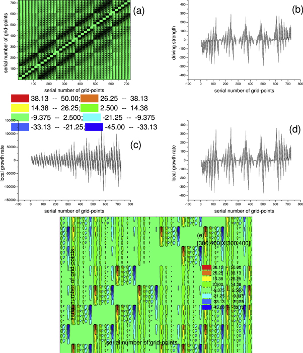
Figure 1. Examples of  Vlasov simulation in Eulerian approach. The profile of dimensionless probability density function
  is represented by its values at discrete points of a grid in the dimensionless
  phase space
  the projection of the grid on the
  plane is a square whose each side contains
  points, and that on the
  plane is a circle
  whose diameter contains
  points, where
  is speed of light in vacuum,
  is the characteristic length proportional to the value of the density
  and
and  represents the maximum of the initial
  -profile
  (a) is for values of these elements of the matrix in equation (2);(b) is for the driving at each grid-point; (c) is for 'local growth rate'
  at each grid-point under strict treatment; (d) is the counterpart of (c) under approximate treatment.(e) is the amplification of the regime around the point
  in (a).
Download figure:
Standard image High-resolution image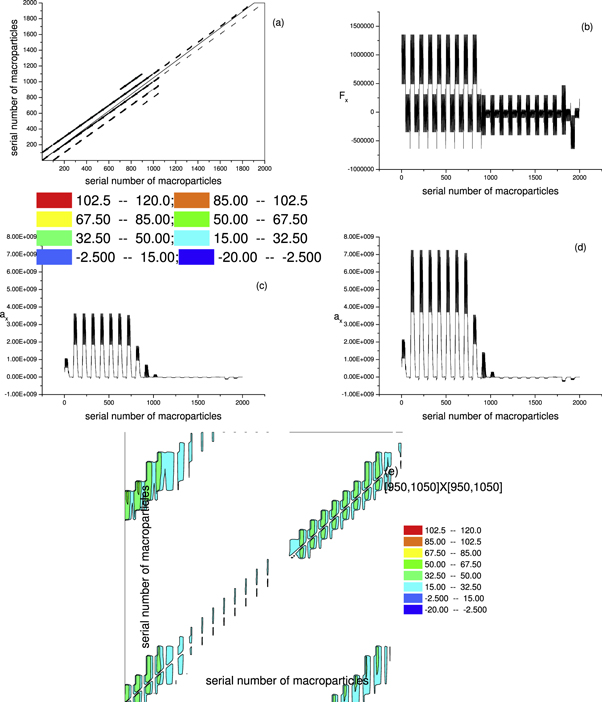
Figure 2. Examples of  PIC simulation. Initially,
  macroparticles are assigned into a
  grid on the
  plane. Self-consistent magnetic field is taken as along
  -direction. (a) is for values of these elements of the matrix in equation (3); (b) is for the driving force on each macroparticle; (c) is for macroparticles' accelerating rate according to strict treatment; (d) is the counterpart of (c) according to approximate treatment. (e) is the amplification of the regime around the point
  in (a).
Download figure:
Standard image High-resolution imageClearly, marked differences exist between results based on different treatments. As shown in figures 1(c), (d), the difference is so large that results in figure 1(c) is higher several orders of magnitude than those in figure 1(d). Moreover, although the curve in figure 1(c) and that in figure 1(d) are in same unit, their shapes are obviously different. Using finer mesh in phase space still faces same problem. Even though results in figures 2(c), (d) are at a same order of magnitude, their relative error is nearly  Figures 1, 2 display examples in
  format. Similar marked differences between results based on different treatments exist universally for EM problem in all formats (from the simplest
  format to
  one) because there is always a high-dimension matrix (due to
  ) no matter which of these formats is studied. For example, a typical
  initial PDF
  where
where  is space-independent, can be represented by a mesh in the
  phase space, and the number of points in this mesh are usually chosen to be up to
  or higher. Because
  implies
  being an asymmetric function of
  and only a space variable
  exists, there are initially a current vortex
  and hence a
  -direction component of
  and a fast growing
  -direction component of
  As previously mentioned, the presence of
  means a high-dimension matrix to be treated when calculating subsequent time evolution of
  According to figures 3(c), (d), strict treatment and approximated one yield obviously different results of the local growth rate. This is similar to what are displayed by figures 1(c),(d). Figure 3(b) displays
  -profile after two time steps
  which exhibits marked space oscillation and hence implies marked density wave.
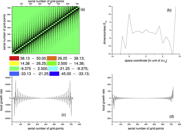
Figure 3. Examples of  Vlasov simulation in Eulerian approach. The profile of dimensionless probability density function
  is represented by its values at discrete points of a grid in the dimensionless
  phase space
  the projection of the grid on the
  axis is a line containing
  points, and that on the
  plane is a circle
  whose diameter contains
  points, where
  is speed of light in vacuum,
  is the characteristic length proportional to the value of the density
  and
and  represents the maximum of the initial
  -profile
  (a) is for values of these matrix elements;(b) is for
  calculated through strict treatment, where
  is in unit of
 and
and  represents the maximum of initial density profile
  (c) is for 'local growth rate'
  at each grid-point under strict treatment; (d) is the counterpart of (c) under approximate treatment.
Download figure:
Standard image High-resolution imageThe root reason for limiting scientific validity of older approximated methods/approaches is to adopt approximation on the coefficient matrix needing diagonalization in discrete expression of the VE, which consists of  -values at
  mesh points of
  phase space:

where  and
and  are steps of the mesh/grid in the phase space, and detailed forms of the function
  and the functional
  can be directly derived from MEs and the functional
  in equations (1), (2). After being aware of this root reason, we diagonalize this coefficient matrix, even though doing so is rather time-consuming, to obtain a set of equations, which are straightforward expressions of
  functions
  in terms of

where detailed forms of the coefficient function  and the functional
  are easily written out but somewhat long for being presented here. Although this straightforward expression is now available, another difficulty still hinders calculating the
  -profile from the
  -profile and the
  -profile (because the time-step
  should ensure
  ) Because the discrete expression is through
  mesh points in
  phase space, the allowed value of
  should be less than the minimum of
  values of
  Usually, a comprehensive discrete expression of a
  -profile should contain those boundary mesh points where
  satisfies. Because not all
  values of
  are
are  once at some boundary mesh points the values of
  are negative, the allowed value of
  will be confined to be
  This difficulty is analogous to the uniform convergence requirement mentioned before.
For the V-M simulation, two difficulties drive us to seek for new ways of describing the evolution of  As shown latter, in a geometric expression of
 expression formulas of
  are converted into those of
  in a same amount. Unlike
  -values mandatory to be
 -value are allowed to be negative. This overcomes the difficulty arising from the requirement that
  should warrant
  being non-negative anywhere.
2.2. Main difficulty in V-M simulation and advantages of combination of different expressions of 

A main difficulty in simulating the V-M system, both in Eulerian approach and Lagrangian one, is to find an efficient expression of  free from being supplemented by unnecessary approximations. In the Eulerian approach, if
  is expressed by a power expansion formula

the VE will act as a recurrence relation/formula defining a set of expansion coefficient functions 
 constructed from this
  -set obviously satisfy the VE. The recurrence relation/formula can lead to a general relation between two expansion coefficient functions with adjacent subindex

which implies  Here,
Here,  and
and  are common expressions of high-order derivatives of
  The convergence condition
 ![${li}{m}_{i\to {\rm{\infty }}}{\rm{| }}\frac{{c}_{i+1}{\left[\upsilon -u\right]}^{i+1}}{{c}_{i}{\left[\upsilon -\vec{u}\right]}^{i}}{\rm{| }}\lt 1,$](https://content.cld.iop.org/journals/2516-1067/4/2/025005/revision2/prexac743eieqn329.gif) whose detailed form is
whose detailed form is  can be warranted if
  can satisfy
  where
where  is speed of light in vacuum. Namely, once
  is convergent with respect to
  it can lead to a set
  warranting the expansion series
  convergent over the region
The power expansion can be converted into another form
where Heviside function is defined as  and
and  and satisfies
  and the coefficient function
  -set can be straightforward transformed from the
  -set.
-set.


where  is from Taylor expansion of
  function. The non-negative-probability requirement demands
  mandatory to be fulfilled [56–58]. Thus, complete microscopic description, which consists of the VE and the non-negative-probability requirement, implies following relation:

where  represents the set of all continuous functions defined over
  -D space
  whose coordinates are
Note that when the operator  acts on
  relevant terms will be in three classes: rising-order terms
  keeping-order terms
  and decreasing-order ones
  Thus, there will be a mono-variable recurrence relation/formula chain

where the functional  represents the recurrence formula reflected by the VE, and expressing
  as
as  is due to the fact that
  can lead to an equation among
  [56–58]

The relation between  and
and  is described as follows: substituting the power series expansion back into Gauss law (where these
  and
and  are space-time inhomogeneous functions and
  is permittivity of free space)

and utilizing  's expression equation (12), we can express
  in terms of
  and hence convert
  into
into  Note that equation (14) is indeed an infinite-order PDE (with respect to
  ) of
) of  and hence often inevitably trigger approximations.
Semi-Lagrangian approaches [43–50, 52–54] face similar difficulty which refers to exact integration of contour of  over
over  -space difficult to be conducted. As a result, even exact functional dependence of
  on
on  can be known from the contour form, it is difficult to obtain exact solution of
  in terms of
The VE reflects global conservation law  and the non-negative-probability requirement
  reflects local positivity-preserving law/requirement [43–50] which is mandatory for applying probability theory to various application issues. Many authors try to take this local positivity-preserving law/requirement into account by adjusting key technical details used in Lagrangian approaches [43–50], such as using more interpolation functions and dividing a time-step into more sub-steps etc Mathematically, these effort choose to update
  in a more complicated manner in which the displacement of a
  -element in
  phase space is a nonlinear function of the time-step
  But these effort also cause computation cost increasing significantly.
Historically, in theoretical plasmas physics, investigations are merely around the VE and hence often drop in a logic contradiction: Starting from the VE, deriving its equivalent equation
  (where
  is the acronym of 'equivalent equation' and the phrase 'equivalent' means no any mathematics approximation being applied and hence can share common solutions with the VE),
 then truncating this equivalent equation to obtain an equation
  (where
  is the acronym of 'truncated equivalent equation' and the phrase 'truncating' means discarding some non-zero terms in the equation and hence cannot share common solutions with the equivalent equation),
 then combining the amputated
  and the VE to obtain solutions of the VE. Obviously, such a procedure is contradict with the fact the a
  cannot share solutions with the equivalent equation
  as well as the VE. Actually, people have been aware of that 'the 'truncation approximation' is a delicate operation, which might lead to a numerical failure of the solution for later times' [20]. Therefore, ignoring the non-negative-probability requirement delays a sound kinetic simulation scheme to be found.
There are different expressions of the PDF  For example, the set
 ![$\{\int {\left[\upsilon -\vec{u}\right]}^{i}f{d}^{3}\upsilon {\rm{;}}i\geqslant 0\},$](https://content.cld.iop.org/journals/2516-1067/4/2/025005/revision2/prexac743eieqn396.gif) where
where  is convenient to reflect the global conservation law, and the set
  is convenient to reflect the local positivity-preserving law/requirement. Compared with sole usage of these expressions, combinative usage of them can avoid unnecessary approximations and is more efficient for establishing a universal and sound scheme of the EM kinetic simulation.
2.3. A compact self-consistent Eulerian expression of

Among different expressions of  choosing the most suitable is important to obtain exact solutions of
  An unsuitable expression will inevitably lead to unnecessary mathematical approximations supplemented. As far as
  is concerned, previously mentioned two Eulerian expressions: mesh expression and power series expressions are far from suitable ones. For example, to make the
  -set certain needs to first make the
  certain from equation (14)), an infinite-order PDE (with respect to
  ) of
) of  and hence often triggers approximations. In contrast, respecting some mathematical features of
  and targeted introducing more suitable Eulerian expression is feasible. For example, because equation (14), or Gauss law, must be respected, the
  -set expression can be further improved into a more suitable expression in which
  is expressed in term of
  itself [59]:

where  is always
  non-negative function
 ![$\left[{H}_{1}+{H}_{0}\right],$](https://content.cld.iop.org/journals/2516-1067/4/2/025005/revision2/prexac743eieqn413.gif) which acts as a conditional probability density function (C-PDF), describes the allocation of particles contained in the
which acts as a conditional probability density function (C-PDF), describes the allocation of particles contained in the  -profile into different values of
  It is straightforward, from the definition formula equation (15), to derive that the non-negative function
 ![$\left[{H}_{1}+{H}_{0}\right]$](https://content.cld.iop.org/journals/2516-1067/4/2/025005/revision2/prexac743eieqn416.gif) satisfies
satisfies ![$\int \left[{H}_{1}+{H}_{0}\right]{d}^{3}\upsilon =1,\int \left[\upsilon -\vec{u}\right]\cdot \left[{H}_{1}+{H}_{0}\right]{d}^{3}\upsilon =0,\left[{H}_{1}+{H}_{0}\right]\left(\vec{u},r,t\right)\equiv 0\equiv \left[{H}_{1}+{H}_{0}\right]\left({\rm{| }}\upsilon {\rm{| }}=c,r,t\right).$](https://content.cld.iop.org/journals/2516-1067/4/2/025005/revision2/prexac743eieqn417.gif) Clearly, such a non-negative function can be constructed from functions in two different classes, one class is denoted as
Clearly, such a non-negative function can be constructed from functions in two different classes, one class is denoted as  and the other
  [56]:
[56]:


and  is
is  while
while  is not. Moreover, it is easy to find, by applying
  -operator and
  -operator on the definition formulas equations (16), (17), that,
  functions:

 and
and  (denoting them as
  ), are alike to
  or satisfy
 ![$\int F{d}^{3}\upsilon =0=\int \left[\upsilon -\vec{u}\right]* F{d}^{3}\upsilon .$](https://content.cld.iop.org/journals/2516-1067/4/2/025005/revision2/prexac743eieqn432.gif) Note that any solution of equation (17) multiplying a
Note that any solution of equation (17) multiplying a  -independent function is still a solution of equation (17), but this important property does not hold for solutions of equation (16).
If an initial profile  can correspond to a
  -set convergent with respect to
  it will yield at least
  initial profiles:


 and
and  Because
 ![$W\left(\vec{u},m\right)\equiv {\int }_{{\rm{| }}\upsilon {{\rm{| }}}^{2}\lt {c}^{2}}{\left[\upsilon -\vec{u}\right]}^{m}{d}^{3}\upsilon $](https://content.cld.iop.org/journals/2516-1067/4/2/025005/revision2/prexac743eieqn443.gif) is a function of
is a function of  and
and 
 is therefore a combination of these functions of
  and
and 

where  and its value equaling to
  implies an equation of combination coefficients
  Likewise,
 ![${\int }_{{\rm{| }}\upsilon {{\rm{| }}}^{2}\lt {c}^{2}}\left[\upsilon -\vec{u}\right]* {H}_{1}{d}^{3}\upsilon =0,$](https://content.cld.iop.org/journals/2516-1067/4/2/025005/revision2/prexac743eieqn452.gif)
 and equation (18) also imply equation of combination coefficients
  If expressing these combination coefficients in terms of power series of
 equations (14), (16) will imply that the
  -profile naturally defines a matrix
  linking the set
  with the set

Now that ![${\sum }_{i\geqslant 2}{\tilde{b}}_{i}\left(\vec{u}\left(r,t=0\right)\right)* {\left[\upsilon -\vec{u}\left(r,t=0\right)\right]}^{i}$](https://content.cld.iop.org/journals/2516-1067/4/2/025005/revision2/prexac743eieqn461.gif) can satisfy equations (14), (16), (17) at
can satisfy equations (14), (16), (17) at  it is easy to prove its counterpart, which is to replace
  with
with  to still satisfy equations (14), (16), (17) at
  We term it as translation operation on the
  -profile and denote it as
  in which
  in
in  is replaced by
  but the matrix linking
  and
and  is as same as that linking
  and
and  Such an operation can be expressed via a formula

and the function  if
if  represents
  (because
  and
and  do not allow
  ), but
  can be not constant-valued if
  represents
  (because
  and
and  allow
allow  ).
).
The matrix linking the  -set and the
  -set reflects geometric/toplogical nature/shape of the
  -profile, and likewise the
  -profile also has a matrix reflecting its geometric/toplogical nature/shape. If this matrix is unchanged during evolution, the related profile is viewed as keeping geometric/toplogical nature/shape. Thus, the phrase 'deformation' refers to this matrix varying with respect to
  and hence the geometric/toplogical nature/shape is not fixed relative to an observer in the
  -frame. Namely, the
  -profile can allow deformation, (relative to an observer in the
  -frame), varying with respect to
2.4. Interpreting the initial-value problem of V-M system in Eulerian-like approach as collective mode in phase space

Because of 
 is therefore not a function positivity-preserving, and hence has zeros, beside
  and
and  in
in  -space. Thus, a typical form of
  or that of functions satisfying equation (17), is

each root  is mono-variable functional of
  and each number
  is repetition index of the root
  (and at least a root satisfies
  ). Such a product
  represents a class of
  -space geometric/toplogic nature/shape. Any
  -independent function multiplying this typical form still satisfies equation (17). From


we can find


and (in similar procedure)


Because of


Equations (24)–(29) will yield


If we use the symbol ' ' to represent the set of functions satisfying equation (17), equations (30), (31) imply that if
  exists, so does
The VE is indeed an expression of the local growth rate ![${\partial }_{t}\left[{H}_{1}+{H}_{0}\right]$](https://content.cld.iop.org/journals/2516-1067/4/2/025005/revision2/prexac743eieqn514.gif) [59]:
[59]:

where the effect of the operator  on a function
  obey following formula [59]


Note that a fraction of the local growth rate

is responsible for  and another fraction

is responsible for the deformation of  relative to an observer in the
  -frame.
Because  must satisfy equation (17), its general form reads
  Substituting this general form into the VE, we have


or

where


and the functional  defined by equation (34) has been contained in
  as well as in
Because of equations (16), (17), (32)–(36), it is easy to find that


, or ![$\hat{{DEGR}}\left[{H}_{1}+{H}_{0}\right]\in \{{H}_{0}\}.$](https://content.cld.iop.org/journals/2516-1067/4/2/025005/revision2/prexac743eieqn525.gif) Therefore, the VE reflects a relation among these members of the set
Therefore, the VE reflects a relation among these members of the set  and has been converted into equation (38), a formal
  st-order ordinary differential equation (ODE) of
  with respect to variable
  Its formal strict solution

reflects a relation between  a member of
  and another member
Asymptotic behavior of  at
at  are
are  and
and  and lead to


which can easily lead to

where  is a constant corresponding to the minimum of all time scales (each represents the time for
 ![$\left[{H}_{1}+{H}_{0}\right]$](https://content.cld.iop.org/journals/2516-1067/4/2/025005/revision2/prexac743eieqn538.gif) at a given coordinate
at a given coordinate  decreasing to

Such a choice of  is for warranting
  non-negative always. Thus, equations (45), (48), (49) reveal that the C-PDF
  corresponds to a time-dependent global oscillation of
  around
  or that of
  around
  Because these fixed points, which correspond to
  exist, the collective mode exhibits as a 'standing-wave' in
  phase space.
Considering the phrase 'Eulerian' is often for describing  by its values at a mesh of the
  phase space, we term above procedure as 'Eulerian-like' because it is based on the description of
  by specified functions defined over the
  phase space. These specified functions reflect geometric/toplogial nature of initial
  -profile. The well-known drawback of the Eulerian approach, i.e., too huge mount of mesh points and corresponding discrete values, is avoided by high-efficiently expressing them through collective mode, represented by the
  -profile, in the
  phase space. Namely, the Eulerian approach is in a one-by-one manner, to update a mesh
  to another mesh
  through a mesh
  Each mesh has its own geometric/tpolgical nature. In contrast, our approach is to utilize respective geometric/topologic nature of three meshes and high-efficiently express the difference
  as a collective mode
  which is determined by
  One-by-one mesh points calculation on individual
  -values is replaced by calculating amplitude of the collective mode. Moreover, compared with various ansatz of
  [40] used in simulating the V-M system,
 ![$f=n* \left[{H}_{1}+{H}_{0}\right]$](https://content.cld.iop.org/journals/2516-1067/4/2/025005/revision2/prexac743eieqn565.gif) is a strict expression. On the other hand, the Lagrangian approach is to express the initial-value problem of the V-M system or the N-M system as those of many initial mono-variable functions (of
is a strict expression. On the other hand, the Lagrangian approach is to express the initial-value problem of the V-M system or the N-M system as those of many initial mono-variable functions (of  ), or Lagrangian particles, identified by different points on a
 -profile. By now, the calculation in the Lagrangian approach is rarely to take into account the geometrical/toplogical nature of this
  initial-values-profile, and to choose a rough treatment in which all initial-value problems of these Lagrangian particles are uniformly/equally treated as having a same time-convergence. This might be an unavoidable difficulty for the Lagrangian approach.
2.5. Example of application of this simulation based on the 5-function expression of

Here, we present some examples of application of this new simulation method. It simulates an electron bunch (e-bunch) travelling within a space inhomogeneous DC-fields configuration. The DC-fields configuration is described as follows:  and
and  if
if  and
and  elsewhere. Namely,
  drops from
  at
at  to
to  at
at  The initial PDF of the e-bunch is
  where
where  and
and  are transverse and longitudinal radius respectively and
  is the global moving velocity (along the
  -direction) of the e-bunch,
  and
and  are initial transverse coordinates of the symmetric axis of the e-bunch relative to the
  -axis. Note that this
  -profile corresponds to initial current profile having a vortex
  As described in last subsection, we can derive, from this initial PDF,
  derivative initial profiles and calculate their evolutions. Some examples are presented in figures 4, 5. Velocity subspace boundary conditions are
 and
and  are finite-valued and
  are always non-negatively-valued. These examples well illustrate that phase space details of the evolving
  -profile can be well reflected by those of the evolving
  -profile.
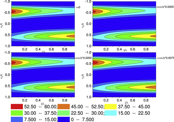
Figure 4. Snapshots of  at
at  where
where  and
and  is the frequency of the oscillation in the off-center density
Download figure:
Standard image High-resolution image
Figure 5. Snapshots of ![$f\left(t,r,{\rm{\upsilon }}\ne u\right)\equiv \left[n-{n}_{0}\right]H$](https://content.cld.iop.org/journals/2516-1067/4/2/025005/revision2/prexac743eieqn603.gif) at
at  where
where  and
and  is the frequency of the oscillation in the off-center density
Download figure:
Standard image High-resolution image2.6. Comparison with others
For comparison with other kinetic simulation schemes, we present, in figure 6, results of applying this method to laser wakefield, a topic attracting many PIC simulations [60, 61]. Electronic density wake of a laser with a triangular-function-type vector potential initial envelope  which is displayed in figure 6(a), has a shape similar to that displayed in figure 1 of [60], For a laser with a Gaussian-function-type initial envelope
  electronic density wake displayed in figure 6(c) has a shape similar to that displayed in figure 19 of [61].

Figure 6. Snapshots of electronic density profile and longitudinal electric field profile of the wakefield of a laser propagating in a plasma layer from left-to-right. (a,b) are at  and for laser initial envelope and plasma parameters in figure 1 of [60]:
  (c,d) are at
  and for initial laser initial envelope and plasma parameters in figure 19 of [61]:
  and same numerical parameters:
  and
and 
Download figure:
Standard image High-resolution image
Because of incomplete information disclosure in these refs, such as missing detailed forms of the interpolation functions used in PIC simulations, it is only possible to make a qualitative comparison. Our results presented in figure 6 also display 'bubble structure' displayed in figure 19 of [61]. But the depth and longitudinal position of density valley differ from those in figure 19 of [61]. For example, in the upper-left panel, the region  is a density valley, it is spaced by a density peak from another density valley at the region
  Likewise, in the down-left panel, a large density valley is at the region
  another small valley is at the region
But in-depth understanding the unavoidable difficulty in particle simulation and seeking for possible solution for it are necessary. A possible solution might arise from a subtle, dual role of an electron. Each electron can be both the source of a scalar potential and that of a vector potential. A notable fact is that scalar potentials from different source electrons will not offset mutually but vector potentials will. This fact implies that the microscopic vector field exerted by an electron can be divided into two parts:  where the subscript 'c' represents 'contributed' (to macroscopic vector field) and 'o' represents 'offset'. For all electrons, there are at least a scalar field and two vector fields defined over the initial phase space
  giving a description on the system. One vector field is from those
  and the other from those
  For example, accelerating rate of each electron
  is a vector, and hence there should be


These unique properties of the  -field can be utilized for solving difficulties mentioned before.
Note that the MEs do not couple with  The uniform convergence requirement forces us to re-consider the role of those RNEs. It is appropriate to view them as a definition of respective
  or all those RNEs yield the expression of an
  -field, which does not couple with the MEs. In other words, the particle simulation can be in a more efficient scheme if noticing the division
  and the fact that the MEs do not couple with
  Ignoring them will make the particle simulation entangled by exactly solving
  from those RNEs. Once the
  field cannot be exactly solved, the whole particle simulation is ruined. Actually, it is unnecessary to bind the particle simulation with this nearly impossible task (because of the uniform convergence requirement). The condition for
  expression formula of
  able to be simultaneously solved, or the fact that those
  (such as

 and
and  ) allow so diverse, even opposite, values of
  lead to an equation of these
  and this equation couples with the MEs to form a natural closure of these
  (because the MEs do not couple with
  ) [56].
3. Summary
Two difficulties previously mentioned limit the validity and efficiency of the EM kinetic simulation in both Eulerian approach and Lagrangian one. This forces us to try more efficient methods on kinetic theory. Starting from a compact expression of  and utilizing geometrical/toplogical nature of initial conditions and conservation laws behind the V-M system, we can take a more efficient form of the initial-value problem of the V-M system. Difference among these
  in the EM kinetic simulation in both Eulerian approach and Lagrangian one are contained in the geometrical/toplogical nature of the
  -profile and are taken into account. The initial-value problem of V-M system is therefore condensed into that of the magnitude of the
  -profile. In short, this new method enables us to consistently treat these
  while treating them through the EM kinetic simulation in both Eulerian approach and Lagrangian one is always perplexed by two difficulties.
Acknowledgments
This work is supported by NSFC.Grant.No.12074398.
Data availability statement
All data that support the findings of this study are included within the article (and any supplementary files).