


Abstract
This study attempts to infer the linkage of sea surface height anomaly (SSHA), surface wind stress and sea surface temperature with the falling ice (snow) radiative effects (FIREs) over the tropical and subtropical Pacific Ocean using CESM1-CAM5 sensitivity experiments with FIREs-off (NOS) and on (SON) under CMIP5 historical run. The obs4MIPs monthly SSH data based upon satellite measurements are used as a reference. The seasonal and annual mean spatial patterns of SSHA difference between NOS and SON are tightly linked to those of SST and TAU over the study domain, in particular, over the south Pacific. Compared with NOS, SON simulates improved seasonal and annual mean SSHA associated with improved sea surface temperature (SST), surface wind stress (TAU) over the trade-wind areas. In SON, the simulated mean absolute bias of SSHA over the study domain is reduced (up to 30%) against NOS relative to observations. The SSHA biases are then compared with CMIP5 models. Despite the biases of SST and SSHA over the south and north flanks of the equator in SON, the seasonal variations of improved SSHA are closely related to those of TAU and SST resulting from the FIREs; that is, higher SSHA is associated with weaker TAU and warmer SST changes and vice versa. The CMIP5 ensemble mean absolute biases of SSHA show similarities to NOS mainly over the south Pacific.
Export citation and abstract BibTeX RIS

Original content from this work may be used under the terms of the Creative Commons Attribution 4.0 licence. Any further distribution of this work must maintain attribution to the author(s) and the title of the work, journal citation and DOI.
1. Introduction
Sea surface height (SSH) is an important climate indicator and has been rising for decades in response to a warming climate, and that rise appears to be accelerating (Church and White 2011, Church et al 2013). Variations of SSH reveal the ocean heat content with warm water being less dense than cold water, so higher SSH areas tend to be warmer than lower SSH areas, affecting the sea level that influences the coastline human activities (Ezer and Atkinson 2014, Sweet et al 2017) and islandic countries (Domingues et al 2018).
Variations of SSH also play a vital role in the climate system by affecting the fluctuations of thermocline depth and ocean currents and affecting model simulations of climate variability, such as El Niño–Southern Oscillation (ENSO) (Rebert et al 1985, Wyrtki 1985, Milne et al 2009) and Interdecadal Pacific Oscillation (IPO) (Ham and Kug 2015, Lyu et al 2016). Li et al (2022) found that the preceding thermocline anomalies (sea surface height anomalies) in the western (eastern) tropical Pacific have a positive (negative) contribution to the discharge phase of ENSO mainly due to the asymmetric wind stress anomalies associated with El Niño and La Niña. Upwelling or downwelling is linked with lower or higher SSH in conjunction with local atmospheric forcings and ocean currents (Liu and Weisberg 2007, Umaroh et al 2017). Spatial distributions of SSH, surface wind stress (TAU) and sea surface temperature (SST) are closely related, especially in the Tropics, according to observational studies (Zhang et al 1997, Casey and Adamec 2002). The prevailing trade winds force the near-surface ocean water westward and further accumulate over the western Pacific warm pool region with higher SSH, accompanied by lower SSH over eastern Pacific Ocean. The changes in SSH that are controlled by the changes in the prevailing trade winds, in turn, lead to the changes in SST (Casey and Adamec 2002, Flato et al 2013, Yang et al 2022).
The reliability of future projections of SSH depends on the fidelity of general circulation models (GCMs) in simulating a realistic present-day SSH mean state. Moreover, model's reproducibility of realistic SSH would further improve simulations of projected climate variability. However, most GCMs exhibited considerable differences in their simulations of present-day SSH mean states (Flato et al 2013). For example, Landerer et al (2014) demonstrated that Coupled Model Intercomparison Project phase 5 (CMIP5) models (Taylor et al 2012) simulated non-trivial SSH anomaly (SSHA) bias against the observation over the tropical region. They found that the SSHA biases were generally associated with the TAU biases. On the other hand, it is reported that the changes in SSH are highly related to the changes in SST under greenhouse warming projections (Dhage and Widlansky 2022).
Because both SSHs and SSTs are affected by modeled surface wind stress (TAU), it is important to know the impact of missing physical processes in the atmosphere on the modeled TAU. Li et al (2014, 2015) found that most CMIP5 GCMs do not consider the falling ice (snow) radiative effects (FIREs), producing too weak TAU and too warm SST over subtropical and tropical oceans (Li et al 2012, 2013) through a mechanism to be described below. The inclusion of FIREs improves model simulated tropical climate states of radiation fields (see SI, figure S1), TAU and SST in CMIP5 (Li et al 2014, 2015, supplementary information (SI)). Li et al (2015) pointed out that CMIP5 models tend to have too strong convection, producing anomalous low-level outflows (figure S2(b)) over the Intertropical Convergence Zone (ITCZ), South Pacific Convergence Zone (SPCZ), and Maritime Continent (figure S3). This leads to weakening surface wind stress (figure S4), and upper ocean mixing, resulting in warmer SSTs (figure S5) over the trade-wind regions (Li et al 2014, 2016, 2018).
Motivated by the aforementioned studies, this study will attempt to infer the extent to which the response of SSHs to the lack of FIREs is linked to weaker surface winds and warmer SSTs. In other words, what are the impacts on local SSH through the remote influence of changes in surface wind stress and SST that are resulted from the FIREs?To address this question, annual-mean spatial patterns and seasonal cycles of mean bias (MBs) and mean absolute biases (MABs) over the study domain (240 °W–0°, 40 °S–40 °N) and, in particular, the south Pacific trade-wind regions (160 °W–120 °W, 30 °S–0 °S) will be examined to understand the biases of the SSHA and their linkage to TAU and SST differences between NOS and SON using obs4MIP AVISO SSH data as a reference, which are based upon TOPEX/Poseidon, Envisat, Jason-1, and OSTM/Jason-2 altimetry measurements.
The influences of surface wind stress and SST on SSHA through the aforementioned radiation-circulation interactions are more apparent over the Pacific basin than over the Atlantic and Indian basins. Over the Atlantic basin, the SSHA is controlled by the surface radiation budget (Li et al 2018) while over the region between the ITCZ and SPCZ of the Pacific, the radiation-circulation coupling is strong (Li et al 2014). Over the Indian basin, there are complex influences such as the Tibet thermal effects and strong seasonal reversal of wind stress and SST. Therefore, we mainly focus on the tropical Pacific in this study.
This paper is structured as follows: section 2 includes a brief description of the data and methodology and model simulations used. Section 3 illustrates the simulation assessment and shows the influence of FIREs on SSHA performance and their links to SST and TAU changes. Section 4 summarizes and discusses the major findings of this study.
2. Reference data, model output and methodology
2.1. Reference data sources and model output
2.1.1. Sea surface height
The obs4MIP SSH monthly dataset is used as a reference, provided by NASA-JPL's Archiving, Validation and Interpretation of Satellite Oceanographic (AVISO) project from TOPEX/Poseidon (AVISO 2011), Envisat, Jason-1, and OSTM/Jason-2 altimetry measurements. This dataset contains absolute dynamic topography (similar to sea level but with respect to the geoid) binned and averaged monthly for the period of 1993–2010. The spatial resolution is 1° × 1° on latitude–longitude grids (https://esgf-node.llnl.gov/search/obs4mips/). Shown in figures S6(a)–(e) are the seasonal and annual mean AVISO SSH distributions over time period from 1993 through 2010.
2.1.2. Sea surface temperature
The monthly sea surface temperature (SST) reference data are obtained from the Extended Reconstructed Sea Surface Temperature (ERSST) dataset (data source: https://www1.ncdc.noaa.gov/pub/data/cmb/ersst/v5/). ERSSTv5 is derived from the International Comprehensive Ocean–Atmosphere Data set release 3.0 SST on a 2° × 2° grid with spatial completeness enhanced using statistical methods (Huang et al 2017, 2018a, 2018b).
2.1.3. Surface wind stress
The surface wind stress (TAU) reference dataset is the Scatterometer Climatology of Ocean Winds (SCOW) based on QuikSCAT measurement (Risien and Chelton 2008). Even though the data period from September 1999 to October 2009 is much shorter than the CMIP models, Lee et al (2013) illustrated that multidecadal variability is not the main contribution for the model bias. As a result, QuickSCAT on 1° × 1° grids could be viewed as the reliable reference data for evaluating model performance and calculating the potential bias.
2.1.4. CMIP5 model output
As shown in table 1, we use 13 CMIP5 (Taylor et al 2012) model outputs in this study. All models except for CESM1-CAM5 listed in table 1 do not include FIREs. To compare with the observation, we select the same period of 1980–2005 in the historical scenario simulation of CMIP5 in their ensemble members designated as r1i1p1f1.
Table 1. List of CMIP5 models used in this study and the corresponding institutes. Only CESM1-CAM5 includes the falling ice radiative effects.
| Model | Institute |
|---|---|
| CESM1-BGC | National Center for Atmospheric Research, US |
| CESM1-CAM5 | National Center for Atmospheric Research, US |
| CNRM-CM5 | Centre National de Recherches Météorologiques/Centre Européen de Recherche et Formation Avancée en Calcul Scientifique |
| inmcm4 | Institute for Numerical Mathematics |
| IPSL-CM5A-LR | Institute Pierre-Simon Laplace, France |
| IPSL-CM5B-LR | Institute Pierre-Simon Laplace, France |
| MIROC5 | Atmosphere and Ocean Research Institute (The University of Tokyo), National Institute for Environmental Studies, and Japan Agency for Marine-Earth Science and Technology, Japan |
| MIROC-ESM-CHEM | Atmosphere and Ocean Research Institute (The University of Tokyo), National Institute for Environmental Studies, and Japan Agency for Marine-Earth Science and Technology, Japan |
| MIROC-ESM | Atmosphere and Ocean Research Institute (The University of Tokyo), National Institute for Environmental Studies, and Japan Agency for Marine-Earth Science and Technology, Japan |
| MPI-ESM-LR | Max Planck Institute for Meteorology, Germany |
| MPI-ESM-MR | Max Planck Institute for Meteorology, Germany |
| MRI-CGCM3 | Meteorological Research Institute, Japan |
| NorESM1-ME | Norwegian Climate Centre, Norway |
| NorESM1-M | Norwegian Climate Centre, Norway |
2.2. Model and sensitivity experiments
2.2.1. CESM1-CAM5 and sensitivity experiments
The National Center for Atmospheric Research—Department of Energy (NCAR-DOE) CESM1 is a fully coupled climate model for simulating the Earth's climate system (for details see section 2 in Li et al (2015)). The descriptions and performance of the cloud-related physical parameterizations in its atmosphere component, CAM5, can be found in Morrison and Gettelman (2008), Gettelman et al (2010), and Lindvall et al (2013). In this study, numerical experiments were performed with the FIREs turned off (hereafter, NOS) and on (hereafter, SON) with the same configurations as in CESM1-CAM5 that participated in CMIP5. The differences in model fields between NOS and SON are referred to as NOS—SON. Both NOS and SON simulations are set up in the same manner as used in CMIP5 'historical' run from 1850 to 2005, exactly the same model components used in the CESM1 contributing to CMIP5, where the same initial fields from preindustrial and the observed twentieth century greenhouse gas, ozone, aerosol, and solar forcing are used (Taylor et al 2012). The simulation time period used in the analyses presented here is 1980–2005.
2.3. Methodology
Following Landerer et al (2014), global mean SSH is removed both in observations and model outputs. Seasonal and annual mean of SSHA shown in figures S6(a)–6(e) are for AVISO, and figures S6(f)–S6(j) for CESM1 NOS and S6k—S6o for CESM1 SON.
We applied three different methods to show the improvements from NOS to SON compared to observations (OBS). The mean absolute bias (MAB) difference, |NOS  OBS|
OBS|  |SON
|SON  OBS|, can be used to indicate improvement from NOS to SON with the positive values. The percentage difference, 100
  (NOS
(NOS  SON)/SON, and the absolute percentage bias, 100
  |NOS
|NOS  OBS|
OBS|  |SON
|SON  OBS|)/|OBS|, are applied to quantify the difference and improvement, respectively.
3. Results
3.1. Seasonal and annual mean spatial patterns
Figures 1(a)–(e) present the seasonal- and annual-mean SSHA differences between NOS and SON (NOS—SON) over the Pacific Ocean. Stippled areas highlight significant differences with t-test at 95% confidence level. The maximum differences are as high as 4 cm. The NOS has lower SSHA in the southwestern Pacific oceans and higher SSHA over the east Pacific trade-wind regions relative to SON. While over the north of the equator, the SSHA east-west patterns are reverse with higher SSHAs over the west Pacific and lower SSHAs to the east Pacific. Moreover, the spatial patterns of significant SSHA differences match well with those of the SST differences with 95% confidence level as shown by the green contours. This is consistent with previous studies, which showed that SST is a vital factor influencing the performance of SSHA and there is a strong linkage of SSH with SST (Landerer et al 2014, Dhage and Widlansky 2022).
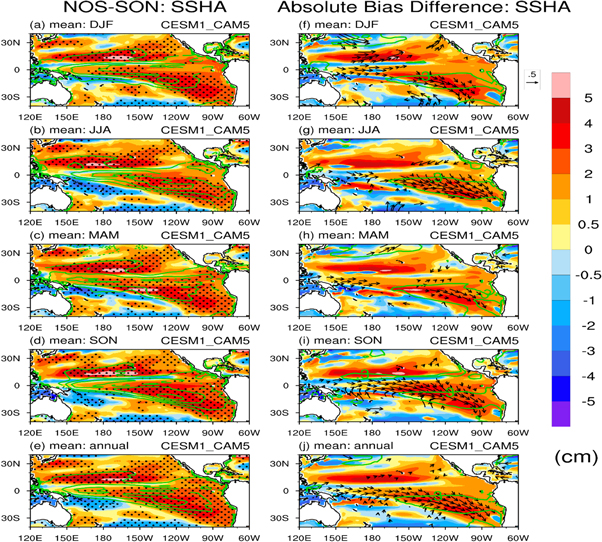
Figure 1. (Left column) Sea surface height anomalies (SSHA: cm) difference between NOS and SON sensitivity experiments using CESM1-CAM5 for (a) DJF, (b) JJA, (c) MAM, (d) SON, and (e) annual mean during the period of 1980–2005. Stippled areas and green lines, respectively, indicate that the SSHA difference and sea surface temperature (SST: K) difference are significant at 95% confidence level. (Right column) Absolute bias difference (|NOS-OBS| minus |SON-OBS|) of SSHA for (f) DJF, (g) JJA, (h) MAM, (i) SON, and (j) annual mean. The green lines represent the absolute bias difference of SST with 0.3 K. The arrow shows the surface wind stress vector (TAU: 50 Nm−2) difference between NOS and SON at 95% significance level.
Download figure:
Standard image High-resolution imageFigures 1(f)–(j) show the mean absolute bias (MAB) differences in SSHA between NOS and SON against observed AVISO SSHA (OBS), i.e., |NOS—OBS|  |SON—OBS|, along with those of SST against ERSST. Note that the positive values of MAB differences in both SSHA and SST represent improvements from NOS to SON. The improved regions in SSHA are found mainly over the south-east and the north-central Pacific off the equator. In particular, the significant differences of surface wind stress vectors with 95% confidence level shown in figures 1(f)–(j) clearly correspond to the significant improvements in SSHA in all seasons and annual mean. Thus, the inclusion of FIREs in CESM1-CAM5 (SON) plays a critical role in reducing the SSHA MABs, which are associated with improved TAU and SST (highlighted with 0.3 K contour) over the same regions. These results are consistent with previous studies regarding the impact of FIREs, i.e., inclusion of FIREs in a GCM improves the TAU and SST over the prevailing trade-wind region and off the coast of the Peru area (Li et al
2020, 2022). We found that without FIREs, the model would have weaker surface wind stress and warmer SST, leading to higher SSHA found in this study, in particular, over the south Pacific Ocean, However, the linkages among SSHA, SST and TAU are not obvious for north-central and south-west Pacific Ocean.
|SON—OBS|, along with those of SST against ERSST. Note that the positive values of MAB differences in both SSHA and SST represent improvements from NOS to SON. The improved regions in SSHA are found mainly over the south-east and the north-central Pacific off the equator. In particular, the significant differences of surface wind stress vectors with 95% confidence level shown in figures 1(f)–(j) clearly correspond to the significant improvements in SSHA in all seasons and annual mean. Thus, the inclusion of FIREs in CESM1-CAM5 (SON) plays a critical role in reducing the SSHA MABs, which are associated with improved TAU and SST (highlighted with 0.3 K contour) over the same regions. These results are consistent with previous studies regarding the impact of FIREs, i.e., inclusion of FIREs in a GCM improves the TAU and SST over the prevailing trade-wind region and off the coast of the Peru area (Li et al
2020, 2022). We found that without FIREs, the model would have weaker surface wind stress and warmer SST, leading to higher SSHA found in this study, in particular, over the south Pacific Ocean, However, the linkages among SSHA, SST and TAU are not obvious for north-central and south-west Pacific Ocean.
To further investigate the linkages between TAU and SSHA, the surface wind stress difference is decomposed into zonal (TAUX) and meridional (TAUY) components shown in figure 2. Both TAUX and TAUY show significant differences with 95% confidence level between NOS and SON for all seasons over the southern hemisphere, especially over the SPCZ, but not over the north flank of the equator. One possible reason is that the surface wind stresses influenced by the more stable anticyclone system persistently over the South Pacific while there are strong seasonal variations of location of midlatitude storms (figures 2(a) and (f)) and small changes in summer (figures 2(b) and (g)) over the north of the equator. On the other hand, in the northern hemisphere winter (DJF), to a lesser extent, MAM and SON, there are significant differences in TAUX and TAUY, which may be influenced by the FIREs (Li et al 2016).

Figure 2. As in figures 1(a)–(e), but for the zonal (a)–(e) surface wind stress (TAUX: 50 N m−2) and the meridional (f)–(j) surface wind stress (TAUY: 50 N m−2).
Download figure:
Standard image High-resolution imageNext, we examine the linkages between SST and SSHA presented in figure S8 of supplementary information. The seasonal-mean SST differences are significant with 95% confidence level between NOS and SON (NOS—SON) shown in figures S8(a)–(f). Improved SSHAs in SON (figures 1(a)–(f)) are collocated over areas with improved SST MABs from NOS to SON except over the north and south flanks of the equator shown in figures S8(g)–(j) for the seasonal mean. That is, the seasonal MAB of SST is reduced from NOS to SON although there exists a remarkable difference between NOS and SON over the north and south flanks of the equator. The SST MABs are reduced significantly (up to 1 K) over the south-east Pacific Ocean, similar to that in figure 7 of Li et al (2015) and figure 8 in Li et al (2020).
To quantify the SSHA differences between the two experiments and the improvement of SSHA, we calculate the percentage difference ((NOS-SON)/SON) and the absolute percentage bias ((|NOS-OBS|-|SON-OBS|)/|OBS|) presented in figure 3. The seasonal and annual differences of SSHA shows at least 5% to 15% between NOS and SON relative to SON with the maximum up to 30% off the coast of America continent such as near the coasts of Peru and California (figures 3(a)–(e)). Similar results can be seen from the absolute percentage biases (figures 3(f)–(j)), indicating improvements from NOS to SON.
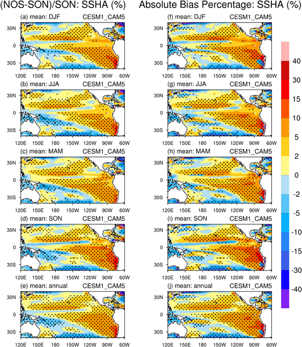
Figure 3. (Left column) The percentage difference ((NOS-SON)/SON) of SSHA between NOS and SON sensitivity experiments using CESM1-CAM5 for (a) DJF, (b) JJA, (c) MAM, (d) SON, and (e) annual mean during the period of 1980–2005. Panels in the right column are similar to those in the left column, but for the absolute bias difference percentage ((|NOS-OBS|-|SON-OBS|)/|OBS|) of SSHA.
Download figure:
Standard image High-resolution image3.2. Seasonal cycle over the South Pacific
Shown in figure 4, we examine the seasonal mean cycles of MBs (4a–4d) and mean absolute bias (|model–observation|) (4e–4 h) of SST, TAU and SSHA for NOS and SON, averaged under four different conditions: (a) southern Pacific Ocean (120 °E–60 °W, 0°–40 °S); (b) regions with positive absolute bias difference (|NOS-OBS|-|SON-OBS|)>0); (c) regions with the wind vector difference being significant at 95% confidence level (area changes with different seasons); and (d) regions with annual wind vector difference being significant at 95% confidence level.
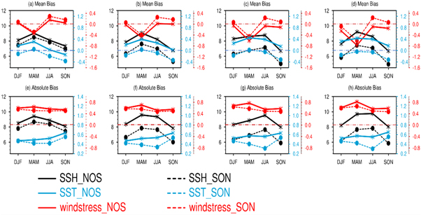
Figure 4. (a)–(d) The mean bias of SSH (black), SST (blue), and wind stress (red) in NOS (solid lines) and SON (dashed lines) experiments averaged over four different selecting areas. (a) averaged over southern Pacific Ocean (120°E–60° W, 0°–40°S). (b) Same as (a) but for the region of positive absolute bias difference (|NOS-OBS|-|SON-OBS|)>0). (c) Same as (a) but for the area that wind vector difference is significant at 95% confidence level (area changes with different seasons). (d) Same as (a) but for the area that annual wind vector difference is significant at 95% confidence level. (e)–(h) Same as (a)–(d) but for absolute bias (|model–observation|).
Download figure:
Standard image High-resolution imageShown in figures 4(a)–(d), in general, the seasonal mean biases of SST, TAU and SSHA in SON are smaller compared to NOS, most importantly, showing similar seasonal variations by increasing SSHA with decreasing TAU and warming SST, and vice versa, under all four averaging conditions. The MABs of SSHA, SST and TAU in NOS and SON averaged over the south Pacific Ocean in four conditions (4e–4h) all indicate improvements in SON against NOS for SSHA, SST and TAU with larger positive MABs in NOS than in SON.
3.3. Annual and seasonal mean spatial patterns of CMIP5 models
Figure 5 shows the percentage differences of SSHA between the ensemble mean of CMIP5 models which do not include FIREs, denoted as CMIP5 against SON. In general, the spatial patterns of SSHA differences between CMIP5 and SON are quite similar to those of NOS and SON with the same order of magnitude compared to NOS versus SON shown in figure 3 except over tropical Pacific, i.e., north and south flanks of the equator. The mean absolute biases of SSHA in SON are smaller than CMIP5 (5–35%) mainly over south of 10 oS, i.e., the South Pacific Ocean, and north of 15 oN, in particular, off the coasts of California and Peru. The performance of SSHA in CMIP5 ensemble over the subtropical Pacific is quite similar to those in NOS and are associated with the biases in CMIP5 SST and TAU shown in Li et al (2015, 2016).
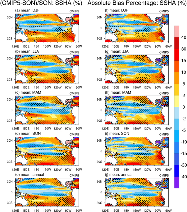
Figure 5. As in figure 3, but for CMIP5 ensemble mean average relative to SON (CMIP5-SON)/SON*100) over 1980–2005.
Download figure:
Standard image High-resolution image3.4. Impact of seasonal footprinting mechanism on SST biases
Additionally, we examine the impact of seasonal footprinting mechanism (Liu et al 2021, Sun et al 2022) on SST biases in the tropics. The warm biases in the tropics can be propagated from the subtropical Pacific according to this mechanism. To isolate the seasonal footprinting mode, we conducted the multi-variate empirical orthogonal function (MEOF) analysis using model simulation output of SST, surface wind stress (TAU), 925hPa winds (u, v) and SSH data from both SON and NOS experiments. Figure 6 shows the spatial distribution of SST anomaly associated with the seasonal footprinting mechanism from SON and NOS experiments, along with their difference (NOS-SON). As shown, the seasonal footprinting mode can be identified from the 2nd mode of MEOF, characterized by a southwestward extension of warm SSTA (in K) from the west coast of subtropical North America. We note that while the variance of seasonal footprinting mode slightly increases from SON (11.8%) to NOS (8.6%), their difference is very modest, with amplitudes of SSTA being around 0.05 to 0.075 ℃, which are much smaller than the absolute biases shown in figures 7(f)–(j). The above result suggests that the biases in the tropics presented in this study should come from the falling ice radiative effect, not the warm biases propagating from the subtropical Pacific.

Figure 6. The spatial distribution of sea surface temperature anomaly (SSTA, in K) associated with the seasonal footprinting mechanism from SON (top-left panel) and NOS (top-right panel) experiments and their difference (NOS-SON, bottom panel).
Download figure:
Standard image High-resolution image
Figure 7. As in figure 1, but for the sea surface temperature (SST: K) for CESM1-CAM5 for NOS and SON.
Download figure:
Standard image High-resolution image
4. Summary and discussion
We investigated the impact of falling ice radiative effect (FIREs) on the sea surface height anomaly (SSHA) over the mid- and tropical Pacific Ocean (120 °E–60 °W, 40 °N–40 °S). We first compared the differences of SSHA, SST and TAU between FIREs-off (NOS) and FIREs-on (SON) sensitivity experiments using CESM1-CAM5 model. It was found that the seasonal and annual mean SSHA differences between NOS and SON (NOS—SON) are tightly linked to those of SST and TAU over the study domain, in particular, over south Pacific oceans. The mean absolute bias of SSHA significantly reduces over the south-eastern and the north-central Pacific Ocean from NOS to SON along with improved performance of SST and TAU. The spatial patterns with significant differences of TAU vectors and SST at 95% confidence level are matched remarkably well with those of SSHA for all seasonal mean and annual mean. These results suggest a strong spatial pattern links that are consistent with the previous studies regarding the links between SST and TAU (Li et al 2014, 2016). That is, the inclusion of FIREs in CESM1-CAM5 improves the TAU and SST over the prevailing trade-wind region and off the coast of the Peru area. Without FIREs included, the model would have weaker surface wind stress and warmer SST, leading to higher SSHA found in this study, particularly over the south Pacific Ocean, However, the linkages between SSHA, SST and TAU are not strong over the north-central flank of the equator, possibly caused by non-trivial biases of SST and TAU both in NOS and SON. We did not find any improvement in SON compared to NOS over the north and south flanks of the equator.
The SSHA MABs in most of the regions show significant improvements with MABs being reduced up to 30% from NOS to SON, particularly over south Pacific and near the coast of Peru area. This result implies that the performance of El Nino-South Oscillation (ENSO) simulation may also be improved in SON compared to NOS since the recharge-discharge mechanism is influenced by the SSHA changes as pointed out by Li et al (2022). In fact, Li et al (2018) found that the CP-ENSO evolution is improved with improved SST and zonal surface wind stress from NOS to SON.
We further examined the seasonal mean variations of mean biases and mean absolute biases in NOS and SON for SST, TAU and SSHA averaged over the southern Pacific Ocean (120 °E–60 °W, 0°–40 °S) under four conditions. We found that both NOS and SON seasonal mean variations of mean bias are the same in NOS and SON with higher/lower SSHA, weaker/stronger TAU and warmer/colder SST. The mean seasonal biases and mean absolute bias of SSHA, SST and TAU are smaller in SON than in NOS, all indicating improvements in SON relative to NOS.
Since there is only one CMIP5 GCM, CESM1-CAM5, that has the FIREs, we used ensemble model mean from those models without FIREs (referred as CMIP5) and compared it to SON. In general, the spatial patterns of SSHA differences between CMIP5 and SON are quite similar with the same magnitude of differences compared to those in NOS—SON except over ITCZ and SPCZ regions. That is, the seasonal and annual mean biases and mean absolute biases of SSHA in CMIP5 are larger (5–30%) than in SON, mainly over subtropics and mid-latitudes south of 10 oS Pacific Ocean and north of 15 oN Pacific oceans. We also found that SSHA shows significant improvement up to 30% in SON against NOS and CMIP5-NOS over the south-east V-shaped regions between ITCZ and SPCZ. It is also worth noting that the most significant impacts of SSHA, SST and TAU variations are located in the V-shaped region as mentioned in Li et al (2014), which highlights the major influenced area of FIREs.
We conclude that in a fully coupled GCM, ignoring the FIREs, the model produces too weak prevailing trade winds and TAU with too warm SST, resulting in anomalously higher SSHA in the CESM1-CAM5 NOS and CMIP5 ensemble mean. It is evident that in SON, the seasonal- and annual-mean spatial patterns and seasonal cycles of MBs and MABs of SSHA, TAU and SST are improved drastically compared to NOS and CMIP5. The present study only examined results from the CMIP5 models. The performance of SSHA in CMIP6 models will be examined in a future study.
We acknowledge that the improved SSHA in SON cannot be solely contributed by the inclusion of FIREs, but may also be contributed by other factors such as ocean circulation, gravitation, and other improved physical processes. For example, the well-known Ekman transport, a component of wind-driven ocean current, is highly related to sea surface height pattern. To elaborate, the dragged upper ocean water would be influenced by the Coriolis effect and move to its right (left) hand side over northern (southern) hemisphere. Once cyclonic (anticyclonic) wind forms near ocean surface, the water tends to be pushed out (into) circulation center and further triggers the upwelling (downwelling). Similarly, Ekman suction and pumping also play vital roles in adjusting ocean circulation and sea surface height over prevailing trade wind area (Talley et al 2011). As a result, the variation of sea surface height is associated with surface wind stress and its Ekman transport, which is beyond the scope of this study.
Acknowledgments
The contribution by JLL to this study was carried out at the Jet Propulsion Laboratory, California Institute of Technology, under a contract with the National Aeronautics and Space Administration (80NM0018D0004) and primary supported by NASA obs4MIPs program, partially supported by NASA Making Earth System Data Records for Use in Research Environments (MEaSUREs), and the NASA Modeling, Analysis and Prediction (MAP), and NASA CloudSat programs. We thank Mr Min-Hua Shen of National Central University, Taiwan for obtaining the seasonal footprinting mode by using the multi-variate empirical orthogonal function (MEOF) analysis.
Data availability statement
No new data were created or analysed in this study.
Supplementary data (1.1 MB DOCX)