

Abstract
Purpose. Soil respiration measurement is an important component of the global carbon cycle assessment. To effectively validate the measurement performance of the monitoring instruments and provide accurate carbon flux data, a new flux-monitoring gas-chamber calibration system was investigated. Method. In an environmentally controlled laboratory, a concentration calculation calibration system, mass calculation calibration system, and flow calculation calibration system were used to quantify soil CO2 emissions. The measurement performance of the soil-respiration monitoring gas chamber was investigated, and the strengths and weaknesses of each calibration system were examined. Results. The unsteady-state flow chamber and steady-state chamber measurements had fewer errors and provided better results than the unsteady-state nonflow chamber. The measured values of the closed chamber were low, whereas the measured values of the open chamber were occasionally high and low. For calibration systems, the concentration calculation system is easy to operate; however, the reference flux values are unstable, and the mass calculation system allows for different gas transport mechanisms. However, it is complex to operate and it is difficult to control the air pressure in the diffusion chamber. The calibration process of the flow calculation system was stable and easy to operate; however, the experimental time was long, and the CO2 gas consumption was high. However, for the calibration effect, the optimal calibration system was the flow-meter algorithm. Conclusion. This study proposes a better calibration method for the soil CO2 flux gas chamber, which is conducive to improving the measurement accuracy of the instrument, and provides new ideas for the calibration of other environmental gas monitoring instruments.
Export citation and abstract BibTeX RIS

Original content from this work may be used under the terms of the Creative Commons Attribution 4.0 licence. Any further distribution of this work must maintain attribution to the author(s) and the title of the work, journal citation and DOI.
1. Introduction
Soil respiration measurements are essential to study the global carbon cycle. Total carbon storage in soils reaches 1394 PgC (Hu 2016), which is approximately three times the total terrestrial biogenic carbon storage (560 PgC) and twice the total atmospheric carbon (750 PgC) (Rustad et al 2000). The annual global CO2 emission from the soil is estimated to be 98 ± 12 PgC (Sahoo and Mayya 2010), making soil one of the major contributors to atmospheric CO2 (Jenkinson et al 1991, Raich and Potter 1995). This accounts for 60%–90% of the respiration of the entire terrestrial ecosystem, which is significantly higher than the annual CO2 released into the atmosphere owing to fuel combustion (5.2 PgC) (Schlesinger and Andrews 2000, Denman et al 2007, Goffin et al 2015). Specifically if the soil CO2 flux monitoring instrument produces a 10% error, the error value is comparable to the total amount released by fuel combustion. Therefore, a small error in soil respiration measurements will have a significant impact on the predicted results of the CO2 concentration in the environment. This further demonstrates that accurate soil respiration monitoring is an important part of the study of global climate change (Forde et al 2019, Abbasi et al 2021, Sanz-Cobena et al 2021).
Currentlythere are many soil respiration (CO2 flux) monitoring methods, including gas chambers, gas wells, and micrometeorology methods. The gas chamber monitoring method is the most widely used, accounting for more than 95% of studies (Luo et al 2001, Craine and Wedin 2002, Knoepp and Vose 2002, Jacinthe 2015, Poblador et al 2017, Buragiene et al 2019, Zhang et al 2022). Primarily unsteady-state gas chambers and open steady-state gas chamber methods are used. Both methods obtain soil respiration data by calculating the change in CO2 concentration over time within the gas chamber; however, the design of the instrument and the choice of calculation model can be flawed in the monitoring process.
Firstly, as the CO2 concentration in the air space of the chamber increases, the concentration gradient of CO2 of the soil surface is reduced thereby inhibiting soil respiration. Choosing a simple linear model as a calculation method would produce significant errors (Gao and Yates 1998, Sahoo and Mayya 2010). Secondly, if the design used to balance the differential pressure between the outside and inside the gas chamber is not reasonable, barometric disturbances or venturi effects can occur during monitoring, resulting in measurement biases that cannot be ignored (Lund et al 1999, Xu et al 2006).Thirdly, whether the gas chamber is designed to allow for accurate flux measurements in a soil environment with gas convection. (Poulsen and Møldrup 2006, Laemmel et al 2019, Levintal et al 2019, Moya et al 2019). Currentlythese issues are not well understood in the design and measurement of gas chambers. Previous comparisons of chambers conducted by other researchers exist in situ, which makes it difficult to eliminate the problem of heterogeneity in instrumental measurements in time or space (Gao and Yates 1998, Lund et al 1999, Xu et al 2006, Midwood and Millard 2011, ). Therefore, absolute calibration systems must be designed for a more accurate and efficient assessment of gas chamber measurements.
Currently, only a few researchers have compared the measured fluxes of monitoring chambers with known fluxes using the gas chamber concentration decay calibration method (Widén and Lindroth 2003, Pumpanen et al 2004). In this study, a more rational and reliable calibration system was designed, and then compared with existing concentration calculation systems for experiments. The advantages and disadvantages of the systems were analysed to improve the accuracy of the flux-monitoring chamber calibration experiment, and reduce the error in the actual measurement of the monitoring gas chamber.
2. Materials and methods
2.1. Calibration device design
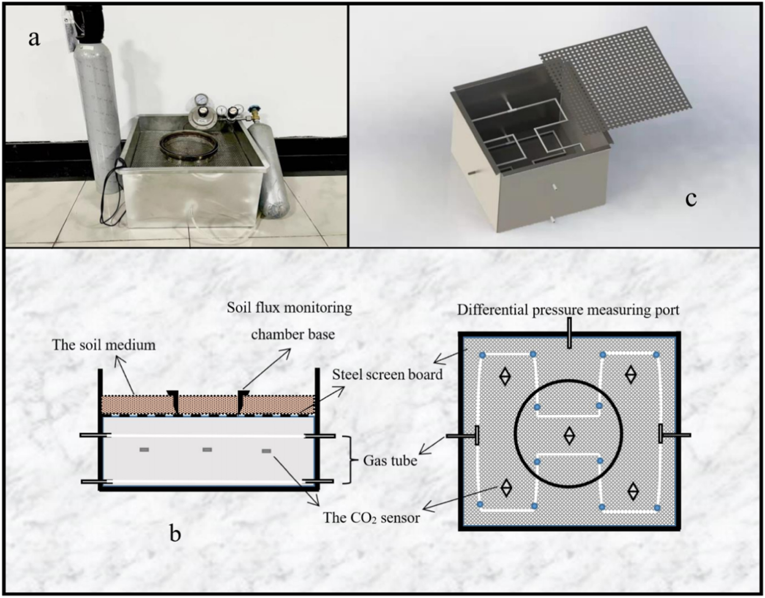
The soil respiration monitoring chamber calibration device consisted of a stainless-steel gas chamber (length 500 mm, width 500 mm, height 300 mm) (figure 1) with CO2, a chamber of 200 mm from the bottom up, and five ventilation tubes of 8 mm diameter and 80 mm length around the chamber. Two of these ventilation tubes were located on opposite sides of the bottom edge of the diffusion chamber at a height of 10 mm, with the inner end connected to a perforated air tube (figure 1(b)). The other three were installed at a height of 170 mm in the diffusion gas chamber, two of which were oriented in the same direction as the bottom ventilation tube, with the inner end connected to a perforated air tube (with the small hole facing down), and the same layout as the small tube at 10 mm. The outer end was connected to the corresponding experimental equipment according to different flux calculation methods. The outer end of the remaining vent pipe was connected to the high-pressure end (H) of the HCS3051 differential pressure sensor (Qingdao Huacheng Measurement and Control Equipment Co., Ltd., China, accuracy ±0.075%), and the low-pressure end (L) of the sensor was connected to a reference system with stable air pressure, which was used to monitor the differential pressure inside and outside the diffusion chamber. A CO2 concentration sensor (model DCO2-TFW1, Beijing Dihui Technology Co., Ltd., China, accuracy ±3% of reading) was installed in the diffusion chamber at a height of 100 mm to monitor CO2 concentration changes in the diffusion chamber (figure 1(b)). Above the diffusion gas chamber was the detection component of the soil flux monitoring chamber. The four corners of the calibration device at a height of 200 mm were pressed with small brackets for placing the steel yarn plate that was not easily deformed. After laying the steel yarn board, a sterilised inactive soil medium was evenly laid on the board at a height of approximately 50 mm, and the monitor base was inserted into the soil beforehand. In this study, experiments were conducted using dry clay soils with the following physical soil parameters: total porosity φ = 0.48, air permeability κ = 10−11 m2, and Hazen effective particle size coefficient (Cu<1.6).
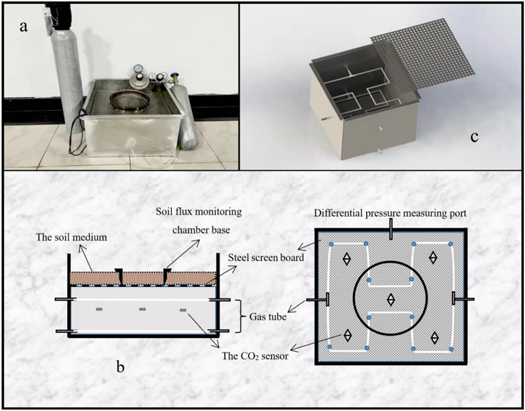
Figure 1. Diagram of the device used to calibrate the soil flux monitoring gas chamber. The schematic diagram of the device (a) shows the main view of the device on the left and top view on the right, where the white lines represent the vent tubes and the small blue dots represent the small vent holes; (b) shows the physical view of the calibration device.
Download figure:
Standard image High-resolution image2.2. Calibration methods
Experiments were conducted between October 2021 and January 2022. To ensure the accuracy of the results, we chose to complete the control experiments in a room with no wind and sufficient space at a room temperature of approximately 15 °C. This study was conducted using gas with a similar CO2 concentration in the soil surface layer (CO2 gas concentration of 4000 μmol.mol−1), and the soil respiration monitor calibration experiment was completed by controlling different aeration conditions. All sensors used in the calibration device were calibrated before each experiment.
2.2.1. Mass calculation method
The experiment started by connecting four ventilation tubes at 10 and 170 mm from the diffusion gas chamber to the CO2 gas bottle with hoses. Subsequently, CO2 from the cylinder was introduced into the diffusion chamber, and the appropriate gas flow rate was adjusted using a controlled gas valve, to present a different concentration range of CO2 in the diffusion chamber for each experiment. Simultaneously, a differential pressure sensor recorded the differential pressure indications between the diffusion chamber and the outside, enabling different soil gas transport mechanisms. The cylinder ventilation strength is divided into three classes: low, medium, and high, which correspond to pressure differences within the diffusion chamber of 0–0.15, 0.2–0.4, and 0.4–0.6 Pa. At this moment, the three classes can be considered as pure diffusive gas transport without gas convection in the soil, gas transport with weak convection, and strong convective gas transport. After waiting for smooth ventilation, the CO2 cylinder was placed on a high-precision electronic scale, model GB10002 (SHINKO ELECTRIC CO., Ltd., Japan, accuracy ±0.01 g), to record the mass of the gas mixture discharged from the cylinder under different ventilation conditions. Specific operation: after the electronic scale reading was stable, the current total mass of the CO2 gas cylinder was recorded every five minutes, and the mass of CO2 gas emitted from the cylinder per unit time was calculated. Simultaneously, the five CO2 concentration sensors in the diffusion chamber were recording the gas concentration in real-time at a sampling frequency of 1s until the gas in the diffusion chamber reached a steady state. The steady-state mark is a change of less than 1% in the indication of the five concentration sensors over a period of 20 min. Here, the amount of CO2 emitted from the diffusion chamber can be calculated according to the law of conservation of the component mass, that is, the amount of gas entering the diffusion chamber is equal to the amount of diffused gas. The CO2 flux fm was calculated as follows (see appendix for detailed steps):

where A is the horizontal area of the diffusion chamber (m2), t is the time (s), Ds is the diffusion coefficient of CO2 (m2.s−1), dρCo/dx is the gradient of CO2 concentration (g.m−4), Co is the concentration of the target gas as it exits the system (cm3.m−3), and uo denotes the velocity of the gas as it exits the system (m.s−1). min is the mass of CO2 gas entering the diffusion chamber (g). In this study, to improve the accuracy of the experimental data, the Kalman filtering algorithm was used to optimise the mass values of gas mixture emissions from the cylinder. It is specifically stated here that the gas flux units (μmol.m−2s−1) of the instrument to be tested were used uniformly to facilitate the later evaluation of the monitoring instrument.
2.2.2. Concentration calculation method
The basic idea of this method is that the CO2 concentration changes with time in the diffusion chamber and the actual carbon flux is calculated according to its changing trend. Specific method: using the same basic operation as described in the mass calculation method, except that the mass of gas emitted from the gas cylinder was not recorded. When the gas in the chamber reached a relatively stable state, the CO2 cylinder was closed and the sampling frequency of the gas concentration sensor was maintained. The equation for actual CO2 flux(fc) is as follows:

where Ct is the CO2 concentration inside the diffusion chamber at time t, V is the volume (m3), and A is the area of the horizontal diffusion chamber. To check the validity of the function, the initial total amount of CO2 (VC0) was calculated and compared with the cumulative sum CT of the discrete function fc (Widén and Lindroth 2003) as follows:

where tn indicates the time required for the CO2 concentration in the box to reach the ambient level.
2.2.3. Flow calculation method
A calibration study was conducted on the apparatus shown in figure 1, where the two ventilation tubes at 10 mm were the inlet, and the two ventilation tubes at 170 mm were the outlet. The two external interfaces of the ventilation tubes at 10 mm were connected to one end of a precision gas flow meter (MF4003-02-O6, Nanjing Shunlaida Measurement and Control Equipment Co., Ltd., China, accuracy ±1.5%) using a tee adapter and the other end of the meter was connected to a CO2 cylinder with a controlled flow rate. The two external interfaces of the ventilation tube at 170 mm were connected in the same way to one end of another precision flow meter, which was then connected to the pump. The outlet of the pump was connected to a 500 ml volume collection device. The CO2 sensor mentioned above was built into a gas collection bottle with a sampling frequency of 2 s to record the CO2 concentration flowing out of the diffusion gas chamber in real time. The other end of the gas collection device was connected to a wash bottle filled with water outside the laboratory to prevent large amounts of CO2 gas from being vented directly into the laboratory and affecting the results.
After the installation of the equipment, the diffusion chamber was ventilated by controlling the gas valve of the CO2 cylinder and adjusting the gas flow rate, while recording the change in the pressure difference between the inside and outside of the diffusion chamber. If the indication was positive, it indicated that the pressure inside the chamber was greater than the external environment. Thereafter, turn on the pump, and according to the inlet flowmeter and differential pressure sensor readings slowly adjust the pumping flow. Finally, the inlet and outlet of the two flowmeter readings are equally adjusted; differential pressure sensor readings did not significantly present differential pressure fluctuations. After adjusting the device, we waited for the CO2 concentration in the diffusion chamber to stabilise, and the flux value was measured and verified at a steady state. The CO2 flux(fv ) is calculated as follows:

where Q is the flow rate of the gas in and out of the diffusion chamber (m3.s−1) because the flow rate in and out can be controlled consistently during the experiment; Cin and Cout denote the CO2 concentration in and out of the diffusion chamber, respectively; A is the horizontal area of the diffusion chamber.
2.3. Tested chambers
2.3.1. Closed chambers
Closed-gas chamber monitoring methods (Knoepp and Vose 2002, Luo and Zhou 2006) can be further divided into non-steady nonflow (NSNF) chambers and non-steady flow (NSF) chambers (Livingston et al 2006). In the experiment, a 300 mm diameter, 150 mm high cylindrical closed (NSNF) chamber was used for the NSNF measurement method. The sensor parameters used were the same as those of the above diffusion chamber. After the gas in the diffusion chamber reached a steady state, the closed gas NSNF chamber was measured 5–7 times at different periods, each lasting 5 min. The carbon flux calculation was also conducted by considering the phase with the greatest rate of increase in gas concentration with time at intervals of half a minute to one minute, and the relevant expressions are similar to equation (2). The measurement data of the NSF chamber were measured using a Li-8100 (Li-Cor Bioscience company in Lincoln, Nebraska). After the gas in the diffusion chamber was stable, five–seven data points were measured and collected three times.
2.3.2. Open chambers
Currently, there are two main types of open chambers (also known as steady-state chambers), and their basic ideas are similar. Both ensure that the monitoring room is close to the external environmental conditions. The principle is designed according to the convection–diffusion equation, that is, when the gas in the system reaches a steady state, the transient term of concentration change with time is zero, and the flux calculation equation is obtained. The difference is that one of them applies a certain gas flow rate to the open gas chamber, which is calculated according to the difference between the CO2 concentration at the inlet and outlet of the gas chamber [flux = (outlet CO2 concentration-inlet CO2 concentration) × flow rate]. Second, after the gas chamber reaches stability, without adding the gas flow rate, the advection-dispersion equation (ADE) has only the diffusion term, that is, div(Ds grad(CCO2)) = 0. The flux value can be obtained by integrating both sides of the equation. Some scholars have added the correction of the environmental pressure disturbance to this flux value for real-time monitoring (Schery et al 1984, Tan et al 2015). This experiment was studied using the first method of flux calculation for open air chambers.
2.4. Data analysis
To show whether the measured fluxes of the monitoring instruments were significantly different from the actual fluxes from the calibration system, the root mean square error (RMSE) and relative error of the measured values of the monitoring instruments were employed to assess their measurement accuracy. The calibration system was judged in terms of the time spent on calibration, complexity of operation, CO2 gas consumption, stability of the flux reference value, and type of gas where the chamber tested the stability of the flux reference value was quantified by the coefficient of variation value. The RMSE and coefficient of variation (C.V) were calculated as follows:


where n is the number of air chamber monitors, Mi is the air chamber monitoring flux value, Ri is the system flux value, σ is the standard deviation of the system reference flux, and μ is the mean system reference flux.
3. Results
3.1. Mass calculation method
3.1.1. Actual flux related data
The mass of the gas mixture discharged from the cylinder was calculated by recording the total weight of the cylinder every five minutes when the gas in the diffusion chamber was in a steady state on an electronic scale. According to the data in table 1 and figure 2, under three different ventilation levels (low, medium, and high), the total mass value of the mixed gas discharged from the gas cylinder in five minutes was relatively stable, and the maximum difference between the measured data under the same ventilation level was at most 0.06 g (6.8% of total mass), and the standard deviation was at most 0.018 g (2%). To further improve the accuracy of the measurement data and eliminate the deviation resulting from external environmental interference, the Kalman optimisation algorithm was used to optimise the emission value of the mixed gas in the gas cylinders under different ventilation intensities. The results are shown in figure 2. This indicates that the gas emission value tends to stabilise after several iterations of the algorithm. The final optimisation data can be considered as the actual emission value of the mixed gas in the cylinder, and the results are presented in table 1.
Table 1. Emission gas-related data table in different convection intensities.
| Level of ventilation | Mass of mixed gas emissions (5 min) | CO2 flux (μmol m−2s−1) | ||
|---|---|---|---|---|
| Maximum difference (g) | Standard deviation (g) | Optimal value (g) | ||
| Low | 0.05 | 0.011 | 1.07499792 | 2.04 |
| Medium | 0.03 | 0.010 | 2.21749271 | 4.21 |
| High | 0.06 | 0.018 | 3.28876718 | 6.25 |

Figure 2. Comparison of the measured value and optimised value of emission gas mass every 5 min under different ventilation levels of CO2 cylinder when the gas in diffusion chamber is in steady-state.
Download figure:
Standard image High-resolution imageAfter obtaining the mixed gas emission values corresponding to different ventilation levels, the actual soil CO2 flux was calculated according to equation (1) (table 1). It can be observed that the carbon flux increases with an increase in the convection intensity (or gas cylinder ventilation level). For CO2 gas with an aeration concentration of 4000 ppm, the soil carbon fluxes corresponding to the three convective intensities were 2.04, 4.21, and 6.25 μmol.m−2s−1, respectively.
3.1.2. Flux monitoring chamber calibration data
The data (figure 3) show that the NSF measurements are better than the NSNF measurements, with the flux values measured by the NSF being closer to the reference values, that is, the measurement bias (relative error) is smaller and its measurements are more stable. The measured value of the open chambers (OC) was slightly higher than that of the closed chambers, but smaller than the reference value in the case of gas convection. Figure 4 shows that under the same mixed gas concentration, the measured value deviation of each chamber increases with an increase in the gas convection intensity (the relative measurement error increased by 9%–30%). When there is no convection (i.e. pure gas diffusion), the measurement deviations of the NSF and OC are significantly small, and the relative errors are −8.3% and +2.5%, respectively, which are significantly close to the reference flux value. The measured values of NSF were slightly lower, whereas that of OC was higher.
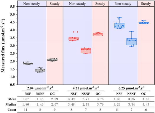
Figure 3. Difference between the measured value and reference flux value of three soil flux monitoring chambers. In systems with reference fluxes of 2.04, 4.21, and 6.25 μmol.m−2.s−1, the measured values of the chambers are counted, results are displayed in the form of a box diagram, and main statistical data are presented in tables.
Download figure:
Standard image High-resolution image
Figure 4. The relative error between a measured value of soil flux monitoring chamber and actual reference flux value. The positive value represents the high measured value and reference value, and the measurement result of the instrument is overestimated; the Negative value indicates that the measured value is lower than the reference value, and the measurement result of the instrument is underestimated.
Download figure:
Standard image High-resolution image3.2. Concentration calculation method
The data in figure 5 show that the overall measurement result of the monitoring chamber calibration experiment using the diffusion chamber concentration calculation method is relatively stable. However, the deviation between the measured value of NSNF and the 1:1 reference line increases with the increasing flux, whereas the measured result of NSF is relatively stable compared with NSNF. In addition, there is no significant deviation with the increase in flux. Compared with the reference flux, there were many low values in the monitoring results of the two closed gas chambers, and the low values measured in the closed nonflow chamber expanded with increasing flux.
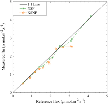
Figure 5. Comparison between the flux measured in the closed non-steady chambers and actual reference flux of the calibration system. There is an overestimation in the measurement results of the instrument, which is higher than line 1:1; Below the 1:1 line, the instrument measurement results are underestimated.
Download figure:
Standard image High-resolution image3.3. Flow calculation method
3.3.1. Actual flux related data
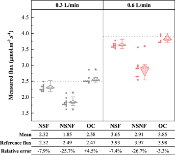
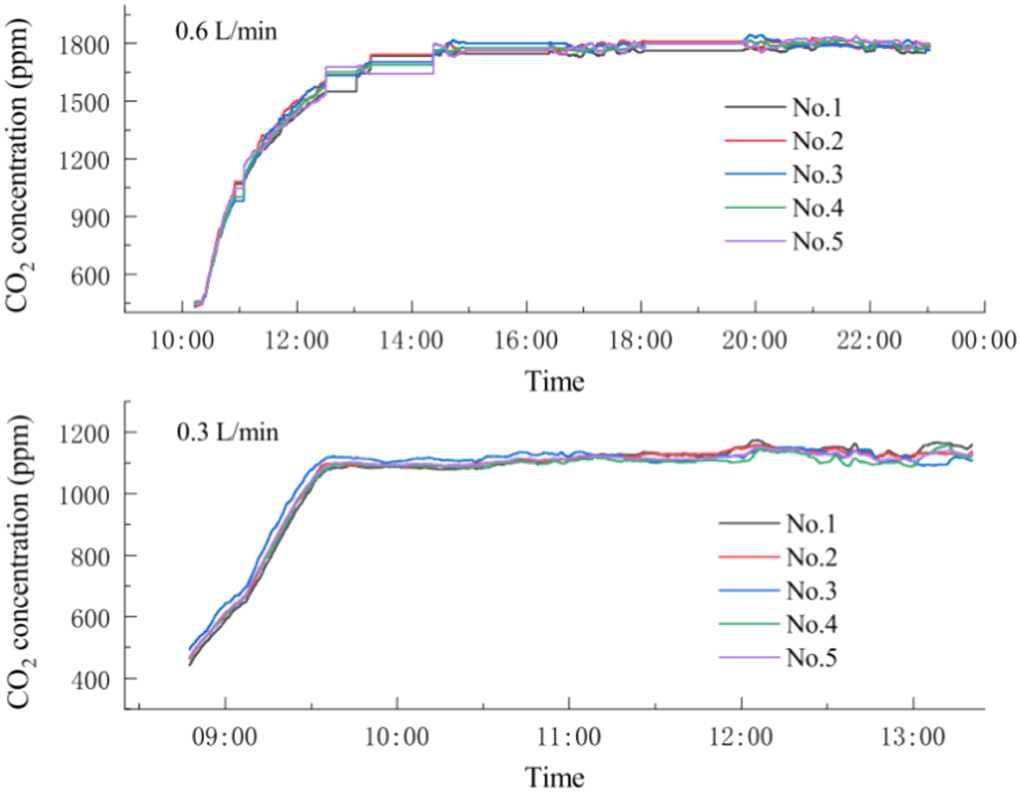
In an environmentally controlled laboratory with a temperature of 15 °C and chamber CO2 concentration of 425 ± 15 ppm, there is no significant gas movement was observed. Furthermore, the experiment used CO2 at a concentration of 4000 ppm as a tracer gas for the calibration study. According to the experimental data in figure 6, when the CO2 in the diffusion chamber was controlled by rates of different gas flow, the steady-state value of the indoor concentration was different. When experiments were conducted at gas flow rates of 0.6 and 0.3 l.min−1, the steady-state values of CO2 concentration in the gas chamber were 1795 and 1168 ppm, respectively. According to equation (4), the actual soil CO2 flux under the two gas flows can be calculated as 2.53 μmol.m−2s−1 (0.3 l.min−1) and 3.94 μmol.m−2s−1 (0.6 l.min−1), respectively.

Figure 6. The function of indoor CO2 concentration with time in the ventilation stage of the diffusion chamber. The curves of five colours represent the data read by the concentration sensors with different numbers, and the stable period of the curve represents that the diffusion chamber is in the steady-state stage.
Download figure:
Standard image High-resolution image3.3.2. Flux monitoring chamber calibration data
To ensure real-time reference flux values, concentration data from various monitoring instruments were selected for calculations during the measurements. It can be observed from the table data in figure 7 that when the gas in the diffusion chamber was in a steady state, its soil gas emissions were relatively stable, and the difference between the CO2 flux before and after was 0.06 μmol.m−2s−1. This value was less than 2% of the average flux value relative to the entire measurement period. According to the data in figure 7, the flux value measured by the NSF (Li-8100) was relatively stable without abnormal values, and the relative error of the measured value was also relatively stable, with a difference between the two errors of 1.3% (the difference in OC between the two measurements reached 7.8%). According to the relative error data in figure 7, the closed-chamber measurements are all less than the reference flux values, and the relative error of the measurement is negative, that is, there is an underestimation of the monitored chamber. The flux values measured in the open gas chamber (OC) were partially greater than the reference flux. When the gas flow rate was 0.3 l.min−1, the average value of the OC measured flux was greater than the reference flux, whereas at a gas flow rate of 0.6 l.min−1, the average flux value appeared to be less than the reference flux, and the measurements were more unstable compared to the NSF. The flux error of the NSNF was the largest, and its flux was less than the reference value, which was significantly underestimated.
Figure 7. Difference between the measured values of three soil flux monitoring chambers and actual reference flux. In Fig, the solid dot represents the measured value of the chamber; the hollow circle represents the average value of the measured results of the chamber; the star represents the measured abnormal value.
Download figure:
Standard image High-resolution image
3.4. Evaluation of gas chamber measurement performance and calibration systems
The data in table 2 show the monitoring performance, that is, the RMSE values of each flux-monitoring instrument in the different calibration systems. The NSF and OC instruments have better monitoring performance compared to the NSNF, with RMSE less than 0.3 and 0.2, respectively, whereas the NSNF monitoring values have a relatively large RMSE. By combining the former relative error data for each air chamber monitoring, it was found that the NSF and NSNF measurements were underestimated, whereas the OC measurements were more diverse (either overestimated or underestimated). In addition, no experiments were conducted on open steady-state gas chambers in the concentration calibration system, as the use of concentration calculations that vary with time is contrary to the principles of OC monitoring.
Table 2. RMSE of carbon flux measurement values from three monitoring instrument.
| Monitoring equipment | Concentration calculation system | Mass calculation system (no convection) | Mass calculation system (convection) | Flow calculation system (0.3 l.min−1) | Flow calculation system (0.6 l.min−1) |
|---|---|---|---|---|---|
| RMSE | RMSE | RMSE | RMSE | RMSE | |
| (NSF) | 0.132 | 0.181 | 0.743 | 0.225 | 0.294 |
| (NSNF) | 0.289 | 0.603 | 1.506 | 0.651 | 1.102 |
| (OC) | — | 0.050 | 0.463 | 0.168 | 0.173 |
The parameter evaluations for each calibration system are listed in table 3. When considering the experiment time, consumables, and operational complexity, the concentration calibration method has an absolute advantage: when considering the stability of the flux reference value of the calibration system and the range of instruments available for calibration, the mass and flow calibration systems are more advantageous, where both have C.V values of 0.01 and 0.008, indicating a relatively stable system and wider range of instruments available for calibration. However, mass calibration systems are limited by the differential pressure between the diffusion chamber and the outside, which makes them relatively limited in the range they can be calibrated to and more complex to operate.
Table 3. Performance evaluation table for each calibration system.
| Calibration methods | Time-consuming | Operation | CO2 consumption a | Stability b | Calibration range | Testable instruments |
|---|---|---|---|---|---|---|
| Mass calculation system | 1–2 h | Complex | Medium (27.3%) | 0.010 | Small | NSF, NSNF, OC |
| Concentration calculation system | < 2 h | Easy | Less (18.2%) | 0.150 | large | NSF, NSNF |
| Flow calculation system | 3–5 h | Easy | Much (54.5%) | 0.008 | large | NSF, NSNF, OC |
a Ratio of the mass of CO2 consumed by each calibration system to total consumption. b Coefficient of variation of the reference fluxes for each system.
4. Discussion
A gas cylinder with a CO2 concentration of 4000 ppm was selected for the calibration experiment because the CO2 gas concentration in the diffusion chamber was more consistent with the CO2 concentration in the actual soil surface, and the carbon flux value was close to the actual soil respiration value. In addition, the gas molecular diffusion mechanism was dominant.
According to the experimental results of the three calibration systems, it can be found that the monitoring effect of NSF (Li-8100) is the most stable. In a pure diffusion environment, the relative error is 7%–9%, which is slightly underestimated. Although the OC monitoring value is closest to the reference value, its actual measurements are subject to overestimation and underestimation, with a wide range of variation and relatively poor stability of the results. The closed NSNF chamber was the worst monitored chamber, with severe underestimation, and its measured values were less stable and prone to anomalous values. For the soil environment affected by gas convection (such as the 'turbulence effect' (Bowling and Massman 2011, Maier et al 2012) or 'barometric pump effect' (Massmann and Farrier 1992, Laemmel et al 2019), each soil flux monitoring instrument will have a certain deviation. In field measurements, the interface wind often causes a certain pressure difference between the soil and surface, which induces gas convection in the soil and enhances the exchange between soil gas and the atmosphere. The result will be a 30%–60% increase in soil gas transport (Laemmel et al 2019). Therefore, gas convection should be considered in the actual measurement, and the monitoring chamber should be improved, or the calculation model should be further corrected for environmental disturbances (Midwood and Millard 2011). Completely open monitoring instruments can be considered to avoid the effects of increased air pressure and concentration build-up in the monitoring chamber on flux measurement data while preventing the phenomenon of enhanced soil gas emissions shielded by a closed gas chamber. When using the closed chamber method to calculate fluxes, a model that is more in line with the actual data can be chosen; it is not limited to linear and exponential models, and multinomial models can also be considered. In the case of unstable measurement environments in the field, it is recommended to conduct multiple monitoring to obtain an average or to perform segmented calculations based on the data to mitigate measurement errors.
For the calibration system, the evaluation and calibration of OC by the concentration calculation method should be further studied because the steady-state monitoring chamber often assumes several hours to reach the steady state, and the monitoring principle of the chamber is contradictory to the calibration method. In addition, owing to the selection of the diffusion chamber concentration attenuation data over time, the proposed combined calculation of flux has a significant impact on the results. The values also changed with different selection times and the reliability of the results was poor. Simultaneously, the soil flux with gas convection cannot be quantified; however, it is convenient for experimental operation and variable control, and the concentration in the diffusion gas chamber can be studied without reaching a steady state. The mass calculation method completes the calibration study of various monitoring gas chambers after the diffusion chamber gas reaches a steady state, and can quantify the soil flux where gas convection exists. However, it was difficult to control the pressure difference inside and outside the diffusion chamber during the experiment. In particular, when studying the pure diffusion soil CO2 emission environment without gas convection, the pressure difference between the diffusion chamber and external environment cannot be eliminated. Meanwhile, the studied flux range is limited, and different CO2 cylinders must be replaced. The concentration in the diffusion chamber was significantly different from that in the field environment. The flow calculation method is based on the law of conservation of the component masses. The difference with the mass calculation method is that this solution allows the valve of the pump to be adjusted to reasonably control the pressure inside the diffusion gas chamber and enables a variety of soil environments to be studied, including both pure diffusion and non-diffusion as well as other complex gas transport situations; however, the Flow calculation method has disadvantages, such as long experimental times and large CO2 gas losses.
5. Conclusion
Flux-monitoring chamber calibration systems are important for environmental gas measurements; thus, it is necessary to ensure that their instrumental measurements are more accurate and reliable. In addition, the calibration system is suitable for CO2 flux monitoring instruments and provides ideas for other gas monitoring or other environmental measurements.
From this experimental study, it can be observed that in a pure diffusion environment, the measurement effects of NSF and OC are better than that of NSNF. The NSF showed a slight underestimation after several experiments, with underestimations of less than 10%, whereas the OC measurements were relatively unstable, with some underestimations and overestimations. However, in soil environments with gas convection, the measurements were all underestimated. For the closed NSNF chamber, the flux measurement error was relatively large and significantly underestimated. Therefore, the monitoring gas chamber should be improved in soil-monitoring environments affected by gas convection, or the calculation model should be modified. In addition, these three calibration methods have advantages and disadvantages for practical operation. If the experimental time and CO2 gas consumption are not considered, then the flow calculation method should be the most appropriate calibration system. The relative concentration calculation method provides a stable calibration effect and comprehensive gas chamber that can be tested. Compared with the mass calculation method, this operation is more convenient, and pressure control in the diffusion chamber is more reasonable.
Acknowledgments
This study was supported by the National Natural Science Foundation of China (grant number: 31971493,31570629). We also thank the editor and anonymous reviewers for their contribution to the peer review of our work.
Data availability statement
The data that support the findings of this study are available upon reasonable request from the authors.
Appendix
According to the law of species mass conservation, the rate of change of the mass of CO2 in the system with respect to time is equal to the sum of the net diffusive flux through the system interface and production rate of the species produced by the chemical reaction. The expression is as follows:

where Cs is the volumetric concentration of CO2(cm3.m−3); ρCs is the mass concentration of CO2 (g.m−3); t is time (s);  is the velocity vector (m.s−1); Ds is the diffusion coefficient of CO2 (m2.s−1); Ss is the mass of CO2 produced per unit volume per unit time in the system. In this study, Ss can be considered as zero and simplified in one dimension for equation (1) as follows:

When the CO2 gas concentration in the control body was in a steady state, the time term in equation (A2) becomes zero. When volume fractionation is applied to both sides of the equation, the equation becomes

where u is the velocity(m.s−1) and ∆V is the value of the control volume. For tiny control bodies, ∆V can be expressed as ∆x·A, where A is the area of the control-volume interface; thus, generating the following equation:

where Ci and Co represent the concentration of the target gas as it enters and leaves the system(cm3.m−3), respectively, and ui and uo represent the velocity of the gas as it enters and leaves the system(m.s−1), respectively. If there is no gas concentration gradient at the inlet, then equation (A4) can be further expressed as:
