

Abstract
One of the main challenges in fMRI processing is filtering the task BOLD signals from the noise. Independent component analysis with automatic removal of motion artifacts (ICA-AROMA) reduces motion artifacts by identifying ICA noise components based on their location at the brain edges and cerebrospinal fluid (CSF), high frequency content and correlation with motion regressors. In anatomical component correction (aCompCor), physiological noise regressors extracted from CSF were regressed out from the fMRI time series. In this study, we compared three methods to combine aCompCor and ICA-AROMA denoising in one denoising step. In the first analysis, we regressed the temporal signals of the ICA components identified as noise by ICA-AROMA together with the noise signals determined by aCompCor from the fMRI signals. For the second and third analyses, the correlation between the temporal signals of the ICA components and the aCompCor noise signals was used as an additional criterion to identify the noise components. In the second analysis, the temporal signals of the ICA components classified as noise were regressed from the fMRI signals. In the third analysis, the noise components were removed. To compare the denoising strategies, we examined the fractional amplitude of low-frequency fluctuations (fALFF) and the overlap between the contrast maps. Our results revealed that including the aCompCor noise signals as regressors in ICA-AROMA resulted in more correctly identified noise components, higher fALFF values, and larger activation maps. Moreover, combining the temporal signals of the noise components identified by ICA-AROMA with the aCompCor signals in a noise regression matrix resulted in deactivations. These results suggest that using the correlation between the ICA component temporal signals and the aCompCor signals as noise identification criteria in ICA-AROMA is the best approach for combining both denoising methods.
Export citation and abstract BibTeX RIS

Original content from this work may be used under the terms of the Creative Commons Attribution 4.0 licence. Any further distribution of this work must maintain attribution to the author(s) and the title of the work, journal citation and DOI.
1. Introduction
The main challenge in processing task-based functional magnetic resonance imaging (fMRI) data is finding the blood oxygen level-dependent (BOLD) signal changes related to the fMRI task out of the noise. In addition to noise coming from the MRI hardware (thermal noise, signal drift, and spikes), fMRI signals contain noise due to motion and physiology (breathing and cardiovascular effects) (Liu 2016 ). The first problem with motion, is that the temporal signal in a voxel originates from a collection of neighboring voxels. This effect was most pronounced at the edges of the brain. Second, spins are excited by successive RF pulses at irregular time intervals due to the movement from one slice to the other. Lastly, motion affects the image susceptibility distortions near the sinuses and ear cavities (Andersson et al 2001). Physiological noise affects the local signal magnetization, T2* relaxation and number of spins due to fluctuations in CBV, CBF, and CMRO2 coming from the cardiac and breathing cycles.
Denoising techniques that correct motion and physiological noise in fMRI can be broadly categorized into three groups: adding noise regressors to the general linear model (GLM), regressing out noise regressors prior to the analysis and using independent component analysis (ICA) (Liu 2016, Parkes et al 2018, Mascali et al 2021).
To determine the motion regressors from the fMRI data, 6 motion regressors (3 rotations and 3 translations) were determined during the realignment step (Siegel et al 2014). Optionally, these motion regressors can be expanded using their temporal derivatives and squared regressors (24 regressors in total). To determine the physiological noise regressors from the fMRI data, anatomical component correction (aCompCor) can be used. aCompCor determines the physiological noise regressors using principal component analysis (PCA) in anatomical areas that are supposed to have no task-related BOLD signals, such as the cerebrospinal fluid (CSF) and white matter (WM) (Behzadi et al 2007). However, increasing evidence suggests that task-related BOLD signals can also be found in WM (Gawryluk et al 2014, Grajauskas et al 2019). aCompCor has been found to provide similar estimations of physiological noise as external recordings (Caballero-Gaudes and Reynolds 2017).
In ICA-based denoising, the fMRI time series are supposed to be a linear combination of independent components, each with its own spatial distribution and temporal signal (McKeown et al 2003). These components can be categorized into task BOLD and noise components. The identification of noise components can be performed manually, which is time consuming and depends on the rater's experience (Griffanti et al 2017), or by using machine learning (ML) (Salimi-Khorshidi et al 2014, Kam et al 2019). A disadvantage of these ML methods is that the machine must be retrained each time the parameters of the fMRI sequence changes (Pruim et al 2015). To avoid this retraining process, Pruim et al (2015) developed ICA-based automatic removal of motion artifacts (ICA-AROMA), in which the noise components are identified based on their high-frequency content (>1 Hz), their correlation with the realignment parameters, and their spatial localization at the brain edges and in the CSF. Noise components can be removed from the fMRI time series, and their temporal signals can be used as noise regressors. Originally, ICA-AROMA was introduced to reduce motion noise.
Because ICA-AROMA is mainly used to reduce motion effects (Parkes et al 2018), it is often combined with aCompCor to reduce the physiological noise. However, because Lindquist et al (2019) showed that performing multiple denoising steps sequentially could result in the reintroduction of noise signals, it is best to combine both denoising strategies into one denoising step. In this study, we compared various strategies to combine ICA-AROMA with aCompCor using fMRI data from a study conducted at our institution (results yet to be published). First, the temporal signals of the components identified as noise by ICA-AROMA and the noise signals determined by aCompCor were combined into one set of noise regressors that were regressed from the fMRI time series. Second, the correlation between the temporal signal of the ICA components and the aCompCor noise regressors was used as an additional argument to identify the noise components in ICA-AROMA. The temporal signals from the components identified as noise by the latter ICA-AROMA were regressed out from the fMRI signals in a second analysis, and these noise components were removed from the fMRI data in a third analysis.
2. Methodology
2.1. Participants
The data for this study was obtained from a fMRI study investigating the effects of transcranial direct current stimulation (tDCS) on episodic future thinking (EFT) (results yet to be published). The included data sets were from 24 females and 6 males (aged 25 ± 3 years) without any neural or psychiatric disorder. All participants were Dutch speaking and right-handed and signed an informed consent form. The current retrospective and the original study were approved by the ethical committee of UZ Brussels.
2.2. MRI protocol
All scans were performed using a GE 3 T MR750W scanner equipped with a 24-channel head coil. For each participant, we selected the T1 BRAVO (TI/TR/TE = 450/8.48/3.23 ms, flip angle = 12°, FOV = 256 × 256 mm2, matrix = 320 × 320, slice thickness = 0.8 mm, 230 slices, NEX = 2), field map (2D gradient echo, TR/TE1/TE2 = 500/4.9/7.4 ms, flip angle = 60°, FOV = 240 × 240 mm2, matrix = 64 × 64, slice thickness/gap = 3.0/0.2 mm, 48 slices, magnitude and phase images), and multi-echo fMRI (ME-fMRI) (gradient echo EPI, TR/TE1/TE2/TE3 = 2000/17/39.2/61.4 ms, flip angle = 70°, FOV = 224 × 224 mm2, matrix = 64 × 64, slice thickness/gap = 3.5/0.0 mm, 48 slices, 210 dynamics) data.
To avoid the effects of the tDCS session on the neural activity, we selected only the data taken prior to the tDCS session. However, since the tDCS session was performed inside the MRI scanner immediately after the selected fMRI scan, all subjects wore MRI-compatible tDCS electrodes (Soteric Medical) attached to the head, with the anode placed at the left dorsolateral prefrontal cortex (DLPFC) and the cathode placed at the right supraorbital. No artifacts were observed in the fMRI images owing to the presence of these electrodes.
2.3. fMRI task
The fMRI task was performed in E-Prime 5 and synchronized with the fMRI scan using a scanner trigger. To allow the scanner to reach steady-state signals, the task started 6 s after the trigger.
During the fMRI scan, the participants performed an EFT task. EFT refers to the ability to imagine events that occur in one's personal future (Schacter et al 2018). EFT is closely related to episodic memory (thinking of one's own past) and uses a neural network comprising the default mode network (DMN): the medial temporal lobe (MTL) including the hippocampus, parahippocampal regions and amygdala, the posterior cingulate cortex (PCC), medial prefrontal cortex (MPFC), and lateral temporal (LTC) and parietal cortex (LPC). Additional EFT activations have been reported in the DLPFC, inferior parietal lobe (IPL), and ventromedial prefrontal cortex (vmPFC).
During the EFT task, a series of 18 common Dutch words was presented on a screen, and the participants had to imagine an associated future event that could happen in their own lives. The participants were instructed that the imagined scenarios must be new, non-repetitive, realistic, limited in time and space and imagined from a first-person perspective (e.g. presented word: car; imagined event: driving to a friend next weekend). Once an event was imagined, the participants had to push a button with their right hand. Each trial lasted 20 s with 4 s rest in between. The presented words were chosen randomly from a list of 72 words per subject.
2.4. Data preprocessing
All fMRI scans were visually checked for artifacts and manually oriented according to the anterior-posterior commissure line with the image origin set in the anterior commissure.
The data were preprocessed using a Nipype pipeline (Gorgolewski et al 2011) based on SPM12 6 and FSL (Smith et al 2004).
The three TE images were combined using a T2*-weighted weighting factor (wi for TEi with i∈[1:3]) (Kundu et al 2017):

with T2* determined by an exponential fit to the TE data from the first dynamic.
Second, the first 3 dynamics were removed as dummy scans. Using the magnitude and phase images from the field map scan, a voxel displacement map (VDM) was created (SPM: FieldMap) and used during the realignment and unwarping step (SPM: Realign & Unwarp) to correct susceptibility distortions (Andersson et al 2003). The SPM ArtRepair tool was used to create movement and frame-wise displacement (FD) plots to determine volume outliers. Based on a visual check of these plots, the data of 2 subjects were discarded from further processing owing to excessive head motion. To avoid adverse effects on the autocorrelation of the time series, no censoring of the volume outliers was performed (Siegel et al 2014, Liu 2016, Parkes et al 2018, Mascali et al 2021). The realigned time series were slice time corrected (SPM Slice Timing) using the slice times found in the json header file.
The T1 anatomical scan was cropped to the brain volume (FSL: robustfov) and the brain was extracted (FSL: BET). White matter (WM), gray matter (GM) and CSF maps were created during the segmentation step (FSL: FAST). The cropped anatomical scan and the tissue maps were coregistrated and resampled to the MNI template (SPM: Coregistration) and the fMRI scan was coregistrated to the resampled anatomical scan. Thereafter, the resampled anatomical scan was normalized (SPM: Normalization) and the normalization parameters were reused to normalize the tissue maps and the fMRI series. Finally, the normalized fMRI data were smoothed using a 6 mm Gaussian filter.
2.5. Denoising
As motion regressors, we used 6 realignment parameters (3 translations and 3 rotations), their temporal derivatives, and squared regressors (24 regressors in total). Given the BOLD signals reported in WM (Gawryluk et al 2014, Grajauskas et al 2019), we used the temporal signals of 5 PCA components determined in the CSF using aCompCor, as physiological noise regressors.
For the ICA-AROMA analyses, the ICA components were determined using FSL Melodic. Using the script 7 of Pruim et al (2015), the noise components were identified as noise based on their location at the brain edges and in the CSF, the amount of high-frequency (> 1 Hz) content, and their correlation with noise regressors. In the first ICA-AROMA (ICA-AROMA-1) analysis only the 24 motion regressors were used as noise regressors. In the second ICA-AROMA analysis (ICA-AROMA-2), the 24 motion and 5 aCompCor signals were used as noise regressors.
As reference from the current practice, in the first analysis the temporal signals of the noise components determined by ICA-AROMA-1 and the five regressors from the aCompCor analysis were regressed out (nilearn: clean_img) from the fMRI signals (ICA-AROMA-1/regression). As alternative strategies, only the temporal signals of the noise components identified by ICA-AROMA-2 were regressed out (nilearn: clean_img) from the fMRI signals (ICA-AROMA-2/regression) in the second analysis and in the last analysis, the ICA components identified as noise were non-aggressively removed (FSL: fsl_regfilt) from the fMRI data (ICA-AROMA-2/removal).
2.6. fMRI processing
The fMRI data were processed using SPM12. For each subject, a design matrix was built based on the EFT trial onsets and durations. The duration of each trial was defined as the time between the onset of the presented word and the button response. In the case of a missing response, the average response time for that participant was used.
The individual activation (positive model fit: EFT > 0) and deactivation (negative model fit: EFT < 0) contrast maps were thresholded using a voxel significance threshold of p(uncorrected)<0.001. A weighted overlap map (WOM) per contrast was created (Seghier and Price 2016) as
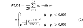
(wi: weighting factor depending on the significance pi of the contrast for subject i (i∈[1:28]))
One-sample t-tests were performed based on the individual contrast maps. To reduce the chance of false positive results, the group statistical maps were thresholded using a voxel significance threshold p(uncorrected)<0.001 combined with a WOM mask (WOM > 10%). This threshold was based on the Monte Carlo simulations of 1000 studies done on 28 subjects using RepSim 8 . Per study, 28 contrast maps were simulated and thresholded at p(uncorrected)<0.001, a WOM was determined and a 1-sample t-test was performed to simulate the group analysis. The resulting statistical map was thresholded at p(uncorrected)<0.001. The Monte Carlo simulations revealed that the chance of having a repeated false result in 3 subjects (∼10% of 28) in combination with a false positive group effect in at least 1 voxel is 0.18. On average, this corresponded to 1 ± 2 voxels per simulation.
2.7. Comparison of the denoising strategies
To compare the fMRI results after applying the various denoising strategies, we calculated the global fMRI signal as the averaged signal over the entire brain. For this global signal we calculated the temporal signal-to-noise ratio (tSNR) and the fractional amplitude of low-frequency fluctuations (fALFF). The fALFF is defined as the power within the BOLD frequency range (0.08–0.1 Hz) over the total frequency power. The tSNR and fALFF values were compared pairwise between the three denoising strategies.
At last the overlap between the resulting group activation and deactivation maps were determined.
3. Results
3.1. Identification of the noise components
The fMRI series were split into 47 ± 18 components by Melodic. ICA-AROMA-1 identified 21 ± 15 components as noise components. ICA-AROMA-2 identified 22 ± 15 components as noise components. In 16 subjects, no differences were found in the classification of the components. In the others, 1 to 6 components were identified as noise by ICA-AROMA-2 but not by ICA-AROMA-1. Visual inspection of these latter components confirmed their classification as noise.
3.2. Pairwise comparison of tSNR and fALFF
As can be seen in table 1, tSNR was significantly higher in ICA-AROMA-1/regression than in ICA-AROMA-2/regression and ICA-AROMA-2/removal. The tSNR in ICA-AROMA-2/regression was significantly higher than in ICA-AROMA-2/removal. The fALFF in ICA-AROMA-2/regression and ICA-AROMA-2/removal was significantly higher than in ICA-AROMA-1/regression.
Table 1. Overview of the results found for the pairwise comparison of tSNR and fALFF between ICA-AROMA-1/regression, ICA-AROMA-2/regressions and ICA-AROMA-2/removal. The reported p-values are Bonferroni corrected and the size of the found effects is given by a Cohen d-score.
| tSNR | fALFF | |||||
|---|---|---|---|---|---|---|
| t | p | d | t | p | d | |
| ICA-AROMA-1/regression - ICA-AROMA-2/regression | 9.26 | <0.001 | 1.75 | −9.25 | 0.001 | 1.75 |
| ICA-AROMA-1/regression - ICA-AROMA-2/removal | 3.78 | 0.009 | 1.76 | −7.70 | <0.001 | 1.45 |
| ICA-AROMA-2/regression - ICA-AROMA-2/removal | 3.78 | 0.009 | 0.71 | −2.13 | 0.52 | 0.40 |
3.3. Overlap between the activation and deactivation maps
In 1528 voxels, a significant activation was found for ICA-AROMA-1/regression, of which 97% overlapped with the activations found in ICA-AROMA-2/regression and 95% overlapped with those of ICA-AROMA-2/removal. 8723 voxels showed a significant activation in ICA-AROMA-2/regression, of which 17% overlapped with the activations found in ICA-AROMA-1/regression and 79% with those found in ICA-AROMA-2/removal. In ICA-AROMA-2/removal, 14890 voxels showed a significant activation, of which 10% overlapped with the activations found in ICA-AROMA-1/regression and 47% with those found in ICA-AROMA-2/regression. ICA-AROMA-1/regression revealed a significant deactivation in 864 voxels, while only in 4 voxels a significant deactivation was found in ICA-AROMA-2/regression and none in ICA-AROMA-2/removal. The 4 voxels of ICA-AROMA-2/regression overlapped with the deactivations of ICA-AROMA-1/regression. None of the deactivations found in ICA-AROMA-1/regression overlapped with the activations found in ICA-AROMA-2/regression or ICA-AROMA-2/removal. The overlap between the activation and deactivations maps is shown in figure 1.

Figure 1. The activation maps found in ICA-AROMA-1/regression (red) and ICA-AROMA-2/regression (blue) (A), ICA-AROMA-1/regression (red) and ICA-AROMA-2/removal (green) (B) and ICA-AROMA-2/removal (green) and ICA-AROMA-2/regression (blue) (C) overlaid on each other to show their mutual overlap. Figure D shows the deactivation map found in ICA-AROMA-1/regression (red). All activation and deactivation maps present the voxels that showed a significant group result at p(uncorrected)<0.001 and WOM > 10%.
Download figure:
Standard image High-resolution image
4. Discussion
In this study, we compared multiple strategies for combining ICA-AROMA and aCompCor denoising in a ME-fMRI experiment. Our results showed that all denoising strategies yielded overlapping activation maps. However, the extent of the found activation differed largely with the smallest activation map found in ICA-AROMA-1/regression and the largest found in ICA-AROMA-2/removal. A possible explanation for the observed difference could be the partial removal of task signals due to noise regression (Fox et al 2009, Murphy et al 2009, Pruim et al 2015, Liu 2016, Mayer et al 2019). This hypothesis was supported by the observed lower fALFF values in ICA-AROMA-1/regression.
Since ICA-AROMA identifies noise components based on their spatial location at the brain edges and in CSF and by their high-frequency content (Pruim et al 2015), ICA-AROMA-1 has already classified most of the physiologic noise components correctly as noise. The fact that in half of the subjects, no additional components were classified as noise by ICA-AROMA-2, supports this hypothesis.
The smaller activation map and the deactivation map found in ICA-AROMA-1 suggest that combining the temporal signals of the noise components identified by ICA-AROMA-1 with the aCompCor noise signals in the noise regression matrix, could have impacted the fMRI results negatively. In contrast, Parkes et al (2018) reported consistent results for ICA-AROMA when various amounts of physiological noise regressors, defined as a global signal or determined with aCompCor, were regressed out in a separate denoising step. Our results suggest that including the aCompCor signals as regressors in the ICA-AROMA step would be a better approach.
Although, including the physiological noise signals from aCompCor as regressors in ICA-AROMA seems to improve the classification of noise and non-noise components, one should keep in mind that ICA often has difficulties in splitting noise and neural activity in separate components (Beall and Lowe 2010, Caballero-Gaudes and Reynolds 2017). As a result, studies (Dipasquale et al 2017, Parkes et al 2018, Mayer et al 2019, Mascali et al 2021) comparing various denoising strategies often found that ICA-AROMA performed moderately compared to the others. The improved classification of the ICA components by including physiologic noise regressors, could be of help when training machine or deep learning based ICA denoising algorithms (Salimi-Khorshidi et al 2014, Kam et al 2018).
In this study, we used a ME-fMRI sequence. Compared with single-echo fMRI (SE-fMRI), ME-fMRI has the added advantage of reducing thermal noise (Dipasquale et al 2017, Kundu et al 2017). Combining ME-fMRI acquisitions with ICA-based denoising (ME-ICA and ME-ICA-AROMA) has been shown to be powerful in reducing motion and physiological noise (Caballero-Gaudes and Reynolds 2017, Kundu et al 2017).
5. Conclusions
In this study, we compared multiple strategies to combine ICA-AROMA and aCompCor denoising. Our results suggest that including the aCompCor noise signals as regressors to identify noise components in ICA-AROMA in combination with the removal of the identified noise components performs best.
Acknowledgments
The ME-fMRI sequence used in this study was provided by GE as a research key.
Data availability statement
The data that support the findings of this study are available upon reasonable request from the authors.
Ethical statement
This study was performed in accordance with the Declaration of Helsinki and was approved by the ethical committee UZ Brussels. All participants signed an informed consent.
Funding sources
This research did not receive any specific grants from funding agencies in the public, commercial, or not-for-profit sectors.
Declarations of interest
None.
Footnotes
- 5
E-Prime: https://pstnet.com/products/e-prime/ (accessed 13 October 2021).
- 6
SPM12: http://www.fil.ion.ucl.ac.uk/spm/ (accessed 13 October 2021).
- 7
ICA-AROMA script: https://github.com/maartenmennes/ICA-AROMA (accessed 13 October 2021).
- 8
RepSim: https://github.com/P-VS/RepSim (accessed 13 October 2021).