


Abstract
The EEG is an important noninvasive brain signal measured from scalp electrodes with the potential for application in the diagnosis of neurological and mental health disorders. In this context analysis of the spectral properties of the EEG are an important aspect of understanding the signal. One characteristic of the signal that has been observed is the presence of intermittent periodicity or regular oscillatory activity under certain conditions. Typically, though not always, this periodicity occurs at ∼10 Hz (called alpha oscillations) and is observed most reliably under eyes closed conditions as a peak in the power spectrum. In the literature the alpha oscillation is generally characterized by the power in the relevant band of the power spectrum. However, since it occurs embedded within a background of nonperiodic activity with a 1/fγ spectral envelope, this approach does not separate the oscillation from the background nonperiodic activity and therefore provides an imprecise view that is largely determined by the spectral decay rather than the embedded periodicity. Here we present an approach to assess periodicity in the EEG signal that is robust to distortions by changes in the 1/f background nonperiodic activity and is particularly suited for detection of small peaks where the band is overwhelmed by the background decay. The method utilizes the second order derivative of the FFT of the signal autocorrelation to define the resulting metric 'Oscillation Energy' (or Eα for alpha oscillations). We demonstrate its performance compared to several variants of traditional power spectrum measures with simulated signals and show its application to example EEG signals. We believe a more precise metric to characterize peaks arising from periodicity like this will enable researchers in the field to develop a clearer understanding of this feature of the signal and its relation to behaviors.
Export citation and abstract BibTeX RIS
1. Introduction
The purpose of this paper is to establish a new metric for detecting and quantifying peaks in the power spectrum in a manner that is separated from the background envelope. Typically this would represent a characterization of peaks arising from periodicity or oscillations, such as the alpha oscillation, that are embedded within the EEG signal, while minimizing the contribution of background nonperiodic activity.
The EEG is a composite of spiking activity, synaptic and glial generated currents, macro field fluctuations, head geometry and volume conduction effects. While there has been obvious periodicity observed in the EEG since its discovery [1], much of the signal is not periodic in nature but rather composed of complex nonperiodic components. Indeed, the underlying local field potentials (LFPs) that represent field activity on the cortical surface, and therefore do not include influence of head geometry or skull conductivity, have been shown in monkeys to be composed of spectrally complex propagating waveforms [2–4]. This phenomenon has also been demonstrated in human ECOG recordings on the cortical surface [5]. Together this suggests that the signal is not simply composed of independent superimposed periodic signals, but rather an envelope of complex waveforms of mixed frequencies with varying phase relationships. On the other hand, there is also evidence of oscillations in neuronal synchronization that are related to the LFP [6], although the relationship between spike firing and LFPs is complex [7, 8]. Altogether the evidence suggests EEG is more likely a composite of complex nonperiodic waveforms along with embedded oscillatory or periodic components rather than simply a superposition of independent periodic components.
1.1. Confounding of oscillations and non-periodic components
Despite the mixing of periodic and nonperiodic components, EEG as a field has come to confound these aspects, referring to broad bands of the aggregate power spectrum or power spectral density (PSD) as oscillations. Such spectral decomposition historically gained popularity in the field of radio transmission and was used in teasing apart periodic components. However, when applied to complex nonperiodic signals like the EEG, interpretation must be more careful.
The convention that has emerged in the EEG field is to divide the power spectrum into broad bands of different frequency ranges and refer to each of these bands as 'waves' or 'oscillations' within that range. This definition has its origins in its early history in the 1930s and 40s when the absence of computers necessitated simplifications based on visually recognizable aspects of the signal [1, 9–11]. The tedium of performing manual computation on a signal obtained on a film or ink writing oscillograph gave rise to photomechanical frequency analyzers (e.g. the Walter and Kaiser analyzers) that produced outputs of particular signal bands directly on the oscillograph [10, 12]. Due to cost and technical constraints these analyzers had to limit to broad band analysis with pre-specified ranges. While the early researchers who built these analyzers warned of its limitations, particularly in application to more complex nonperiodic signals like the EEG [9, 10, 12], it has nonetheless become convention over the subsequent decades leading to use of language with an implicit supposition that the signal entails propagating waves of a particular frequency range where one frequency band is in essence independent of another.
1.2. Structure of the EEG signal
The PSD of the EEG signal is typically a decreasing function with lower power at higher frequencies [13]. This decay in the PSD approximates, but does not strictly conform to, a 1/fγ pattern (example shown in figure 1(A) red). Such 1/f structure implies underlying temporal correlations between the frequencies and reinforces a complex relationship between them [14], although the origin of this structure is still very much a subject of debate [8, 15, 16]. In human EEG the exponent γ that defines the steepness of the 1/f decay in the 2–25 Hz range can have a broad range of values from 0.5 to 2.25 across individuals and conditions [17]. However, under certain circumstances, periodicity or oscillations become evident in the signal. This periodicity, when it emerges and is strong enough, reflects as a peak in the power spectrum of the EEG signal over and above the 1/f-like spectral envelope (for examples see figures 4(D)–(F)). Periodicity is most evident in the signal when visual activity is blocked (eyes closed) and is typically around 10 Hz (within the alpha band, defined as the range from 7 to 15 Hz or 7.5 or 8 to 12 or 13 Hz depending on research group since the band delineation is not always agreed upon) [18–20]. Less frequently, it can arise in other ranges as well or at multiple frequencies as we demonstrate below.
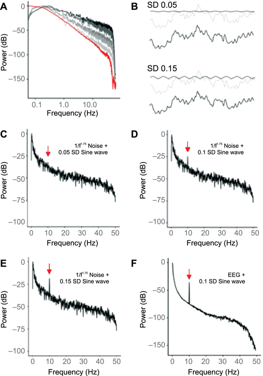
Figure 1. Simulating colored noise with an embedded oscillation. (A) Power Spectrum of colored noise (noise generated with 1/fγ spectrum) with γ ranging from 1 (black) to 2 (grey), as well as the power spectrum an example real EEG trace (red; γ = ∼1.75). Note both axes are shown in log scale. (B) Examples of 10 Hz oscillations (black) with amplitudes of different standard deviations of the noise signal (grey; top 0.05SD, bottom 0.15SD). Signals added together with the oscillation are shown below (black) against the original trace (grey). (C)–(E.) Power spectrum of colored noise signal with γ = 1.75 and added 10 Hz oscillation with amplitude 0.05 SD (C), 0.1 SD (D) and 0.15 SD (E) of the noise signal. (F) Power spectrum of EEG signal (without any detected intrinsic oscillation) with added 10 Hz oscillation with amplitude 0.1 SD of signal.
Download figure:
Standard image High-resolution imageHowever, spectral analysis methods typically used in EEG analysis do not separate such embedded oscillations from the background spectral activity. Researchers interchangeably use the term 'alpha waves' and 'alpha oscillations' to refer to the sum of the PSD across the alpha range of frequencies. This is so regardless of whether there is indeed an evident oscillatory component or not and irrespective of where the peak occurs within this range. However, as we will demonstrate here, the power of the alpha band is largely a reflection of the overall decay of the nonperiodic 1/f spectral envelope than the emergent periodic component. Alpha power as a measure is therefore not particularly sensitive to the oscillatory component and therefore misses important distinguishing information.
Here we define a method that can better isolate the peak or oscillatory component from the overall spectral envelope, defining a new measure which we term the oscillation energy or Eo. Other methods [21] have approached this challenge of estimation of the peak in isolation by subtraction of the background activity using sophisticated curve fitting. Our method represents an alternative approach that is more sensitive to detection and discrimination of small peaks that may be overwhelmed by the background and is relatively insensitive to the shape of the background activity.
2. Description of method
The method described here enables separation of peaks, typically representing embedded oscillations, from a largely non-periodic background envelope of the EEG signal. It is intuitively simple in that it amplifies and separates out the peak in the power spectrum from the background 1/f envelope. The metric obtained is a measure that we have termed oscillation energy (or Eα, when applied to the alpha band) and can be thought of as an indication of both the strength and fidelity of an embedded oscillation above the complex 1/f background activity.
We demonstrate our method first with simulated signals followed by a view of its application to real EEG signals.
2.1. Simulating  noise with embedded oscillations

We demonstrate our method using simulated colored noise with a 1/fγ, structure in the power spectrum (i.e. gaussian distributed noise with a power law spectrum), embedded with a 10 Hz sine wave. We generated this colored noise with γ varying from 1 to 2, which is the typical range for the slope of the PSD between 2 and 24 Hz for resting state EEGs [17]. To do so we used the python library colored noise 1.0.0 (https://pypi.org/project/colorednoise/) that is based on the algorithm defined by Timmer and Koenig [22]. Briefly, this method generates pseudo-random numbers, multiplies these numbers with a curve typical for that decay or γ value and then normalizes them. We then applied a band pass filter to the generated signals between 1 and 50 Hz as is typical in EEG studies, utilizing a total signal length of 3 minutes.
The power spectral density or PSD of these simulated signals is shown in figure 1(A) (grey to black) alongside the PSD of an actual EEG signal (also three minutes in duration, 14 channel recording) that shows no evidence of an oscillation (red). In this case the PSD was computed using the standard Welch method (8 segments with hamming window and 50% overlap). The example EEG signal approximates a decay exponent γ of 1.75. (Note the log scales for both axes in contrast to the semi-log scale in other panels in this figure).
Each of these signals was then added together with a 10 Hz sine wave with a range of amplitudes. Specifically, the amplitude of the sine wave was varied from 0.05 to 0.2 times the standard deviation (SD) of the amplitude distribution of the original signal. Figure 1(B) shows an example of a power noise signal with γ = 1.75 overlaid with the sine wave (above) along with the aggregate signal overlaid on the original signal (below). The two examples shown are for sine waves of amplitude 0.1 (top) and 0.2 (bottom). As can be seen, at these amplitudes, the added oscillatory activity is barely visible to the eye in the aggregate signal. However, it is evident in the PSD as a sharp spike at 10 Hz in both the simulated noise signals and the base EEG where the sine wave has been added (figures 2(D)–(F)).
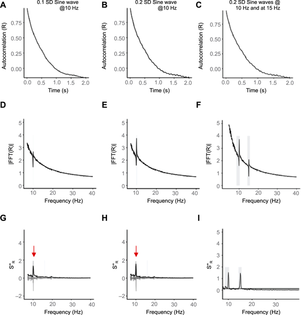
Figure 2. Extracting the alpha oscillation. (A)–(C) Autocorrelation of simulated colored noise signals with γ = ∼1.75 and embedded oscillations of 10 Hz with amplitude of 0.1 SD of the signal (panel A), 10 Hz with amplitude 0.2 SD (panel B) and 10 Hz and 15 Hz both with amplitude 0.2 SD of the signal. (D)–(F) Fast Fourier Transform (FFT) of each of the autocorrelations in A-C showing a peak at the embedded oscillation frequency of 10 Hz (D,E) or 10 Hz and 15 Hz (F). (G)–(I) Hilbert envelope (black) of the second order differential of the FFT (grey). Red arrow shows peak. The area under the Hilbert envelope that exceeds the threshold of 1 SD of the difference function is defined as the oscillation energy (here Eα since the oscillation at 10 Hz is within the alpha band).
Download figure:
Standard image High-resolution image2.2. Computing the oscillation energy
Periodicity embedded within a signal can best be visualized by looking at its autocorrelation function. Figures 2(A)–(C) show the autocorrelation for the simulated signals with varying amplitudes of the embedded sine wave (2(A), (B) power noise with γ = 1.75 and 10 Hz sine wave amplitude of 0.1SD and 0.2SD the signal amplitude; C: sine waves at 10 and 15 Hz at 0.2SD amplitude). Our method therefore involves first computing the standard autocorrelation (R) of the signal.
We next compute the fast fourier transform or FFT of the autocorrelation which provides an estimate of the power spectrum or PSD. We note that one could use any spectral transformation such including the Welch method (pwelch), the FFT2 or the autoregressive spectral analysis of the signal in its raw or pre-processed forms Fundamentally these are all intended as estimates of the power spectrum of the signal, but practically, since they are only estimates, they differ considerably due to various parameters within the algorithm such as the type of window and window overlap used. The Welch method uses greater window overlap and averaging which smooths the spectrum, broadens any peaks and also results in shallower slopes overall, while the FFT2 has more noise. Autoregressive spectral analysis is a different algorithm that is more suited for short signal lengths. These aspects are extensively discussed in signal processing textbooks so we do not address this in further detail here. We have chosen to use the FFT of the autocorrelation (R) since the autocorrelation provides an intermediate step that provides a useful visualization of the presence of periodicity. We compute this using a standard FFT function that utilizes a hanning window and represent it with the notation SR so as to distinguish from the PSD computed using other methods.

Like the PSD shown in figure 1, this produces peaks corresponding to the frequency of the embedded oscillation (figures 2(D)–(F)). However, when the amplitude of the embedded oscillation is small (for example as in 1(C)), the peak is often barely visible. Thus, to detect small oscillations the peak must be amplified.
To amplify detection of the oscillation and suppress the background decay we use a second order differential of the function. This is a method commonly used in spectroscopy and other fields to amplify the detection of small signals embedded within decaying backgrounds. The higher order the differential, the greater the amplification of small signals. Here we compute  as the second order difference function of the FFT of the autocorrelation (figures 2(G)–(I), grey line).
for which the numerical derivative is equivalent to

We then compute the Hilbert amplitude envelope (H) of this second order difference function (i.e.  (figures 2(G)–(I), black line). Essentially this represents the absolute value of the analytic function obtained by the Hilbert transform. We do this using the env function in R within the seewave package (https://cran.r-project.org/web/packages/seewave/seewave.pdf) using a mean sliding window of length 4 points and an overlap of 50% between successive windows. The length of the window is the primary determinant of the degree of smoothing of the envelope.
The next step is to identify the peaks in the envelope. To do so we use a method that deliberately avoids the use of a fixed window or range (e.g. 7.5 to 12.5 Hz for the alpha band) within which to identify peaks, since fixed windows can bias the detection and miss peaks on or outside the boundaries. Instead, we use a threshold of one standard deviation (SD) of the envelope function to identify those segments with values continuously greater than 1SD. To accomplish this all values of the envelope below the 1SD threshold are set to 0. The thresholded Hilbert envelope HT is thus

We then find the index values for the nonzero values of HT and compute the difference between successive index values. Differences greater than 1 indicate the end of one segment and start of the other. This can then be used to create vectors of the index values of HT that represent the start and end values of each segment. For example if HT = [0, 5, 7, 9, 0, 0, 6, 8, 6, 0] then the index vector IS representing the start values would be [2, 7] and the Index vector IE representing the end values would be [4, 9]. Each peak segment P1, P2, ..., Pn would thus be represented as:

We then exclude all segments that have a length or width of less than 0.1 Hz (∼12 data points) to eliminate short noise periods that are not real peaks. Each segment greater than this length cut-off is then considered a peak segment. In our simulated example the width is about 1 Hz while peaks in real EEG data typically span 2–5 Hz.
To characterize the peaks we first take each segment of the envelope that meets the above criteria and compute the maximal value to identify the peak position. The peak frequency (Pf) is then computed as the position or index on the frequency axis corresponding to the peak value shifted by two positions to the left since the envelope is computed on the second order derivative or difference function and is therefore shifted by two data points.

Where FS is the sampling rate.
We then compute the energy of the oscillation (E0) for each peak as the area under the Hilbert envelope for each segment identified above. as:

Since the embedded oscillation in our first two examples have a peak at 10 Hz which is within the alpha band, we call the computed metric Eα. In the third case the second peak is at 15 Hz (within the beta band) so is defined as Eβ.
We note that the bandpass or low pass filters applied at 1 Hz create a large peak in the power spectrum around the filter cut-off. Given this, any oscillations at frequencies less than 3 to 5 Hz are unlikely to be accurately detected as they will be indistinguishable from peaks arising from the filter as well as measurement artifacts such as baseline drifts. However, if low pass filters applied are closer to 0.1, it's possible that peaks at 1 Hz could be detected.
2.3. Sensitivity of the method
We next demonstrate the sensitivity of this measure in detecting and discerning differences in the amplitude of the embedded oscillation. In figure 3(A) we show Eα for different amplitudes of embedded 10 Hz sine waves. As can be seen, the curves are fairly similar for signals of different background decays (grey to black). Conversely, when visualized as Eα vs background decay for different amplitudes of the embedded sine wave (figure 3(B)), we see that the lines (corresponding to a particular embedded sine wave amplitude) are fairly flat allowing estimation of the embedded amplitude independent of the characteristics of the background decay
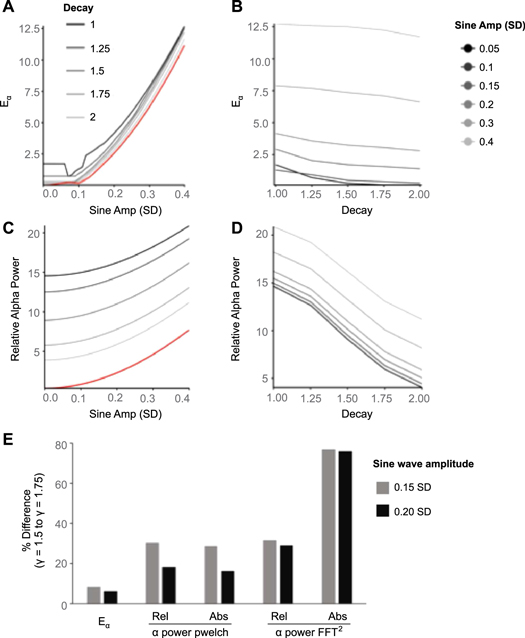
Figure 3. Sensitivity of measurement. (A) Oscillation energy (Eα) as a function of the relative amplitude of the embedded oscillation in simulated signals with different 1/fγ decays in the spectrum (γ from 1 to 2, black lines; EEG example shown in red in all graphs). (B) Eα as a function of spectral decay rate for different embedded oscillation amplitudes. Values for each amplitude are relatively stable and only slightly influenced by the decay rate. (C) Relative alpha band power computed from the power spectrum (FFT2 method, both C and D) as a function of the relative amplitude of the embedded oscillation (as in A). (D) Relative alpha power as a function of decay rate for different embedded oscillation amplitudes. Values are dominated by the decay rate and therefore insensitive to the oscillation within the range shown. (E) Change in value of estimation metric for the same amplitude of sine wave when γ changes from 1.5 to 1.75, shown as percentage. Graph compares Eα and estimations of both relative and absolute alpha power computed using different methods.
Download figure:
Standard image High-resolution imageFor comparison we show some commonly used alpha power measures (both relative and absolute from 7.5 to 12.5 Hz) computed as a function of the amplitude of the embedded oscillation for different decays, and correspondingly as a function of decay for different amplitudes (figures 3(C)–(E)). Relative power was computed as the power within the band of interest (here 7.5 to 12.5 Hz) as a fraction of the summed power across the entire computed spectrum. Figures 3(C) and (D) show the relative alpha power computed using the square of the FFT (FFT2) as a function of sine wave amplitude and 1/f decay (i.e. γ value) respectively. As can be seen, in contrast to Eα, the alpha power was more separated for each value of γ for the same sine wave amplitude (figure 3(C)) and conversely declined more substantially as a function of γ for each embedded sine wave amplitude value (figure 3(D)).
We next show in figure 3(E) how a shift in decay (i.e. γ) of the 1/f spectrum from 1.5 to 1.75 distorts the estimation of the same embedded alpha oscillation for various methods of characterization of this feature. We use percentage difference in the metric value between γ = 1.5 and 1.75 since the scales of each measure are different and show the values for two different amplitudes (0.15 and 0.2). While Eα resulted in a difference of 8% between the two decays for an amplitude of 0.15 and 6% of an amplitude of 0.2, alpha power measures resulted in differences of anywhere from 13% to 78% depending on the method used. In general, using the pwelch method resulted in less decay dependent distortion relative to using the FFT2. This is most likely due to the additional averaging of windows in the welch method which can result in broader peaks in the estimated power spectrum. Further both relative and absolute alpha power gave similar results for pwelch but relative performed better for FFT2.
Thus, studies that seek to study alpha oscillations using alpha power (relative or absolute) are prone to misinterpret changes in decay of the 1/f spectrum as changes on the alpha oscillation. Indeed alpha changes reported using power spectrum could easily arise from a small shift in the decay rather than any change in the periodicity or oscillation, particularly when the oscillations in the signal are weak. Further, these comparisons demonstrate the substantial variability in results depending on the method used for computing the alpha band power. This suggests caution in the interpretation of results using these traditional metrics.
Our measure of oscillation energy (E0) will allow researchers to detect smaller oscillations with greater sensitivity and specifically study changes in the peaks, which thus describes the oscillatory component more independent of the decay of the background envelope.
3. Application of method to real EEG examples
We next show a detailed application of this method using recordings obtained from 24 adults between the ages of 21 and 50 sitting quietly for three minutes with their eyes closed followed by three minutes with their eyes open. The recordings were obtained using the Emotiv EPOC+ with a 14 channel device (channel locations AF3, AF4, F3, F4, F7, F8, FC5, FC6, T7, T8, P7, P8, O1 and O2) with a sampling rate of 128 Hz and bandpass filtered between 1 and 50 Hz. All recordings were obtained following informed written consent using protocols approved by the Health Media Lab's Institutional Review Board (IRB #00001211, IORG #0000850) in accordance with the requirements of the US Code of Federal Regulations for the Protection of Human Subjects.
Figure 4 shows a detailed application of the methodology to examples of eyes closed recordings from one channel from each of three different subjects. Panels A-C show the autocorrelation of each record demonstrating different oscillation and background decay profiles. The first example (channel O2) shows a relatively weak oscillation with a peak at 12.43 Hz. The second example (channel O1) shows a strong oscillation with a peak at 9.42 Hz while the third example (channel FC6) shows oscillation of mixed frequencies corresponding to two peaks at 9.93 and 18 Hz. Figures 4(D)–(F) show the FFT of the autocorrelation for each example and figures 4(G)–(I) show the second order difference function and Hilbert Envelope which give rise to the Eα values of 0.46, 3.43 and 0.92 for the first peaks respectively, demonstrating a wide difference between them.
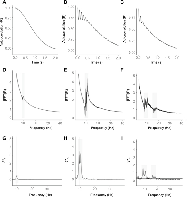
Figure 4. Oscillation parameters extracted from real EEG signals. (A)–(C) Autocorrelations of EEG signals recorded under resting eyes closed conditions from three different people shows varying oscillatory activity. A. weak oscillation B. strong oscillation C. complex oscillation (multiple frequencies) with shallower decay than A and B. (D)–(F) Spectral decomposition of the autocorrelation shows peaks corresponding to the oscillation at 12.43 Hz in panel D, 9.42 Hz in panel E and at both 9.92 Hz and 18 Hz in panel F. (G)–(I) Shows peak (vertical grey line) and area corresponding to the oscillation energy (grey shaded area under Hilbert envelope shown as black line).
Download figure:
Standard image High-resolution imageWe also point out that while the first example (4(C)) with peak of 12.43 would be considered within the alpha range, given that much of the overall peak is outside of the 12.5 Hz alpha boundary it would be partially missed by methods that use a predefined band or range and is a demonstration of the arbitrariness of the boundary definitions.
The oscillation in the autocorrelation provides the best evidence of the presence of a periodic component in the signal. However, it is important to note here that the nature of periodicity is different from that in our simulation which involves a consistent sine wave throughout the duration of the signal. Here the oscillation shows a dampening in the autocorrelation. Such a pattern most likely reflects the presence of alpha oscillations occurring in short bursts of different lengths at random intervals and is consistent with the visual pattern in the signal.
Given that the oscillation tends to occur primarily in the eyes closed state, we next show the differences between eyes closed and eyes open in Eα as well as the relative and absolute alpha power estimated using both the pwelch and FFT2 methods for each of the 24 subjects (figure 5). A histogram of the ratio of eyes closed to eyes open transformed as  is shown for each subject where 0 represents an EC/EO ratio of 1 (figures 5(A)–(C)) demonstrating that Eα was always increased in the eyes closed condition relative to the eyes open condition, indicating that there was consistently a greater peak above the background for each subject. In contrast, the absolute alpha power computed using either pwelch (figure 5(B)) or FFT2 (figure 5(C)) for the same data showed both increases and decreases that were influenced by a multitude of factors. The corresponding values for each individual subject are shown by a line joining the eyes closed and eyes open conditions for each subject (Eα figure 5(D), pwelch figure 5(E), FFT2 figure 5(F)). Overall the alpha power values had little correlation to the Eα values for the same subjects in the eyes closed condition as shown by a scatter plot of absolute alpha power values versus Eα for each individual subject (figure 5(G), r = 0.41 pwelch abs, open circles, r = 0.14 FFT2 abs, closed circles). This highlights the distinct nature of the Eα metric compared to the absolute alpha power measures.

Figure 5. Alpha oscillation peak characterization in Eyes Closed and Eyes Open Conditions. (A)–(C) Ratio of Eyes Closed (EC) and Eyes Open (EO) values for different metrics for each of 24 Subjects shown as a histogram of  , (an EC/EO ratio of 1 is a
  value of 0). Values are positive for all subjects for Eα (A) but vary as positive or negative for absolute alpha power estimation with pwelch (B) and FFT2 (C). (D)–(E) Eα (D) and absolute alpha power computed using pwelch (E) and FFT2 (F) for Eyes Open (EO) and Eyes Closed (EC) for each individual subject (each subject is one line). (G)
  values for absolute alpha power versus Eα (pwelch filled circles, FFT2 in open circles) for each subject shows little correlation (0.41 for pwelch and 0.15 for FFT2) indicating specificity of Eα measure. (H)–(I) Relative alpha power computed using pwelch (H) and FFT2 (I) for Eyes Open (EO) and Eyes Closed (EC) for each individual subject (each subject is one line).
Download figure:
Standard image High-resolution imageTwo factors contribute to this overall result. While the background decay remained the same between the eyes closed and eyes open conditions for the majority of individuals in this sample, 30 to 40% of the cases showed background decays with greater steepness in eyes closed condition depending on the spectral method used. Further, the absolute power was often different between the two conditions with overall power at all frequencies being higher in the eyes closed case in 54% of cases and lower in 24% of cases. The differences in overall power between the conditions can be eliminated by using relative alpha power, which yields substantially different results relative to absolute power (r = 0.04 and 0.1 between relative and absolute alpha power for pwelch and FFT2 respectively). However the contribution of differences in background decay continue to reflect in relative alpha power, still resulting in decreases seen when going from eyes open to eyes closed despite a higher peak in many of the cases (figures 5(H), (I)). Thus Eα more specifically and sensitively identifies even small increases in the alpha peak between the two conditions, providing more consistent results.
We also highlight a significant advantage of this method with respect to its relative insensitivity to artifacts in the data. One significant source of artifact in the EEG data is the eye blink which is prominent in the eyes open condition but not eyes closed. While many methods exist to remove the eye blink, none are perfect, and they tend to remove significant useful parts of the signal along with the eye blink that can change the overall profile considerably. Furthermore, ICA based methods, which are commonly used only work well when there are a large number of electrodes. In the example we have shown there are only 14 channels which are generally not sufficient for good ICA results—4–14 channels are now a common configuration that has advantages for larger scale studies as well as in rapid use first line clinical applications. The eye blink is largely in the low frequency range and while it may change the overall decay, since this method uses the second order differential rather than fitting a curve to the overall decay, it is far more sensitive to local rather than global differences in the decay and will not be significantly affected by distortions in the spectrum that are not in the local range of the oscillation of interest. In this example since we are looking at oscillations in the alpha band which is relatively far away in the spectrum from the distortions caused by the eye blink, Eα is not very sensitive to the eye blink. On the other hand, the eye blink would introduce significant distortions in methods that depend on curve fitting of the full range of the spectrum. This is one of the advantages of this method over subtracting curves fit to the decays. However, it is also another reason that low frequency oscillations in the range of eye blinks are difficult to identify.
4. Impact of parameter choice on outcomes
As in any algorithm, various parameter selections are made to optimize the outcome. The first aspect is the method of computing the power spectrum which has implications for the decay of the power spectrum as well as for the width of any peaks. The effects of different methods of computing the power spectrum are extensively discussed in signal processing text books so we do not address this further here. Subsequent to this step, the two primary assumptions are with respect to the smoothing parameter used to compute the Hilbert envelope of the second order derivative of the spectrum, and the threshold used to define peak segments. Both parameters serve to tune the segments identified as peaks with the aim of eliminating effects of noise fluctuations while optimizing the ability to discriminate between successive peaks that may be close together. Here we show the impact of these two parameter choices on both the simulated data as well as the eyes closed EEG recordings.
Figures 6(A), (B) show the impact of varying the smoothing factor in the computation of the Hilbert envelope in the simulated and eyes closed EEG data respectively while keeping the threshold used to define peak segments was kept constant at 1SD. The smaller the value the more the envelope will track all the small fluctuations such that one peak segment can become split into multiple segments when thresholded due to noise fluctuations, resulting in smaller Eα and potentially multiple peaks. Conversely the larger the value the more it will interpolate values to create a smoother envelope. While this can aid in more accurate peak detection, it will also particularly affect the inclusion of smaller upticks at the start and end positions of the peak segment, potentially shortening the segment considered and ultimately reducing Eα for high values. This is reflected in figure 6(A) where the maximal value of Eα occurs at a value of 4 representing an optimal value where exclusions due to noise fluctuations and segment shortening due to smoothing are minimized. A similar pattern arises in the real data (figure 6(B)), further validating the choice of smoothing parameter.

Figure 6. Impact of parameter choice on Eα estimation. (A) Effect of smoothing parameter on Eα for simulations with different decay exponents γ ranging from 1(top) to 2 (bottom). Actual EEG trace shown in red. (B) Effect of smoothing parameter on Eα for EC recordings for each of 24 subjects shows maximum at length 4. Average shown in red. (C) Effect of choice of threshold (in multiples of SD of the Hilbert envelope) on Eα estimation for simulations with different decay exponents γ ranging from 1 (top) to 2 (bottom). Actual EEG trace shown in red. (D) Effect of choice of threshold as in C for each of 24 subjects shows a drop in Eα as threshold increases to 1SD. Average shown in red.
Download figure:
Standard image High-resolution image
Figures 6(C), (D) show the impact on Eα of varying the threshold from 0.5 to 1.5 times the standard deviation or SD of the Hilbert envelope while keeping the smoothing parameter constant at 4. At lower thresholds the algorithm will increasingly group fluctuations into one large peak segment while higher thresholds will increasingly separate small fluctuations arising from noise into distinct peak segments. Thus the lower the threshold the larger Eα will be, and the higher the threshold the smaller Eα will be. Figure 6(C) shows the impact of varying the threshold on detection of the 10 Hz peak in the simulated data and 6(D) shows the impact of varying the threshold on the detection of the first peak in the eyes closed recordings for each of the 24 subjects. In the simulated data since the peaks are very sharp (many SD from the overall envelope), the impact is very small in this range. However, in the real data Eα decreases considerably as the threshold goes from 0.5 to 1 but stays relatively stable after that such that 1SD represents the minimum threshold where most of the noise is excluded.
We note here that the optimal choice of this may be specific to the FFT parameter choices used which influence the noise fluctuations in the spectrum. Further, when genuine peaks are too close together they will be impossible to resolve with certainty and will be grouped as an integrated band. We also note that the values obtained for an individual would depend on various hardware and methodological choices such as the reference selection, electrode properties, signal filtering, any preprocessing of the data such as ICA and method of computing the power spectrum or spectral density. Given the wide methodological variability in the EEG field and the challenges these pose [23], these aspects should be specified clearly when using the algorithm to allow for comparison across studies.
5. Discussion
The power spectrum of the EEG has a 1/f-like decay with occasional embedded periodicity that give rise to peaks above this 1/f decay. This periodicity or periods of regular oscillatory activity, typically at ∼10 Hz (alpha oscillations), is observed most reliably under eyes closed conditions, and is thought to have a role in attention and attention related disorders. Accurately characterizing the emergence and properties of peaks independent of the background decay may therefore provide more specific insights into its role in brain health and behavior.
5.1. Summary of method
Evidence suggests that the background 1/f signal is largely composed of complex waveforms rather than multiple independent periodic components. However, the conventional method of assessing oscillations are based on summing the power spectral density or PSD within a particular frequency band that (i) include both the oscillation and 1/f background component in estimation and (ii) using fixed frequency boundaries. Both of these aspects introduce significant error into estimation of the periodic or oscillatory component. While oscillations most frequently arise in the alpha range (7.5 to 12.5 Hz), the peak values and the width of the power spectrum that they span can vary based on both intrinsic aspects of the signal and parameter choices used in computing the PSD (e.g. window overlap). In some cases (as in the example shown in figure 4(A)), the peak may spread across two bands resulting in an underestimation when considering one band alone. Further, oscillations can arise simultaneously at multiple frequencies (i.e. two peaks) and can be missed.
Using colored noise simulations as well as an example of a real EEG signal embedded with either a single 10 Hz sine wave or multiple sine waves at 10 and 15 Hz, we have defined a method to characterize multiple peaks emerging from embedded oscillations in a manner that is relatively independent of the nonperiodic background spectral envelope. We have termed this measure Oscillation Energy, to distinguish it from power, and abbreviated to E0, it provides an aggregate measure of the strength and fidelity of the oscillation. Our measure is less sensitive to changes in the 1/f decay of the overall spectrum and therefore performs better than the traditionally used estimations of power within any a spectral band such that differences between individuals or conditions can be more directly attributed to the periodic component. Further, since it amplifies the peaks it has a higher sensitivity to smaller peaks relative to other methods to separate out the peak [21]. We use Eα to indicate the energy of the oscillation whose peak is detected within the alpha band, Eβ to indicate the energy of the oscillation in the beta band and so on.
The fundamental premise of this method rests on the property of derivatives of peak-like signals whereby the amplitude of the nth derivative is inversely proportional to the nth power of the width of the peak (for a peak of the same shape and amplitude). Consequently, when a peak arises out of a slower decaying background, representing a relatively narrow period of faster change, each higher order derivative will amplify the peak while suppressing the background which is effectively a stronger but broad peak.
The key advantage of this measure is that it specifically amplifies the periodicity and minimizes the impact of the decay of the PSD, allowing both identification of the presence of small oscillations as well as greater discrimination of specific differences in the oscillatory component. It is also aided by defining the period of interest based on a threshold rather than by an arbitrary frequency range, and therefore provides a 'band' independent metric. Since the second derivative with respect to a position is acceleration or momentum, the nomenclature of energy might be thought of in terms of its relation to the momentum with which the oscillation exceeds the background.
We do note however that the method does have some limitations in that it amplifies differences in a nonlinear manner and also cannot fully eliminate the impact of background decay. It therefore does not allow for a specific estimate of the oscillation amplitude. Second, while the evidence suggests that the background spectral decay is largely composed of nonperiodic waveforms, this may not always be the case. Third, very broad peaks and peaks close to the resolution of the power spectrum cannot be easily detected, making it a challenge to detect low frequency peaks arising at less than 1 Hz. Finally, the signal is non stationary and peaks that arise may not always reflect periodic activity. Therefore, a more generalizable interpretation of this measure would be the degree to which any peak exceeds the overall background activity, analogous to a signal to noise measure.
Finally, we note that the metric is impacted by several parameter choices such as the window type and overlap used in the FFT computation as well as the smoothing parameter of the Hilbert transform and the threshold of the Hilbert envelope used to define the peak segments and therefore oscillation energy. Consequently, unless the parameters used are identical (as is the case for other measures such as the power as well), the absolute values will not be informative. Rather this serves more as a relative measure to compare across two records.
In conclusion, E0 provides a more precise metric for periodicity that will enable researchers in the field to develop a clearer understanding of the function of this feature of the signal. In this context, it could ultimately prove to be useful in understanding and predicting behaviors that rely on this feature. For example, attention has been shown to have a relationship already to the overall power in the alpha band [24, 25], although at low correlation levels, which possibly could be improved by use of this metric alone or in combination with overall alpha band activity. Further, since it is not yet known which features of the EEG signal, alone or in combination, are fundamentally important to each different behavior or outcome, there is a need in the field to explore many different features. For example, features of the EEG such as different frequency bands generally have on average 0.3 to 0.4 correlations with different mental health or behavioral outcomes [23]. Features extracted by this algorithm represents a new dimension that may be better able to predict different outcomes than other methods, or even perform better for some outcomes over others, eventually finding application in various areas.