
Abstract
Fracture toughness, as a crucial mechanical property, is essential in the research of fatigue crack propagation and fatigue life. Considering the enormous data scatter of the fracture toughness in experiments, a data processing method is proposed to calculate the fracture toughness for the specified reliability. Based on the traditional data processing method shown in the relative standards, the two-dimensional, one-sided tolerance factor is introduced to calculate the influence of the reliability. In addition, by comparing the data processing methods of the fracture toughness presented in the ISO12135:2016 and ASTM E1820-2013 standards, the differences between them were mainly the range of the qualified data, the function of the construction line, and the equation of the regression line. Because the construction lines of the two standards are based on two different material constitutive models, if the constitutive model of material is more aligned with that of the ideal elastic plastic material, the ASTM E1820-2013 standard is recommended; otherwise, the ISO12135:2016 standard is recommended. For 30CrNi2MoVA, the ISO 12135:2016 standard was more suitable, and the error of the JIC obtained by the two standards was about 5%.
Export citation and abstract BibTeX RIS

Original content from this work may be used under the terms of the Creative Commons Attribution 4.0 licence. Any further distribution of this work must maintain attribution to the author(s) and the title of the work, journal citation and DOI.
1. Introduction
The fracture toughness, as one of the most important mechanical properties, indicates a material's resistance to crack propagation. It is used widely in the structural design and fatigue life predictions of structures with defects [1, 2]. An accurate and reliable determination of the fracture toughness is of great importance for the failure assessment of equipment.
At present, the fracture toughness tests are performed mainly following the ISO 12135:2016 and ASTM E1820-2013 standards, which are the most accurate methods for measuring the fracture toughness [3, 4]. For different materials and working conditions, different kinds of specimens and experimental procedures have been proposed in the literature to measure the fracture toughness. In 1981, the small punch (SP) technique was proposed for radiation embrittlement studies in the United States. This technique was extensively developed by many researchers to estimate the potential for residual life assessment of components during service [5–8]. The Charpy impact test was proposed to avoid the disadvantages of traditional CT(Compact Tension) and SENB(Single Edge Notch Beam) samples. In contrast, this test requires smaller specimens and simpler experimental equipment. However, its result only shows the susceptibility of steel to brittle fractures instead of providing the value of fracture toughness [9]. Chen et al. proposed a method to accurately estimate the fracture toughness for 16MnDR steel in the transition region under different test conditions using the master curve method [1, 10]. The cracked Brazilian disk (BD) method was proposed by Atkinson to calculate the fracture toughness data for brittle materials [11]. The spherical indentation test (SIT) was proposed to measure the fracture toughness for ductile metals [2]. Jelitto et al proposed an experimental method to measure the fracture toughness values of porous materials. However, the CT and three-point bending specimens are the two most common specimens [12]. In particular, CT samples require smaller dimensions and are more suitable for tests of high fracture toughness values.
However, due to defects in the material itself and randomness during the sample processing and experimental loading, even though the experiment process is strictly followed and controlled according to the experiment standard, the test results of the fracture toughness inevitably exhibit considerable statistical dispersion [13]. With the development of a reliable design, the influence of the uncertainties has attracted growing amounts of attention of researchers [14]. The scattered behavior of the fracture toughness of fiber-reinforced hybrid bio-composites has been investigated in detail by Chandramohan et al. [15, 16]. Tagawa et al. researched the in the ductile–brittle transition of a structural steel, and the Weibull distribution was applied to describe the scatter characteristics of the fracture toughness [17, 18]. Lia and Zhou proposed a modified analytical model of the fracture toughness of composite materials, which allowed the possible range of fracture toughness values to be predicted as a function of the microstructure [19]. Wallin proposed a new statistical assessment method to analyze the Euro fracture toughness data set, and the results could be used to form a new basis for the micro-mechanistic modelling of cleavage fracture [20]. Xu et al proposed a method to calculate the scatter of the fracture toughness using the normal function. However, this method was not able to account for historical data, and a vast amount of data were required [21].
Although many studies have examined the reliability and scatter of fracture toughness, the studies on how to obtain the fracture toughness with a specified reliability are rare. However, in the design of the structural damage tolerance considering the reliability, this parameter is necessary. Generally, a high reliability of the fracture toughness cannot be obtained without a large number of samples and tests. Herein, a method to obtain the value of the fracture toughness with a specific reliability is proposed by introducing a two-dimensional one-sided tolerance factor.
Tests of the fracture toughness can be divided into two types: tests on linearly elastic materials and tests on elastoplastic materials. The former is usually used for brittle materials, and for highly ductile metal materials, such as those used in pressure vessels, the latter test is more suitable. The fracture toughness is usually characterized by the J-integral. Because the material tested in this study is used for high-pressure vessels, the elastoplastic fracture toughness JIC is more reasonable.
The outline of this article is as follows: In the 'Materials and Methods' section, the basic material properties and test procedure for the fracture toughness are presented, and the J-Δa data set of four specimens was obtained. Data processing was conducted following the ISO 12135:2016 standard, and the reliability was considered. A method to calculate the fracture toughness JIC at the specified reliability is proposed. Furthermore, a comparison between the JIC values obtained by the ASTM E1820-18ae1 and ISO 12135:2016 methods was performed and discussed. Finally, conclusions are presented.
2. Materials and methods
2.1. Material properties
The material tested in this study was 30CrNi2MoVA, a high-strength steel alloy. The main components, heat treatment process, and basic mechanical property are presented in the table 1–3, respectively [22].
Table 1. Components of 30CrNi2MoVA.
| Elements | C | Mn | P | S | Si |
|---|---|---|---|---|---|
| Content | 0.28–0.35 | 0.40–0.80 | ≤0.015 | ≤0.015 | 0.20–0.35 |
| Elements | Cr | Ni | Mo | V | Cu |
| Content | 0.80–1.15 | 2.00–2.50 | 0.30–0.40 | 0.15–0.20 | <0.20 |
Table 2. Heat treatment process of 30CrNi2MoVA.
| Mean temperature (°C) | Soaking time (h) | Hardening temperature (°C) | Holding time (h) | Cooling type |
|---|---|---|---|---|
| 550 ± 10 | 2–3 | 870 ± 10 | 5–6 | oil cooling |
| Mean temperature (°C) | Soaking time (h) | Tempering temperature (°C) | Holding time (h) | Cooling Type |
| 350 ± 10 | 2–3 | 600–640 | 8–10 | oil cooling |
Table 3. Basic mechanical performance of 30CrNi2MoVA.
| Mechanical Performance | σb (MPa) | σs (MPa) | Elasticity modulus (GPa) | Poisson's ratio |
|---|---|---|---|---|
| 30CrNi2MoVA | 978.14 | 893.24 | 210 | 0.21 |
2.2. Test of fracture toughness JIC
2.2.1. Specimen preparation
For stable crack growth, the J-Δa curve is generally used to describe the ability of the material to resist the crack extension, and it is also called the J − R resistance curve or J-R curve. The critical J-integral, JIC, at the onset of cleavage fracture is considered to be the fracture toughness, and it is a point on the J − R curve. The J-Δa curve is the foundation of the test of the fracture toughness, JIC. In this study, JIC was obtained by a single sample method. Namely, one whole J-Δa curve can be obtained by one specimen. To improve the reliability of the test results, four sets of J-Δa curves were obtained using four specimens.
As shown in figure 1, a CT specimen was used in the test, and the processed specimen is shown in figure 2. Their specific dimensions are shown in table 4.
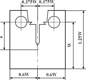
Figure 1. Standard CT Sample.
Download figure:
Standard image High-resolution image
Figure 2. Processed Specimen.
Download figure:
Standard image High-resolution imageTable 4. Dimensions of Specimens for JIC Test.
| BAVE (mm) | WAVE (mm) | BN (mm) | a0 (mm) | W-a0 (mm) | |
|---|---|---|---|---|---|
| J-01 | 10.12 | 40.00 | 8.08 | 22.22 | 17.78 |
| J-02 | 10.20 | 40.02 | 7.98 | 22.24 | 17.78 |
| J-03 | 10.22 | 40.16 | 8.02 | 21.70 | 18.46 |
| J-04 | 10.18 | 40.11 | 8.01 | 22.50 | 17.61 |
2.2.2. Test procedure
The test was conducted strictly following the standard, and the test procedure can be divided into four stages: (1) fatigue pre-cracking procedure, (2) side grooves, (3) loading and testing, and (4) data recording and analysis.
The main machine and gauge involved in this test are shown in figure 3.
- (1)The fatigue pre-cracking was conducted under a controlled force. The load type was a sinusoidal cyclic load with a stress amplitude of 10.00 kN and stress ratio of 0.1. As the crack grew, the stress amplitude gradually decreased. However, over the entire loading procedure, the loading amplitude was less than 1 kN.
- (2)In the test of JIC, side grooves are highly recommended when the compliance method of the crack length prediction is used. The side grooves also ensure that a straight crack front can form. The specimens with side grooves are shown in figure 4. They are marked as J-01, J-02, J-03, and J-04.

Figure 3. Key Experimental Equipment.
Download figure:
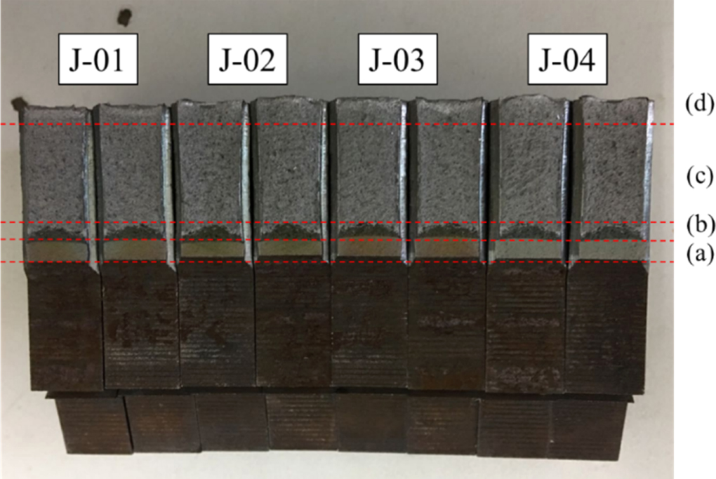
Standard image High-resolution imageIn the test of the J-Δa curve, the specimen should be broken by tension using the fatigue machine after finishing the loading. A fracture surface examination was conducted to determine the initial crack length a0 and the stable crack growth length Δa during the testing process. The macro-fracture of the broken specimen is shown in figure 5.
The macrofracture of the broken specimen can be divided into four zones: (a) Fatigue crack growing zone. In this zone, the fracture surface was smooth and flat. It was mainly produced in the fatigue pre-cracking stage. (b) Stretch zone. The front of the zone was arch shaped, and it was mainly formed during the crack initiation stage. (3) Stable crack zone. This zone was produced during the stable crack propagation stage under the effect of stable cyclic loading. (4) Final fracture zone. This zone was formed in the last tension broken stage of the experiment, and the surface of this zone was very coarse.

Figure 4. JIc Specimens with side grooves.
Download figure:
Standard image High-resolution image2.2.3. Test results
The Δa and J data of the four specimens were calculated and recorded by the gauges automatically. J-Δa curves of the specimens are shown in the figure 6 and are distinguished using different marker shapes.

Figure 5. Macrofracture of broken specimen.
Download figure:
Standard image High-resolution imageAs mentioned above, the ISO 12135:2016 and ASTM E1820-18ae1 standards are the two most common methods for testing the material fracture toughness. They involve similar experimental processes to obtain the J-Δa data but have a few differences in the data processing procedure. Thus, in the next section, the data processing procedure of the fracture toughness is performed using the two standards.
3. Data processing considering the data reliability (ISO 12135:2016)
In the ISO 12135:2016 standard, a data processing method is provided. The data for a crack extension with Δa > 0.1 is used to calculate the JIC and is fit by the following equation:

where α, C1 ≥ 0, and 0 ≤ C2 ≤ 1.
During the data fitting process, it was found that the value of α was close to zero, so its value was set to α = 0 for fitting convenience. Finally, the fitting results of the four specimens are shown in table 5. Their fitting curves are shown in figure 6 and expressed by the different line types. Figure 6 shows that the J-Δa curves of the four specimens had the same variation trend. However, for the different specimens, there were subtle differences between the J-Δa curves. This mainly resulted from the differences in the material microstructure, processing technology, and heat treatment process. Generally, the average fracture toughness values of the different specimens are determined to be the final measured values. However, with the wide application of the reliability design method, it would be better if the highly reliable fatigue fracture parameters could be used in the damage tolerance design and the fatigue life prediction. Thus, in this study, the two-dimensional, one-sided tolerance factor was used to obtain a J-Δa curve considering the reliability. It is marked as the p-γ-J-Δa curve.
Table 5. Test Results of Specimens.
| Specimens number | C1 | C2 | Correlation coefficient | J-Δa equation (J-Δa)) | |
|---|---|---|---|---|---|
| ISO 12135:2016 | J01 | 189.79 | 0.2095 | 0.9941 | J = 189.79 × Δa0.2095 |
| J02 | 189.82 | 0.2334 | 0.9987 | J = 189.82 × Δa0.2334 | |
| J03 | 208.94 | 0.2497 | 0.9965 | J = 208.94 × Δa0.2497 | |
| J04 | 197.95 | 0.2073 | 0.9972 | J = 197.95 × Δa0.2073 | |
| ASTM E1820-18ae1 | J01 | 189.5605 | 0.1838 | 0.9999 | J = 189.5605 × Δa0.1838 |
| J02 | 192.6129 | 0.2313 | 0.9999 | J = 192.6129 × Δa0.2313 | |
| J03 | 212.6935 | 0.2589 | 0.9999 | J = 212.6935 × Δa0.2589 | |
| J04 | 199.7925 | 0.2035 | 0.9999 | J = 199.7925 × Δa0.2035 |

Figure 6. J-Δa Curves of specimens.
Download figure:
Standard image High-resolution imageStatistical data has shown that the dispersion of the fracture toughness is greater than that of the other mechanical property parameters. The fracture toughness approximately follows the three-parameter Weibull distribution, lognormal distribution, and normal distribution [13]. The Weibull distribution is usually applied in studies of the relationship between the fracture toughness and temperature. With fewer specimens, it is difficult to accurately estimate the three parameters of the Weibull distribution. According to the research of Liu and Xiong, the lg(J)-(Δa) data follows a normal distribution [23, 24], which can be expressed as follows:

Taking the logarithm of both sides of equation (1) yields the following:

Letting y = lg(J), x = lg(Δa), β0 = lg(β), and β1 = γ0, equation (2) is transformed into the following:

As equation (3) shows, y is linearly related to x. As lg(J) follows a normal distribution, when the reliability is p, lg(J) can be expressed as follows:

where yp is the value of lg(J) when the reliability is p, and up is the p quantile of the standard normal distribution, i.e.,

The value of up can be determined using the normal distribution table. However, the true value of [lg(J)]p cannot be obtained in practice. Hence, the upper and lower confidence limits of [lg(J)]p are usually applied in the reliability analysis. In this study, a conservative value of the fracture toughness was sought, so the lower confidence limit of [lg(J)]p was used, denoted as [lg(J)]pl.
The sample average  and sample variance S2 are the unbiased estimators of population mean μ0 and population variance σ2, respectively. [lg(J)]pl with a confidence coefficient γ can be expressed as follows:

and thus,

where k is the two-dimensional, one-sided tolerance factor. It is calculated as follows:


where uγ is a quantile of the standard normal distribution, n is the degree of the sample mean  and f is the degree of sample variance S2.
  and S2 may come from different samples, so there is no certain relationship between f and n. When
  and S2 come from the same sample, f = n − 1. In this case, k is transformed into a one-dimensional, one-sided tolerance factor. If k is determined, then [lg(J)]pl can be calculated using equation (6). The lower confidence limit of the J-Δa curve with the given reliability p and confidence coefficient γ can be obtained.
In this study, four sets of experimental data were obtained, namely n = 4 and f = 3. Substituting the given reliability p and confidence coefficient γ into equation (8), the value of k can be obtained. According to equation (6), the key for the calculation of [lg(J)]pl lies in the calculation of  and S2. For the four specimens, the crack extension Δa recorded during the experiment process was not always the same. To obtain the value of lg(J) corresponding to the different crack extensions Δa of the different specimens, the change range of Δa was set to 0.1–1.6 mm. For a given crack extension Δa, the corresponding value lg(J) of the specific specimen is marked as lg(J)ji. It is calculated as follows:

where, j is the number of the specimens (e.g., 1,2,3, or 4), and i is the data point corresponding to the crack extension Δa. For every data point, the relative sample average  and sample variance Si2 can be calculated as follows:


Substituting equations (11) and (12) into equation (6), the lower confidence limit [lg(J)]pli corresponding to the relative data point can be obtained. The [lg(J)]pli are fit, and the p-γ-J-Δa curve of the material can be obtained. Here, p = 95%, γ = 95% and p = 99%, γ = 95% were considered. In addition, the average J-Δa curve of the four specimens was also calculated for comparison. The curves are shown in figure 7, and their corresponding J-Δa equations are presented in table 6.
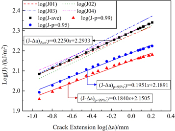
Figure 7. lg(J)-log(Δa) curve considering the reliability (ISO 12135:2016)
Download figure:
Standard image High-resolution imageTable 6. J-Δa Equations for different reliabilities.
| ISO | ASTM | |||
|---|---|---|---|---|
| Reliability | Correlation coefficient | J-Δa equation (J-Δa)p(ISO) | Correlation coefficient | J-Δa equation (J-Δa)p(ASTM) |
| ave | 1 | (J)ave = 196.4717 × Δa0.2250 | 1 | (J)ave = 198.2011 × Δa0.2208 |
| p = 95%, γ = 95% | 0.9925 | (J)p=95% = 154.5610 × Δa0.1951 | 0.9999 | (J)p=95% = 151.4167 × Δa0.1608 |
| p = 99%, γ = 95% | 0.9842 | (J)p=99% = 141.4165 × Δa0.1840 | 0.9999 | (J)p=99% = 136.9973 × Δa0.1391 |
As shown in figure 7, the solid line with the rectangle markers represents the average J-Δa curve of the four specimens, which is marked as (J-Δa)ave. The solid line with the circle markers represents the J-Δa curve when the reliability p = 95%, which is marked as (J-Δa)p=95%. The (J-Δa)p=99% corresponding to a reliability of p = 99% is shown by the solid line with triangle markers. When the crack extension Δa was the same, (J)ave > (J)p=95% > (J)p=99%. This means the if the data reliability is taken into consideration, the fracture toughness JIC obtained from the J resistance curve is smaller, and a more conservative result is obtained.
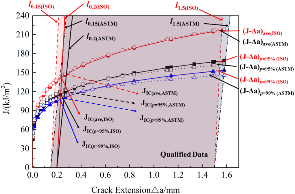
Next, according to the ISO 12135:2016 standard, J versus Δa is plotted in figure 8 and expressed by the solid line with solid symbols. For this standard, the construction line was determined based on that the material's true stress–strain relationship satisfies a power law [25]. The construction can be expressed as follows:

where Rm is the ultimate tensile strength in MPa.

Figure 8. Fracture toughness JIC of the samples when p = 0.5, 0.95, and 0.99 (ISO and ASTM).
Download figure:
Standard image High-resolution imageAs shown in figure 8, the black straight line is the construction line. The data located in the zone marked by red is the qualified data. The left and right boundaries of the qualified data region are shown by lines parallel to the construction line intersecting the abscissa at 0.15 and 1.5 mm, respectively. They are marked as l0.15(ISO) and l0.5(ISO), respectively. A line parallel to the construction and exclusion lines is plotted at an offset value of 0.2 mm. It was marked as l0.2(ISO), and its equation can be expressed as follows:

The intersection of the line l0.2(ISO) and the J-Δa curve is defined as J0.2BL, which can be calculated by solving equations (6) and (14). However, the validity must be judged in accordance with the ISO 12135:2016 7.6.2.3, 7.6.2.4, and 7.6.2.5 (ASTM E1820-2013 A9.8 Qualification of Data) standards. The results show that the values of J0.2BL with different reliabilities all satisfied the requirements of this standard. As the J0.2BL is independent of the dimensions of the specimens, in engineering applications, it is usually taken as JIC. The JIC value determined while considering the reliability is marked as JIC,p as shown in table 7.
Table 7. Value of JIC for three different reliabilities.
| ISO | ASTM | |||||
|---|---|---|---|---|---|---|
| Materials | Reliability | ΔaIC/mm | JIC/kJ · m−2 | ΔaIC/mm | JIC/kJ · m−2 | Error |
| 30CrNi2MoVA | ave | 0.2427 | 142.8633 | 0.2802 | 150.1325 | 5.09% |
| p = 95%, γ = 95% | 0.2348 | 116.4972 | 0.2653 | 122.3288 | 5.01% | |
| p = 99%, γ = 95% | 0.2323 | 108.1046 | 0.2606 | 113.6166 | 5.10% | |
| APL 5 L X80 | ave | 0.3110 | 250.2218 | 0.4177 | 279.3256 | 11.63% |
| p = 95%, γ = 95% | 0.2374 | 85.2881 | 0.2722 | 92.0648 | 7.95% | |
| p = 99%, γ = 95% | 0.2252 | 57.5140 | 0.2479 | 61.0829 | 6.21% | |
| Alloy6061-T6511 | ave | 0.2183 | 23.2120 | 0.2402 | 24.7391 | 6.70% |
| p = 95%, γ = 95% | 0.2128 | 16.2866 | 0.2276 | 17.0254 | 4.58% | |
| p = 99%, γ = 95% | 0.2105 | 13.3992 | 0.2221 | 13.6714 | 3.71% | |
| Ductile Cast Iron | ave | 0.2458 | 65.7805 | 0.2522 | 71.2061 | 8.25% |
| p = 95%, γ = 95% | 0.2320 | 46.0171 | 0.2365 | 49.9095 | 8.46% | |
| p = 99%, γ = 95% | 0.2268 | 38.6217 | 0.2306 | 41.9487 | 8.61% | |
4. Data processing considering the data reliability (ISO 12135:2016)
4.1. Comparison on the J resistance curves
In addition to the ISO 12135:2016 standard, the ASTM E1820-18ae1 standard is also a standard for the testing of the fracture toughness. They are similar, but there are differences in the data processing procedures. Guan and Li presented a comparison on these test methods [25]. However, the comparison was performed on different samples. The data scatter of the fracture toughness likely increased the differences between the results obtained by the two standards. Thus, in this paper, the comparison was conducted using the same sample to avoid the influence of randomness.
In the ASTM E1820-18ae1 standard, the construction line is determined based on the assumption of the elastic–perfectly plastic material [25]. It is expressed as follows:

where M ≥ 2, and it can be determined from the (J, Δa) data as well. Here, M = 2. σY is the effective yield strength, which is an assumed value of the uniaxial yield strength. It can be calculated as follows:

where σYS is the 0.2% offset yield strength, and σTS is the ultimate tensile strength.
The qualified data region in the ASTM E1820-18ae1 standard is confined by Jlimit, ∆amin, and ∆alimit. Jlimit can be calculated as follows:

Two parallel lines with an offset of 0.15 and 1.5 mm from the construction line were plotted and marked as l0.15 and l1.5, respectively, as shown in figure 9. They are plotted as two red solid lines.

Figure 9. J-Δa curves of specimens.
Download figure:
Standard image High-resolution image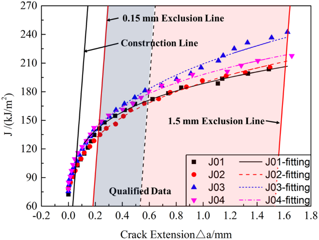
Then, similar to the ISO 12135:2016 standard, the data that fell in the region between the l0.15 and l1.5 were used to determine a linear regression line of the following form:

If k = 1.0 mm and α in equation (1) is 0, equation (19) can be transformed into equation (1). However, for the two standards, the data used to fit the regression line were slightly different, so the regression line was slightly different. For the ASTM standard, the regression lines of the specimens were expressed by different types of lines, and their corresponding equations are shown in table 5.
As shown in table 5, the J-Δa equations of the same sample obtained by the two standards were different. As the ASTM had higher refinements on the qualified data, the J-Δa curves of the specimens obtained by the ASTM were below those obtained by the ISO. However, this does not indicate that the material fracture toughness JIC obtained by the ASTM is more conservation, because the value of the fracture toughness JIC is decided by the regression and construction lines. The construction line in the ISO standard has a bigger slope and influences the value of JIC as well.
4.2. Comparison of J resistance curves considering the reliability
A similar method to that used in the section 3 is applied in this part. The J-Δa curves for different reliabilities were obtained as shown in figure 8. They are expressed by the dashed line with hollow symbols. In the ASTM standard, the qualified data are limited to the region confined by the l0.15(ASTM) and l1.5(ASTM), which are expressed by the black dashed–dotted lines in this figure.
As shown in the figure, the average J-Δa curves obtained by the different standards almost coincided, while the J-Δa curves considering the reliability were slightly different. When the crack extension was very small, the (J-Δa)p(ISO) and (J-Δa)p(ASTM) were slightly different. As the crack extension Δa increased, when the crack extension Δa > 0.6 mm, the differences between (J-Δa)p(ISO) and (J-Δa)p(ASTM) gradually increased.
This was mainly because the average J-Δa curve was the average value of four specimens without considering the influence of the sample variance S2. The average values of  obtained by the different standards were almost the same.
Because the J resistance equations obtained using the two standards were different, the sample variances calculated by the J resistance equations were different as well. Therefore, when the reliability was taken into account, the (J-Δa)p curves obtained by the two standards were different. As the crack extension Δa increased, the differences between the value of J obtained by the two types of J resistance equations increased exponentially. The differences shown in figure 8 are increasingly evident.
Similar to the ISO 12135:2016 standard, based on the equation of (J-Δa)p(ASTM), the material fracture toughness JIC can also be obtained by the ASTM. The result was also validated by the requirement described in the ASTM E1820-2013 A9.8 Qualification of Data standard. The values of JIC obtained by the different standards are shown in table 7. The value of ΔaIC is the crack extension length corresponding to JIC in figure 8.
As shown in table 7, the value of the fracture toughness JIC obtained by the ASTM standard was always larger than the corresponding value obtained by the ISO 12135:2016 standard. Because the construction lines of the two standards are based on two different material constitutive models, if the material constitutive model is more aligned with the stress–strain curve of the ideal elastic plastic material, the standard ASTM is recommended; otherwise the ISO is recommended. For 30CrNi2MoVA, the true stress–strain relationship was more aligned with a power function, and the the ISO 12135:2016 standard calculation of the fracture toughness was more suitable. Compared with the standard ASTM, this is a more conservative result, and the error of the fracture toughness JIC obtained by the two standards was about 5%. However, for the different reliabilities, the change of the error is subtle.
In addition to the material 30CrNi2MoVA, the calculation method on the fracture toughness of specific reliability is applied into three more other materials, and the results are shown in table7. The J-Δa data of these materials are respectively derived from the refrence [26–28]. As shown in table 7, the fracture toughness JIC obtained by the ISO standard is usually smaller than that obtained by the ASTM standard. Similar to the material 30CrNi2MoVA, the constitutive model of Alloy6061-T6511 and Ductile Cast Iron are not the ideal elastic plastic material. For them, the ISO standard is recommended. But for the material APL 5 L X80, the ASTM standard is more suitable. As described in table 7, the error of the fracture toughness measured by the two standards can even reach up to 11.63%.That means for different materials, reasonable choices of the test standard are of great importance.
For 30CrNi2MoVA and Ductile Cast Iron, the change of the error between the different reliabilities is subtle. But for the other two materials, APL 5 L X80 and Alloy6061-T6511, the change of the error is great. It is mainly related with the degree of the dispersion of the J-Δa data. For different specimens used in the test of one material, the greater are the differences between the data of different samples, the larger is the value of the sample variance S2, then the smaller is the sample average  calculated by equation (6), and more significant are the differences between the fracture toughness JIC of different specific reliability. That means, higher scatter of the experimental data is supposed to generate a more conservative fracture toughness of the specific reliability obtained by this method.
5. Conclusions
Fracture toughness, as a crucial parameter, is used widely in the research of fatigue life predictions and failure analysis. The test of the fracture toughness is one of the most common actions in such research. Because of the randomness in the test, the fracture toughness JIC considering the reliability was studied. In addition, the JIC values obtained by the standard ISO and ASTM were compared:
- (1)A new data processing method for the fracture toughness considering the reliability was proposed. The two-dimensional, one-side tolerance factor was applied to calculate the JIC for a given reliability. This method can take advantage of the current test data and historical data to decide the JIC,p value and can reduce experimental costs. By taking the reliability of the fracture toughness JIC into the account, a more conservative result was obtained, and a more reliable guarantee of the performance of the equipment was provided.
- (2)Based on the comparison of the data processing method for the fracture toughness, JIC, presented in the ISO and ASTM standards, their differences were mainly due to the range of qualified data, function of the construction line, and equation of the regression line. These differences resulted in different fracture toughness, JIC, values using the two standards, and the JIC tested by the ISO was smaller. Because the construction lines of the two standards are based on two different material constitutive models, if the material constitutive model is more aligned with the stress–strain curve of the ideal elastic plastic material, the ASTM standard is recommended; otherwise the ISO standard is recommended. For 30CrNi2MoVA, the true stress–strain relationship is more aligned with a power function, and the ISO 12135:2016 standard calculation of the fracture toughness is more suitable. For different materials, the change of the error between the different reliabilities is mainly related with the degree of the dispersion of the J-Δa data. The higher is the scatter degree of the experimental data, a more conservative value of the fracture toughness of specific reliability can be obtained by this method.
Funding
The authors disclose the receipt of the following financial support for the research, authorship, and/or publication of this article. The financial support for this work was provided by National Natural Science Foundation of China (No. 51674040), State Key Science and Technology Projects (No. 2016ZX05038-001-LH002), and the Hubei Province Natural Science Foundation (2016CFC740).
Conflicts of interest
The authors declare no conflict of interest.