
Abstract
The formation of nanoscale droplets/bubbles from a metastable bulk phase is still connected to many unresolved scientific questions. In this work we analyze the stability of multicomponent liquid droplets and bubbles in closed Nj, V, T systems (total mass of components, total volume and temperature). To investigate this problem, square gradient theory combined with an accurate equation of state is used. We compare the results from the square gradient model to the macroscopic capillary description. We find that both predict a finite threshold size for droplets/bubbles. The work reveals a metastable region close to the minimal droplet/bubble radius. We find that the liquid compressibility is crucial for the existence of this minimum threshold size for bubble formation.
Export citation and abstract BibTeX RIS

Content from this work may be used under the terms of the Creative Commons Attribution 3.0 licence. Any further distribution of this work must maintain attribution to the author(s) and the title of the work, journal citation and DOI.
1. Introduction
For nanoscale bubbles or droplets, the thickness of the interface can be of the same order of magnitude as their size. Models which do not specifically take into account surface gradients, such as classical nucleation theory and discontinuous excess formulations, might then be insufficient. We will thus use a square gradient theory for curved systems coupled with an accurate cubic equation of state [1, 2] to investigate the system. In the square gradient theory, the Helmholtz energy density has contributions up to second order in the gradients of the densities. The functional minimization of the total Helmholtz energy keeping Ni and T constant, gives the equilibrium density and concentration distributions in the canonical ensemble [3]. The advantage of this approach is that continuous profiles across the interface can be found. Square gradient theory combined with an accurate equation of state and suitable models for the pure components has been used to reproduce experimental results for the surface tension of planar interfaces of multicomponent mixtures [4]. We will use it here to describe the formation of bubbles and liquid droplets. To give further insight into how the size of the system and the composition of the fluid affect the formation of small bubbles and drops, we will compare the results to a macroscopic capillary description [5]. While previous work on this topic has focused on single-component systems [6] we formulate our problem for mixtures. In addition we give a detailed thermodynamic stability analysis.
The paper is structured as follows. First, a short introduction will be given to the use of a cubic equation of state coupled with either the square gradient theory (mesoscopic approach), or the capillary approach (macroscopic approach) to describe the formation of bubbles and droplets. We then show that the capillary approach is able to reproduce results from the square gradient theory remarkably well for a binary mixture, using hexane–cyclohexane as an example. Both approaches will be used to analyze the stability of small bubbles and the existence of a threshold size below which no stable bubbles can be formed. Finally, some concluding remarks are provided.
2. Theory
Consider a spherical container with volume V, temperature T and a fixed number Ni of moles of each component i. We assume that a perfectly spherical bubble or droplet is placed at the center of the container. We use the Peng–Robinson cubic equation of state for the pressure
where Rg is the universal gas constant, ν is the molar volume, and a,α and b are parameters of the equation of state. Furthermore  and
and  . Integration with respect to the volume gives the residual Helmholtz energy density (i.e. the difference between the Helmholtz energy of the homogeneous phase and that of an ideal gas)
The Helmholtz energy can be differentiated to give the other thermodynamic variables. A complete thermodynamic description of the system is then obtained by linking these variables to the properties of the ideal gas.
The square gradient model is a formalism frequently used to describe the surface between two phases. The equilibrium molar density distributions ci give a minimum of the Helmholtz energy functional
The subscript sgm refers to the square gradient model, κij is symmetric and will be taken constant, c will be used as short notation for the set  . The total mass of each component is specified as integral constraints:
  . We know from variational calculus that such a minimum is an extremum of a modified functional which can be interpreted as the grand potential

where μsgm,i is the chemical potential of component i. The Euler–Lagrange equations with integral constraints require that the first variation of Ω is zero, which gives, using spherically symmetry
We use as mixing rule for the square gradient constants  , where κi are the square gradient coefficients used for the description of a fluid with only component i. We define
where b labels the most abundant component. Upon substitution of these definitions, the system of differential equations reduces to one differential equation and Nc − 1 algebraic equations:

Note that  b = 1, see [3] for further details. The combined system of differential and algebraic equations was solved using the 'bvp4c' solver in Matlab. The derivatives of q were taken zero in r = 0 and at the outer boundary. The densities were scaled with the density of the liquid-phase at the bubble-point, cmax = 8.36 kmol m−3.
Following previous work [5, 7] on small bubbles and droplets we use the capillary model, to be able to compare the square gradient model to a macroscopic approach. In this model the bubble/droplet as well as the exterior phase have homogeneous thermodynamic properties separated by an interface with radius R and a surface tension σ. We assume that there is no adsorption of any component at the dividing surface. This implies that the surface tension σ can only depend on the temperature. In equilibrium the chemical potentials of both phases are equal and the Laplace relation holds for the pressure difference across the surface. We investigate two models in the capillary approach.
Capillary model 1. We assume that the liquid is compressible and its pressure and volume are given by the cubic equation of state.
Capillary model 2. We assume that the liquid is incompressible and behaves as an ideal mixture. The gas is ideal.
3. Results and discussion
Results are presented for a 50–50% (mol) binary mixture of hexane–cyclohexane [3, 8]. Parameters used in the models can be found in table 1. The square gradient parameters, κ1 and κ2, were chosen such that they reproduce the surface tensions reported for the single-component systems hexane and cyclohexane at 300 K [9]. The surface tension used in the capillary models, see the table, is the one predicted by the square gradient model for a planar surface.
Table 1. The parameters used in capillary models for a 50–50% (mol) binary mixture of hexane–cyclohexane.
| Variable | Value |
|---|---|
| Temperature | 330 K |
| κ1 | 4.2×10⁻¹³ J m5 kmol−2 |
| κ2 | 3.4×10⁻¹³ J m5 kmol−2 |
| Mole fractions | 0.5 |
| Surface tension | 0.162 N m−1 |
| Container radius | 38 nm |
Both capillary models then reproduce results from the square gradient model for small bubbles and droplets well. It is found that the thickness of the surface, coarsely defined as the zone where the composition deviates from those of the two homogeneous phases, is significant compared to the radius. Even if the capillary models are obviously not capable of reproducing the behavior of the square gradient model at the surface, the compositions, pressures and densities in the homogeneous regions are reproduced well, both for the single component systems, and for the binary system. The location of the equimolar surface (overall molar density) in the square gradient model gives the radius of the bubble/droplet. The radii predicted by the capillary models deviate from this by less than 1%. The difference between the gas and the liquid pressure in the two cases, also known as the Laplace pressure, is even less. These observations are true, even if the liquid is assumed to be incompressible. This shows that a capillary model can be used as a tool to understand the behavior of the more detailed square gradient model, and to reveal the behavior and stability of bubbles and droplets at small sizes.
4. The minimal bubble radius
In this section, we discuss how assumptions about the liquid-phase will affect the smallest possible bubble-size a system can have in the canonical ensemble. We also discuss the stability of the different extrema of the Helmholtz energy in terms of the Hessian and the work of formation. The difference in Helmholtz energy between a system with a bubble (droplet) and a supersaturated gas (undersaturated liquid) is known as the reversible work of formation, ΔW [5, 10]. If this quantity is positive the bubble is stable or metastable with respect to the homogeneous liquid mixture. In particular, one can show that there exists a region where a bubble is metastable, which means that the total Helmholtz energy of the system is at a local minimum, but ΔW is positive. We define the minimal radius of a bubble as the smallest radius for which the bubble will form spontaneously, i.e. the state where ΔW = 0.
Figure 1 shows how the radii corresponding to the extrema of the Helmholtz energy of the system change with the scaled total mass. The reference mass is the mass of the homogeneous liquid at the equilibrium density. With a specified total mass in the system, capillary model 1 predicts two possible bubble radii, one large and one small, both representing extrema of the Helmholtz energy in capillary models 1 and 2. The radii of the large bubbles in both capillary models are almost identical to the radii predicted by the square gradient model. In fact, they are so similar that they can hardly be distinguished from one another in figure 1. Since we have two components in this system, there are three possible eigenvalues of the Hessian, associated with the number of moles of the components and the volume of the bubble. Figure 1 shows that the large bubbles give only positive eigenvalues of the Hessian, which proves that these solutions are minima, and locally stable bubbles. The small bubbles (dot-dashed lines) have one negative and two positive eigenvalues. This means that these solutions are unstable saddle-points of the Helmholtz energy, corresponding to the critical bubble of interest for nucleation. The same behavior was observed for the single-component systems, hexane and cyclohexane (not shown here).

Figure 1. The square gradient model (black solid line) compared with capillary model 1 in the stable (dashed line) and the unstable (solid line) region, and capillary model 2 (dash-dot lines) for two-component bubbles at 330 K.
Download figure:
Standard image High-resolution imageThe region, where the stable and unstable solutions of capillary model 1 merge, is interesting. From figure 2 we observe that there exist locally stable minima of the Helmholtz energy of the bubbles, where it is energetically favorable for the system to have a homogeneous density and no bubble. We make this observation for both capillary model 1 and the square gradient model, and refer to this region as metastable. The minimal radius for a stable bubble is 8.4 nm, but it is actually possible to have a metastable bubble down to 6.5 nm in this system, see inset in figure 1. The minimal stable radius is found by identifying the radius at which ΔW = 0, and the minimal metastable radius is found by locating the point where the smallest eigenvalue is close to zero. We have done the same analysis for the single-components, hexane and cyclohexane and found the same behavior. Metastable behavior can also be observed for hexane–cyclohexane droplets near the minimum density, as already discussed in [7]. One needs to be careful when distinguishing between metastable and unstable bubbles, since they are all extremal states of the total Helmholtz energy. Figure 3 shows the reversible work of formation from capillary model 1 for two-component bubbles at 330 K.
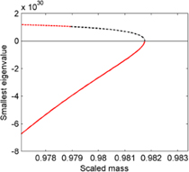
Figure 2. The smallest eigenvalue of the Hessian matrix in capillary model 1 describing two component bubbles at 330 K, for the stable (dashed line), the unstable (solid line) and the metastable region (dash-dot line). The solid line corresponds to small bubbles, and the upper line to large bubbles.
Download figure:
Standard image High-resolution image
Figure 3. The reversible work of formation from capillary model 1 for two-component bubbles at 330 K for the stable (dashed line), the unstable (solid line) and the metastable region (dash-dot line).
Download figure:
Standard image High-resolution image
Another interesting observation is that capillary model 2, when the liquid surrounding the bubble is incompressible, has only one possible bubble solution at a specified total mass of the system, figure 1. This means that assumptions about the compressibility of the liquid will have a large impact on estimates of minimal radii. In the limiting case of an incompressible liquid, there is no minimal radius of the bubble, but when the liquid is compressible, a minimal radius exists. We can address the stability of capillary model 2, through evaluation of ΔW, with homogeneous ideal gas as the reference state. Then the bubbles are always stable. For small drops, the assumption of an incompressible liquid changes the minimal radius of the drop very little.
5. Conclusion
We have investigated how the formation of nanoscale bubbles are limited by a minimal size in systems with constant Ni, V, T (total mass of components, total volume and temperature). We used the square gradient model for curved systems combined with the cubic equation of state, Peng–Robinson, to analyze the system from a mesoscopic point of view, and compared the results to those obtained from the capillary model, which addresses the problem from a macroscopic point of view. For the hexane–cyclohexane mixture, we observed that the capillary model was able to reproduce well the results from the square gradient model in the homogeneous regions, if the value for the surface tension obtained from the square gradient model was used. The minimal radius for a stable bubble in a 38 nm container in this binary system was found to be 8.4 nm, but a thermodynamic stability analysis showed that it was possible to have metastable bubbles down to 6.5 nm. No threshold radius, and only one possible bubble solution corresponding to a stable bubble was found using the capillary model with the liquid assumed to be incompressible. The assumption of incompressible liquid had little effect on the minimal droplet radius. This indicates that a more detailed analysis should be done regarding the role of the compressibility in determining the stability and size of nano bubbles in binary systems.