
Abstract
Laser beam shaping is a venerable topic that enjoyed an explosion in activity in the late 1990s with the advent of diffractive optics for arbitrary control of coherent fields. Today, the topic is experiencing a resurgence, fuelled in part by the emerging power of tailoring light in all its degrees of freedom, so-called structured light, and in part by the versatility of modern day implementation tools. One such example is that of digital micro-mirror devices (DMDs), for fast, cheap and dynamic laser beam shaping. In this tutorial we outline the basic theory related to shaping light with DMDs, give a practical guide on how to get started, and demonstrate the power of the approach with several case studies, from monochromatic to broadband light.
Export citation and abstract BibTeX RIS

Original content from this work may be used under the terms of the Creative Commons Attribution 4.0 license. Any further distribution of this work must maintain attribution to the author(s) and the title of the work, journal citation and DOI.
1. Introduction
Shaping light is purported to have a history dating back thousands of years [1], but gained traction only in the past century with the emergence of micro-electronics. The resulting optical advances in lithography for smaller and faster computing chips had a two fold effect: novel optical elements could now be calculated numerically using computers, while the lithographic fabrication of chips could easily be translated across to optical elements with small feature sizes. The outcome was an explosion in laser beam shaping from around the 1990s with diffractive and computer generated optics [2–5], and even the emergence of the first sub-wavelength structures a decade later for what today might be called metasurfaces [6]. In those early developments, the focus was on tailoring light in amplitude (intensity) using phase as a resource. The polarization of the light was largely considered a complication in wavelength-sized grating that had to be contended with. In recent times this has experienced resurgence in so-called structured light [7, 8], novel optical fields tailored in any degree of freedom, including spatial control of amplitude, phase and polarization. Such shaping can be done internal to the laser, for structured light directly from the source [9], or external to the laser, fuelled by advances in shaping tools [10] such as refractive [11] and free-form optics [12], liquid crystal spatial light modulators (SLMs) [13–15], geometric phase liquid crystals [16–18] and metasurface elements [19], giving rise to exciting advances in novel states of light [20–24].
More recently we have seen the emergence of digital micro-mirror devices (DMDs) as beam shaping tools [25, 26], which have been used extensively for both creation and detection of novel light fields [27–37], gaining in popularity because of their ability to modulate polarization states independently and in real-time [38–40]. Compared to liquid crystal SLMs, DMDs are faster, cheaper, polarization and wavelength insensitive. However, this comes at the expense of optical efficiency [41].
In this tutorial we outline the basic theory and practical steps needed to shape light with a DMD. We use orbital angular momentum (OAM) vortex beams and flat-top beams as two topical case studies, and walk the reader through the required salient steps as well as the pitfalls to avoid. We first outline the general concepts supported by theory before moving on to 'getting started' with practical tips that include alignment, hologram encoding and aberration correction. We then select some case studies and show how to shape monochromatic light, and finally illustrate how to perform broadband beam shaping with a DMD. We believe that this tutorial will be of benefit to readers who wish to enter the field and get up to speed with a DMD in their laboratory.
2. The theory of beam shaping
2It is often not fully appreciated that in-principle lossless and ideal beam shaping can be done with just two phase-only optical elements separated by some distance [42–44]. If instead the shaping is done in a single step then the output is imperfect and/or lossy. One can appreciate this point by considering the simple telescope to resize an optical field: two appropriate lenses (phase-only beam shaping elements) can execute this ideally and in-principle losslessly, while a single lens will correctly resize the beam but at the expense of the phase at the output plane so that the 'shaping' is imperfect. Another example is the creation of OAM vortex beams [45, 46]: single step transformations using an azimuthal phase element results in the correct 'vortex' phase but leaves the amplitude as a free degree of freedom (DoF) where many radial modes are excited with low power content in the desired ring of light [47, 48]. This can be overcome and perfect reshaping achieved in one step, but then the process is lossy, requiring amplitude control, as has been done for the creation of radial mode controlled vortex beams [49]. A similar scenario is seen in another common beam shaping problem, the conversion of a Gaussian beam to a flat-top beam [50–53] subsequently implemented by a variety of means [54–58].
This point is illustrated in figure 1. In figure 1(a) a vortex beam is created in a single step with the correct amplitude and phase, but in a lossy approach using complex amplitude modulation on a single optical element. If a phase-only single element is used, as in figure 1(b), then only one DoF can be controlled. Here it is the amplitude structure of a flat-top beam, with the phase left as a free variable. It requires a second phase-only element to correct this unwanted phase, as shown in figure 1(c). Now the set-up has two phase-only elements separated by some distance, but can in principle execute the desired transformation both ideally and losslessly.
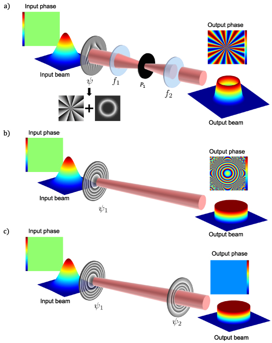
Figure 1. (a) A Gaussian beam is modulated in amplitude and phase in one step by a complex amplitude hologram (ϕ) to create a vortex beam, (b) a single phase only hologram (ϕ1) converts a Gaussian beam to a flat-top beam in amplitude but without phase control, and (c) a second phase-only hologram (ϕ2) can correct the phase to make a two-step ideal and lossless process.
Download figure:
Standard image High-resolution imageSo in general, one-step beam shaping can be ideal but lossy if both amplitude and phase are controlled, while two-step beam shaping can be both ideal and lossless with just two phase-only elements. In the context of this tutorial the term 'lossless' has to be quantified. Neither DMDs nor SLMs are lossless, but this is not an issue of the design but rather its implementation. The term is used in the sense that the design is lossy or lossless, e.g. it could be executed on phase-only elements such as diffractive kinoforms or free-form refractive optics and then could indeed be (in principle) lossless. Encoding the same design on a DMD would naturally incur some loss, but this is by the nature of the choice of implementation only.
Two questions then remain: (1) how does one calculate the desired amplitude and phase profiles, and (2) how does one convert that to be written to a simple binary amplitude device such as a DMD?
2.1. DMD computer generated holograms (CGHs)
We will address the second part first. Imagine that in general you may want to have a CGH that encodes both amplitude and phase, and write this to the DMD. We include amplitude in the desired hologram since for a variety of reasons the reader may wish to execute the beam shaping in an ideal but lossy single step. Say we wish to create the complex amplitude  . How can one write a complex amplitude and phase to a simple binary on/off device to create such a beam? Fortunately this problem was solved nearly half a century ago when sophisticated match filters for pattern recognition were required, but only rudimentary optical elements existed [59]. Both a conventional hologram and a CGH are formed by the interference of a reference plane wave,
  , with an object wave,
  , the conventional hologram done physically and the CGH done computationally. The hologram transmittance is proportional to

where the third term performs the object wave reconstruction. Unfortunately if only a simple binary on/off amplitude-only hologram is possible, then the binary version of the key reconstruction term becomes
which mathematically can be executed by the function
returning 1 or 0 as the sign of the cosine function changes. We see that the amplitude information is lost (no need to insert the  term) since this on/off oscillation is not amplitude dependent, the resulting train of on-off amplitude pulses only holds the desired phase information. To get around this, one introduces a bias function for the clipping level,
  instead of 0, which is equivalent to subtracting it from the original function, namely [59]
so that now the pulse train has leading and trailing edges in its pulses given by solutions to  . The challenge is to find the function q(x). The Fourier series representation of this pulse train can be written as

with
We see that the m = 1 term (T1) has the desired phase,  , and an amplitude factor
 ![$\sin [\pi\! q(x)]/ \pi$](https://content.cld.iop.org/journals/2040-8986/25/7/074003/revision4/joptacd563ieqn8.gif) . Since we will normalise all amplitude to 1 anyway, if we simply set
. Since we will normalise all amplitude to 1 anyway, if we simply set ![$A(x) = \sin [\pi\! q(x)]$](https://content.cld.iop.org/journals/2040-8986/25/7/074003/revision4/joptacd563ieqn9.gif) so that
so that ![$\pi q(x) = \arcsin [ A(x) ]$](https://content.cld.iop.org/journals/2040-8986/25/7/074003/revision4/joptacd563ieqn10.gif) then we have our solution. The DMD hologram then becomes
then we have our solution. The DMD hologram then becomes
where now we have written it in two-dimensions (for a 2D pulse train). It is worth unpacking this function. The encoding can be understood as larger pulse widths in the pulse train leading to larger amplitudes being diffracted into the first order, while local shifts in the pulse position allow for propagation phase control through small path length differences. Note that the input to the pulse train is the desired amplitude and phase of the output beam, which is now formed in the near-field, at the plane of the DMD. The desired beam is separated from the undesired diffraction orders by virtue of the blazed grating (our reference wave), of the form  with periods λx
and λy
in the x and y directions, respectively. This alters the diffraction angle of the desired light relative to the zeroth-order by
with periods λx
and λy
in the x and y directions, respectively. This alters the diffraction angle of the desired light relative to the zeroth-order by  and
and  , and is referred to as an off-axis design. Because this requires propagation, it is common to use a telescope to map angles to position in the Fourier plane, separate out the desired beam, and then return to the plane of the DMD but now with only the desired field (see examples later). The
  function binarizes the output so that the function returns 1 for
  or 0 (all else), ensuring the binary on/off input to the DMD as per equation (4). The low efficiency can be appreciated by noticing that only the T1 component has the desired amplitude and phase, with the other terms T2, T3 and so on all carrying unwanted light.
One can further explore this function by reframing the problem in terms of the pulse train itself. The one dimensional (1D) binary amplitude grating is a pulse train of the form
where m represents each opening in the grating at the position p of width w, with period λx . Now we wish to relate these pulse train parameters to the amplitude and phase of the hologram. We can expand T(x) into a Fourier series to find [25, 60]
and
We can see that the coefficients Tm
dictate the amplitude and phase diffracted into the mth order. If this binary amplitude grating represents the on/off states of the light, then for instance, T1 is an amplitude and phase associated with the plane wave at angular frequency  , T2 is an amplitude and phase associated with the plane wave angular frequency
  , and so on. Using T1 as an example, we see now that we can find solutions for the unknown p and w from
from which we immediately find that we need to make the pulse width w and position p spatially varying according to
relating the train parameters to the desired beam parameters. We see that indeed the amplitude is now encoded into the width of each pulse, with the period holding the phase information. The solution is identical in 2D by replacing  in the arguments of all functions in the solutions, i.e.
so that now we have a two-dimensional pulse train. In the rest of the tutorial we will use specific examples of desired amplitudes and phases in order to make the treatment practical, and to do so we select from common beam types.
2.2. Beam types
In this tutorial we will refer to three common beam types [61]. The first is the familiar Laguerre–Gaussian (LG) modes, a subset of circularly symmetric solutions of the paraxial wave equation, written in cylindrical coordinates (r, φ, z) as
where p and  are the radial and azimuthal indices respectively, and
  is the generalised Laguerre polynomial. The functional arguments take the form of
and

where w0 is the Gaussian (fundamental mode) radius at its waist plane (z = 0) and λ is the wavelength of the light. Such modes are shape (but not size) invariant during propagation. The OAM modes are identified by the azimuthal phase term  , where the topological charge,
  defines the helicity of the phase, for
  phase twists about the azimuth and
  of OAM per photon. The twist can be clockwise or anticlockwise for an alphabet that spans
 ![$\ell \in [-\infty,\infty]$](https://content.cld.iop.org/journals/2040-8986/25/7/074003/revision4/joptacd563ieqn25.gif) , and hence the term vortex beams or twisted light to describe OAM light.
, and hence the term vortex beams or twisted light to describe OAM light.
These complex modes reduce to the special case of the Gaussian beam when  . In this case
Finally, a flat-top beam can be approximated by a Super-Gaussian function of the form
where Γ is the Gamma function and w is a radial size parameter. Such beams are not propagation invariant and do not have a simple analytical expression that includes z. The Super-Gaussian order, N, determines both the flatness of the peak and the steepness of the edges, reducing to a Gaussian beam when N = 2 and becoming an ideal flat-top beam at large N. Unless stated otherwise, we will always assume in the tutorial that the desired beam is that as defined at z = 0. Note that all the aforementioned functions describe the optical field in amplitude and phase.
2.3. Calculating the transmittance function
How should we calculate the desired transmittance function of the DMD holograms? There are two options available. In Method 1, we apply complex amplitude modulation, that is, we alter both the amplitude and phase of the incoming beam to tailor it to the desired output, which can be done in a single step with loss. If the incoming beam is  and the output beam is
  then the transmittance function is
with the requirement that the amplitude is normalised such that light is only removed and not created. In many instances it is convenient to overfill the DMD to mimic a plane wave so that  and the hologram is identical to the amplitude and phase of the desired output beam. There are several recipes to make this suitable for DMDs [59, 62].
In Method 2, two elements are used, both in principle phase-only, so that the execution can be lossless, although not on a DMD. The first element redistributes the energy to shape the desired amplitude, leaving the phase as a free variable, and the second element corrects for the phase. The two elements are separated by some distance to allow the energy redistribution, which is usually a focal distance from a lens incorporated into the first element (the far-field being the farthest that one could propagate).
To derive the phase of the first element,  we need to find a mapping function from the input beam to the output beam that moves energy from a specific spatial region of the input beam to a specific spatial region of the output beam while conserving energy. It is the calculation of this mapping function, α, which lies at the heart of the method. This has been outlined for the arbitrary creation of structured light [63, 64], and here we summarise the key steps as part of the tutorial. If the input beam is passed through an element with phase
  and a lens, and both the input and output beam are energy normalised to 1, then at the focal plane of the lens we have
Recall that  since it maps co-ordinates (and energy) from the input to the output plane, so that
By setting  and
and  we have that
Equation (22) can be evaluated by the method of stationary phase as
with
If we have devised  correctly then we have that
  and so
This can be reduced to solving for  (in one-dimensional Cartesian coordinates) as
This equation describes how energy can be mapped from the input profile to the output profile in a manner consistent with the conservation of energy. The phase  can then be easily calculated from the expression for α. The phase is
Once the first phase element has been designed there are two viable approaches to designing the second phase element: in some approximations (short focal lengths and smooth beams) the second phase element can be well approximated as the complex conjugate of the first shaping element, otherwise the phase of the output beam from the system can be calculated and the second element given an appropriate correction. For example, if the input field is now mapped to an output of  rather than
  , then the second phase correcting element requires a phase of
  .
.
To illustrate the role of phase-only versus amplitude and phase encoding, consider the examples shown in figure 2 for the scenarios of (a) creating a vortex beam by a phase-only function on an SLM (with desired transmittance  ), (b) a complex amplitude function on an SLM (with desired transmittance
  ), and (c) a complex amplitude function on a DMD (with desired transmittance
  ), respectively. The panels show the hologram form and a cross-section along the dashed red line on the right. The smooth phase-only function in (a) is in contrast to the modulated version to contain amplitude information in (b), and finally the binary amplitude version in (c). The simulated outcome of the nearby diffraction orders is also shown. In all cases the desired beam is in the +1 order. The pulse train in (c) now visualises the role of the functions p and w.
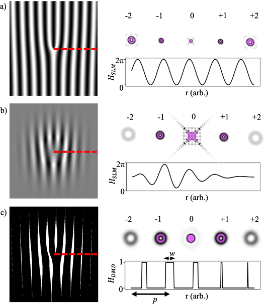
Figure 2. Computer generated holograms for creating a vortex beam by (a) a phase-only function on an SLM, (b) a complex amplitude function on an SLM, and (c) a complex amplitude function on a DMD. The main frames show the hologram with the insets depicting the simulated output for various diffraction orders. A cross-section of the hologram is shown along the dashed red line as an inset.
Download figure:
Standard image High-resolution imageWhat remains is to consider the effects of broadband shaping. Imagine that the desired transmittance function is  and that added to this is a blazed grating of the form
  . One can show that the effect of designing the phase element for wavelength λ0 but actually operating at wavelength λ is to alter the action of the transmission function to [65]
We see that in the first diffraction order, m = 1, we have the desired field but modulated in amplitude by a constant factor ![$\eta = \mathrm{sinc} [{\pi}(1 - \lambda_0 / \lambda ) ]$](https://content.cld.iop.org/journals/2040-8986/25/7/074003/revision4/joptacd563ieqn47.gif) . When
. When  we find that η = 1, as expected, decreasing as the difference in wavelength increases. What this means is that the operation of the element will remain intact and wavelength independent except for a small decrease in efficiency as the design wavelength is altered (less than 1% in the experiments reported in this tutorial). There is however one downside. The angle at which light is diffracted is still wavelength dependent, following the familiar rule for periodic structures of
  , where θm
is the angle of the mth order. A consequence is that the desired light will be created for all wavelengths, but they will appear to emerge at different angles, thus at different positions in the far-field. This dispersion effect has to be corrected in the experiment by using a compensating element such as a grating or prism [66].
, where θm
is the angle of the mth order. A consequence is that the desired light will be created for all wavelengths, but they will appear to emerge at different angles, thus at different positions in the far-field. This dispersion effect has to be corrected in the experiment by using a compensating element such as a grating or prism [66].
3. Getting started with DMDs
In this section we introduce DMDs. Beginning with a description of their structure and operating principles, we then provide a summary outlining experimental techniques that have proven to produce the highest efficiency and beam quality, thus setting the foundation for optimal beam shaping with DMDs.
3.1. DMD structure and operation
At present all commercially available DMDs consist of two main components: a micro-mirror array (the screen) and a set of electronics (the driver unit) that controls the mirrors, as depicted in figure 3.
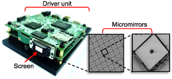
Figure 3. The DMD consists of two main components: the driver unit and screen (as labelled). The screen consists of a micro-mirror array comprised of individual micro-mirrors (inserts).
Download figure:
Standard image High-resolution imageAlthough there are a variety of commercially available DMDs of different sizes and resolutions, DMDs are generally classified by the layout of their micro-mirror array. There are two distinct layouts of the micro-mirror array: Cartesian and diamond, as seen in the figures 4(a) and (b) respectively. In a Cartesian layout the micro-mirrors (depicted as white squares) are arranged in a manner resembling a Cartesian grid, i.e. the mirrors' axes (depicted by green dashed lines with xʹ, yʹ) are aligned parallel to the axes of the base (depicted by blue solid lines with x, y) the mirrors are attached to. In this layout, the micro-mirrors have a separation distance d between adjacent micro-mirrors' centres (depicted by red arrows) that is equivalent in both the vertical and horizontal directions. In a diamond layout, however, the micro-mirrors are rotated at a 45∘-angle relative to the base, making the square mirrors appear diamond-like. To optimize the packing of the micro-mirrors in a diamond layout, the mirrors are arranged so the separation distance in the horizontal direction, 2d, is twice the distance in the vertical direction, d. The difference between the two layouts must be taken into account when encoding holograms onto different DMD models.

Figure 4. Based on the model, DMDs have different layouts of their micro-mirror arrays. In (a) a Cartesian layout the micro-mirrors (depicted as white blocks) are arranged in a manner resembling a Cartesian grid where the micro-mirrors axes (depicted as dashed green arrows with xʹ, yʹ) are aligned to axes of the base (depicted as solid blue arrows with  ) that they are attached to. The separation distance between the micro-mirrors' centres in the x direction, d is equivalent to the separation distance in the y direction. In a (b) diamond layout the micro-mirrors are rotated at a 45∘ angle relative to base. In this layout the square micro-mirrors appear 'diamond like'. To maximise the packing efficiency, the separation distance between the mirrors' centres in the vertical direction, 2d is twice the separation distance in the horizontal direction, d.
Download figure:
Standard image High-resolution imageFor example, the DLP 3000 series (Texas Instruments) has a resolution of  pixels orientated in a diamond layout; its square micro-mirrors have a width and height of 7.6 µm, a separation distance d = 10.8 µm between adjacent micro-mirrors, and an array fill factor of 92% [67]. On the other hand, the DLP 6500 series (Texas Instruments) has a resolution of
  pixels orientated in a Cartesian layout; its square micro-mirrors also have a width and height of 7.6 µm, a separation distance d = 10.8 µm between adjacent micro-mirrors, and an array fill factor of 92% [68]. Since the pixel sizes and array fill factors are the same for both models, the difference in efficiency can be considered negligible. In other words, despite the micro-mirror array layout the DMD will have a maximum efficiency of ≈6% in the +1st order, where one would observe the desired structured mode [25]. Hence when selecting a DMD, the only parameters to consider are the DMD's resolution and its overall size. For example, the DLP 6500 has a higher resolution which could result in a higher purity mode. However, the trade-off is the DMD's relatively large size (≈400 mm × 120 mm × 50 mm) which may pose a problem in certain spatially-restricted applications. In comparison, the DLP 3000 may have a lower resolution, which could result in a lower purity mode, but it is relatively compact (≈80 mm × 70 mm × 30 mm). In this tutorial we have chosen to use a DLP 3000.
Micro-mirrors are small, highly-reflective aluminium squares that pivot about their diagonal and reflect the incident light. The movement of the micro-mirrors are made possible by the torsion hinges they are attached to. However, the spring tips restrict the micro-mirrors' possible rotation angles, causing the incident light to be directed at  off axis. By convention the positive (+) state is referred to as ON and the negative (−) state is referred to as OFF. Micro-mirrors in the ON state direct light toward the desired direction and micro-mirrors in the OFF state direct light in the opposite direction. When powered and operational all micro-mirrors in the DMD must occupy one of the two states. However, when the DMD is non-operational all mirrors are in a 'parked' state where they are neither ON nor OFF. In this state the mirrors are not controlled by the driver, so they are not held at a fixed angle. Therefore, when in the 'parked' state the micro-mirrors are roughly parallel to the base that the mirrors are attached to. Figure 5 shows the possible orientations of the micro-mirrors.
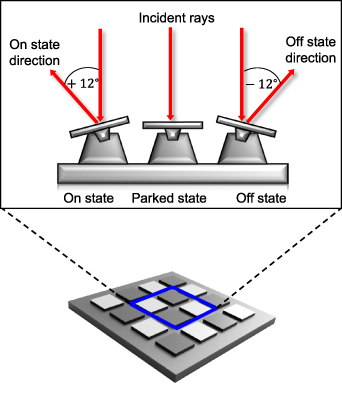
Figure 5. The three possible states of the DMD micro-mirrors: ON, parked and OFF. When non-operational the micro-mirrors are in the 'parked' state. When operational the micro-mirrors will either be ON or OFF and deflect the incident light at a angle  relative to normal incidence.
Download figure:
Standard image High-resolution imageNote that a consequence of the DMD mirror angles in the ON and OFF states is that the zeroth order is necessarily redirected at this angle too. This should be seen as the new beam direction of the outgoing light. The modulated light can be sent at this angle too by simply forgoing the grating, or the grating can be use to cancel out this redirection, as has been done in the creation of on-axis vectorial beams [40]. In other words, the final direction of the modulated light can be tailored more or less at will by the incoming angle of incidence and the grating period.
By reflecting light in the desired direction, or deflecting it away, the DMD is able to manipulate the incident beam's amplitude, and as we have discussed in the theory of section 2, this can be leveraged on for other degrees of freedom too. However, to do this one must have complete control over each micro-mirror in the screen by addressing it with a 0 or 1 for an OFF or ON state as a pixelated hologram.
3.2. Pixel considerations
Implementing CGHs on a pixelated device entails the computation of a two dimensional matrix with dimensions that match the resolution of the device's screen. Each element in the matrix has a one-to-one mapping to a micro-mirror on the device, hence it is important to encode the correct dimensions too. Since each micro-mirror can occupy one of two states when operational (the ON or OFF states), the DMD is considered to be binary in nature, hence the matrix must be binary too, with each element having a value of 0 or 1. When this matrix is encoded on the DMD, the driver interprets a value of 0 as an instruction for that particular micro-mirror to occupy the OFF state, and a value of 1 for the micro-mirror to occupy the ON state.
To visualise the matrix, we assign colours to each value and thus create a binary hologram. Because light is directed towards the desired plane when the micro-mirrors are in the ON state, the matrix element or pixel is assigned the colour white in the hologram. However, because light is directed away from the desired plane when the micro-mirrors are in the OFF state the pixel is assigned the colour black. Figure 6 illustrates the relationship between the generated binary matrix, the hologram and the micro-mirrors' states.
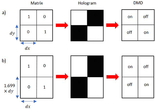
Figure 6. Holograms act as a means to control each micro-mirror in the DMD's screen. First a binary matrix with the same dimensions as the DMD's screen is generated. (a) For DMDs with a Cartesian micro-mirror array layout, each matrix element has a vertical size equivalent to the micro-mirror's height  and a horizontal size equivalent to the micro-mirror's width,
  . (b) For a DMD with a diamond micro-mirror array layout, the orientation of the mirrors must be taken into account as mentioned by [25]. Hence each matrix element is up-scaled by a factor of 1.699 in the vertical direction relative to the micro-mirror's height
  , i.e. each element will have a vertical size of 1.699(
 ). However, each matrix element will have a horizontal size equivalent to the width of the micro-mirror,
  . To visualise this matrix, each value is assigned a colour i.e. the colour black is assigned to elements with a value of 0 and white is assigned to the elements which have a value of 1. In this way a binary hologram is created, which can be encoded on the DMD. Because each element in the hologram has a one-to-one mapping with each micro-mirror in the DMD's screen, in essence the colour of the hologram element or pixel corresponds to the micro-mirror's state. Hence, when the element is coloured black it corresponds to the micro-mirror in the 'off' state, and when it is coloured white it corresponds to the micro-mirror in the 'on' state. In this way one can control the micro-mirrors in DMD.
Download figure:
Standard image High-resolution imageThe layout of the micro-mirror array must be taken into account when designing the geometry of the pixel array, otherwise an elliptical distortion of the beam may be observed. It was shown that for DMDs with a diamond layout, one simply needs to upscale the initial matrix's dimensions in the vertical direction to compensate for this incorrect mapping. This scaling factor was determined in an iterative manner until it converged to the ideal ratio of the vertical and horizontal pixel size of 1.6889. In other words when encoding the hologram matrix, the vertical dimension (or y coordinates) should be upscaled by a factor of 1.6889. When this is done, the hologram matrix will be correctly mapped and the beam will no longer appear elongated. Figure 6(a) shows an appropriate mapping for a Cartesian micro-mirror array, with figure 6(b) showing an example for the diamond geometry, where the pixel size in the vertical direction is up-scaled by a factor of 1.699. The outcome experimentally of using the incorrect or correct scaling is shown in figure 7: in (a) we see an elongated beam when no scaling is applied but the hologram is displayed on a diamond geometry device, with part (b) showing the same hologram correctly scaled.
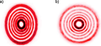
Figure 7. (a) Incorrect scaling of the hologram resulting in an elongated beam, and (b) correct scaling of the hologram resulting in a symmetric beam.
Download figure:
Standard image High-resolution image3.3. Optical considerations
Before using a DMD to conduct experiments it is important to ensure that it is correctly set up and aligned. It is also imperative to know the optimal properties and parameters related to the DMD. In this subsection we outline the necessary experimental techniques and optical setups needed to achieve maximum efficiency and beam quality.
3.3.1. The incoming beam.
A common working configuration for a DMD, shown in figure 8, is to use an expanded and collimated beam as the incident field. This ensures that the beam has a flat wavefront with a uniform intensity distribution, comfortably fills the DMD screen, and may be apertured for size as needed. It is important to note that collimation is only necessary when doing amplitude-only and complex-amplitude modulation as it involves the 'carving' out of the incident light to form the desired shape. This is easily achieved with a suitable telescope prior to the DMD. Telescope solutions have the benefit of preserving amplitude and phase structure as they simply relay the object plane to the image plane, but with a nett magnification given by the ratio of the focal lengths. Single lens imaging systems do not preserve phase information and should be used with caution.

Figure 8. A schematic illustrating a typical experimental arrangement for aligning the DMD. After expansion and collimation of the incoming laser light with the aid of two lenses [l1 (f1) and l2 (f2)], the expanded light is apertured (P1) to control the beam size incident on the DMD. When the DMD is encoded with a grating, the output beam is be separated into diffraction orders ( are shown). The inset depicts the two possible alignments of the DMD, either (a) tilted at an angle of 12∘ or (b) normal to the incoming light.
Download figure:
Standard image High-resolution imageTo ensure the maximum efficiency and beam quality the DMD should be centred and tilted at 12∘ relative to the incident beam, as shown in figure 8(a). To do this a hologram should be encoded on the DMD that sets all the mirrors to the OFF state so that the back reflected light can be aligned to the incident beam. An alternative, less efficient method is to aligned the DMD at 0∘ as illustrated in figure 8(b), with the device not powered and the mirrors in a parked state. Through back reflection the beam is then aligned to the incident beam. In this configuration, mirrors in the ON and OFF states will reflect the output beam at  relative to the normal incident beam.
3.3.2. Sorting diffraction orders.
The grating encoded in binary holograms leads to the incident beam being separated into diffraction orders, where the +1st order (m = 1) mode has the correct phase and structure. To calculate the spatial position or angle of any of these orders, consider the diffraction grating equation

where m is the diffraction order number, θm
is the diffraction angle for order m, λ is the incident wavelength and λx
is the grating period (here shown for the x direction). This is illustrated in figure 9, where a binary grating applied to the DMD, creates both  orders as well as the unconverted m = 0 order, shown for a Gaussian input. The angles for each order determine the location of the spots in the Fourier plane, one focal length after a lens, and are given by
  . Similarly, for the y off-set if there is a grating in y with a period λy
. The physical separation of the beams allows one to select the desired order by a simple aperture. A second lens to form the image plane of the DMD recombines the light back to a single spot.
. Similarly, for the y off-set if there is a grating in y with a period λy
. The physical separation of the beams allows one to select the desired order by a simple aperture. A second lens to form the image plane of the DMD recombines the light back to a single spot.
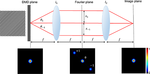
Figure 9. A Gaussian beam is incident on a binary grating displayed on a DMD, producing new diffraction orders of  . A Fourier transforming lens maps angles (
 ) to positions (
 ) in the Fourier plane, while a second lens reverses the process to return to the image plane of the DMD screen.
Download figure:
Standard image High-resolution imageTo ensure that there is no overlap between the orders, appropriate grating periods of λx and λy in the x and y directions, respectively, should be chosen. If the grating period is too low the orders will not be well separated, and if the grating frequency is too high ghost orders (a replica of the higher order modes) will appear. In both cases this will lead to an increase in background noise and/or a distortion of the mode.
Before aligning the output from the DMD, one needs to locate the +1st order diffracted beam. Against popular belief, the DMD does not act as a blazed grating [25]. Hence the +1st order beam is not necessarily the brightest one, making it difficult to distinguish from the other orders. This can be solved by programming a converging lens and a grating onto the DMD. To see how this works, consider the flow diagram shown in figure 10. An incoming Gaussian beam is imparted with a lens and grating phase, resulting in it forming a converging beam in the +1st diffraction order and a diverging beam in the −1st diffraction order (the 0th order is not influenced by the hologram phase). As shown in the right-hand panel, the +1st beam will be smallest near the focal plane of the programmed lens, and is therefore easy to locate. So long as the grating period is not changed, the desired order will remain in the same position and can be selected with a judiciously sized and placed aperture.

Figure 10. When a Gaussian beam is incident on a DMD encoded with a grating and converging lens, the output beam will diffract into orders that are converging, diverging or unaltered, shown here for  . The desired +1st order will be the smallest in size compared to the other orders at a distance close to the programmed focal length, making it easy to identify and thus single out with an aperture.
Download figure:
Standard image High-resolution image3.3.3. Aberration correction.
Aberrations are an inherent property of any optical element or system that arises from imperfections introduced during the manufacturing process and/or through wear-and-tear. Imperfections are not always noticeable and easy to locate, yet they can severely distort a structured beam. An example of this is shown in figure 11(a) for a DMD that is both misaligned and aberrated. Correcting the alignment by following the steps already outlined results in a marginal improvement as shown in figure 11(b), but the vortex splitting into many vortices is now clearly evident by the five central intensity nulls along a diagonal line. Correcting for the device aberrations produces the desired beam in figure 11(c). This example illustrates why aberration correction is a vital step when using DMDs. A good way to describe the aberrations is to use the Zernike polynomials with weighting coefficients to describe the wavefront as

Figure 11. Experimental images depicting the effect misalignment and aberrations have on a structured vortex (l = 5) beam. (a) Misaligned and aberrated, (b) aligned and aberrated, (c) aligned and corrected for aberrations.
Download figure:
Standard image High-resolution imagewhere Cj
are the Zernike coefficients (units of waves) for the corresponding  Zernike polynomial
  . A wavefront sensor can do this decomposition, but it is often more convenient to use the structured light itself as a probe. To this end, vortex modes with a low OAM value
  are extremely sensitive to any phase distortions. When observed in the Fourier plane these irregularities are converted to amplitude distortions, making it easier to identify: take another look at the vortex splitting in figure 11(b). By adjusting the correcting phase until the beam is pristine, the aberrations in the entire path to the detector are corrected, including that of the DMD.
When doing aberration corrections a semi-empirical approach is the easiest to implement. Often, first-order astigmatism is the main contributor of aberrations to the system. Therefore, by encoding Zernike phase maps corresponding to first-order astigmatism, or any other prominent aberration, and manually adjusting the weighting coefficients of these polynomials until the vortex mode appears 'perfect' in the Fourier plane, one can correct for much of the phase error. The weighting coefficients represent the root-mean-square wavefront error attributed to the respective aberration and they are independent of the number of polynomials used in sequence [69]. In other words, coefficients of a term can be changed without it affecting other polynomial terms.
It is important to note that in some cases, DMDs have a prominent defocusing aberration associated with it. Unlike astigmatism or other aberrations, the defocusing aberration cannot be corrected for in a traditional manner. To correct for the defocusing of the DMD a converging lens must be encoded with a focal length that is exactly equal to the separation distance of the DMD and observation plane. The weighting coefficient of the defocus Zernike polynomial should then be adjusted until the mode is the smallest size.
Finally, to optimise the setup one must do a fine alignment to account for minute misalignments. This cannot be easily seen if the beam is quite distorted, hence aberration correction is usually done first. To do this the DMD is now encoded with a hologram consisting of a grating (the same frequencies as before) and a mode with a circular shape, for example a vortex l = 5 (in this case a high OAM value is preferable). The modulated +1st order beam should be singled out using an aperture. If the DMD is misaligned as seen in figure 11(a), then as the aperture in the expansion and collimation system is closed so the intensity of the beam will be reduced. To correct for this misalignment the encoded hologram needs to be shifted in the x–y plane until the beam appears perfect, as seen in figure 11(c). This can be done by shifting the x–y coordinates when creating the matrix for the hologram code. If the shift required is large, the DMD itself should be shifted slightly using the translation stages it is mounted on.
4. Monochromatic beam shaping
As mentioned in section 2 one can shape light in a lossless manner through phase-only or both phase and amplitude (complex-amplitude) modulation. In this section we explore how to use a DMD to shape monochromatic light using both methods. To do this we select two examples: (1) the creation of a flat-top beam from a Gaussian using a phase-only solution, and (2) the creation of a LG beam by complex amplitude modulation from an input plane wave.
4.1. Creating flat-top beams
In the first example, a Gaussian beam is incident on an element with desired the phase-only transmittance ![$t(r) = 1 \exp[i \varphi(r)]$](https://content.cld.iop.org/journals/2040-8986/25/7/074003/revision4/joptacd563ieqn71.gif) followed by a lens with transmittance
followed by a lens with transmittance ![$t_\text{lens} = \exp [-i k r^2/(2 f\,)]$](https://content.cld.iop.org/journals/2040-8986/25/7/074003/revision4/joptacd563ieqn72.gif) , where f is the focal length of the lens. The desired flat-top beam is located at a distance f after the lens. To understand the role of the lens, consider the following: when performing phase-only modulation the beam shaping element, a DMD in this case, imparts a phase change to the incident coherent light that causes a redistribution of the Gaussian's intensity until it is uniform, i.e. a flat-top. Although this phase change occurs at the DMD's plane, it is noticeable as an amplitude effect as the beam propagates. Hence, when performing phase-only modulation the beam should be observed in the far field where it will have the desired phase and structure of a flat-top. This process is illustrated in figure 12. Using the theory in section 2, one can solve this problem in integral form to find
, where f is the focal length of the lens. The desired flat-top beam is located at a distance f after the lens. To understand the role of the lens, consider the following: when performing phase-only modulation the beam shaping element, a DMD in this case, imparts a phase change to the incident coherent light that causes a redistribution of the Gaussian's intensity until it is uniform, i.e. a flat-top. Although this phase change occurs at the DMD's plane, it is noticeable as an amplitude effect as the beam propagates. Hence, when performing phase-only modulation the beam should be observed in the far field where it will have the desired phase and structure of a flat-top. This process is illustrated in figure 12. Using the theory in section 2, one can solve this problem in integral form to find
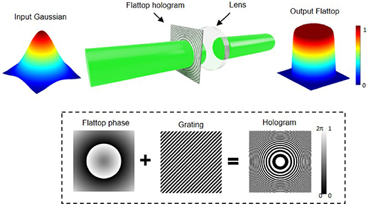
Figure 12. A Gaussian beam is modulated in phase and passed through a lens, with the desired output flat-top beam observed in the focal plane of the lens. The flat-top hologram consists of a flat-top phase (following the theory) and a grating, which are then binarised for display on the DMD. Aberration correction is not shown (but always applied) for pedagogical reasons.
Download figure:
Standard image High-resolution image
where
Here w0 is the  Gaussian radius and w is the flat-top beam size. When β is large (
 ) the solution is easy to implement, the flat-top will be of a high quality, and the geometric approximations are valid. In this one-step solution, the first shaping element converts the Gaussian into a flat-top beam while leaving the phase as a free parameter, implying that we would need a second shaping element, such as a lens, to correct the phase. We have not manually added a grating since this is already assumed in equation (7). Thus the desired hologram to be encoded on the DMD has the following form and can be visualised in the inset of figure 12:
A simulation of the outcome is seen in figure 13, where an incident Gaussian beam (left) is converted into an output flat-top beam (right).

Figure 13. The simulated results of converting an incident Gaussian (left) through phase-only modulation to an output flat-top beam (right) using a hologram that would be encoded on a DMD. The cross sections of the individual modes are shown with their respective intensity profiles depicted as insets.
Download figure:
Standard image High-resolution imageTo demonstrate this process experimentally, we use the system as seen in figure 14(a). In this experiment a monochromatic beam (λ = 514 nm) was imaged onto the DMD using lenses l1 (f = 100 mm), l2 (f = 100 mm). Imaging the beam allows us to control the incident beam size, an important factor when generating flat-top beams. The DMD was encoded with a hologram depicted in figure 14(b), consisting of the desired phase, a grating and aberration correction, before binarisation for the DMD. A lens and aperture were used to select the desired diffraction order, with the lens acting as a Fourier transforming element (as needed in this design approach). It would be ideal to place the aperture in the Fourier plane as the beams are smallest in size, making it possible to discard most of the 'noise' from unwanted orders, however because the scalar flat-top beam is only formed in the Fourier plane the charge-couple device (CCD) camera must occupy this position to allow us to observe the desired flat-top. Figure 14(c) depicts the experimental output flat-top beam's intensity profile and corresponding cross section. The experimental flat-top has a correlation value of 94.9% to simulation, indicating that DMDs can indeed be used to create a structured light through phase-only modulation.

Figure 14. The experimental process of making a flat-top beam. (a) The experimental setup: a monochromatic beam (λ = 514 nm) was imaged onto the DMD using lenses l1 (f = 100 mm), l2 (f = 100 mm). The DMD was encoded with (b) a hologram comprising of a flat-top phase mask, grating and aberration correction phase mask. The incident beam was then modulated and diffracted into its various orders. A lens, l3 (f = 200 mm) was placed a focal length away from the DMD and Fourier transforms the modes. Slightly before the Fourier plane, an aperture P1 was inserted to single out the +1st order. A CCD camera was placed in the Fourier plane, allowing us to observe the desired flat-top. (c) The experimental incident Gaussian and output flat-top beams are shown with their respective cross sections.
Download figure:
Standard image High-resolution image4.2. Creating vortex beams
In the second example, we want to create vortex beams in the manner illustrated in figure 15. In this case the incoming beam is expanded to be a near plane wave, that is, constant phase (collimated) and amplitude normalised to  . The desired beam is to be created by modulating both the amplitude and phase in proportion to a vortex beam of
  , therefore the transmittance function is
  , normalised so that the peak value is 1, to match the incoming amplitude. The amplitude modulation carves out the desired function from the incoming field, similar to a cookie cutter, while the phase term imparts the azimuthal variation. Noting that the azimuthal angle is
  , the desired hologram for the DMD for this second case is
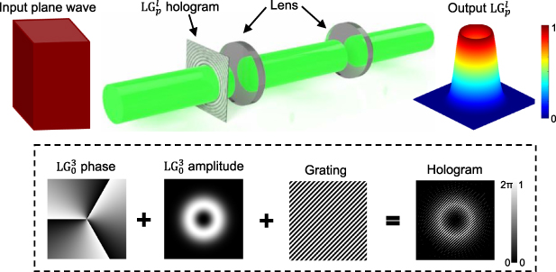
Figure 15. The process of making an LG beam: an expanded and collimated beam (plane wave) is incident on a beam shaping element which structures the incident light through complex-amplitude modulation. The beam then passes through a telescope that translates the generated mode to the image plane. In an ideal case, such as a simulation the LG mode can be generated by (inset) a hologram that comprises of the desired amplitude, phase and lens masks as well as a grating. Using this hologram we are able to structure the incident beam through complex-amplitude modulation. (c) The simulated intensity profiles and cross sections of the incident Gaussian and output LG
 beams are given.
Download figure:
Standard image High-resolution image
and can be visualised as depicted in the inset of figure 15. By using this hologram we are able to manipulate both the phase and amplitude of the incident beam and generate the desired  mode. In this case the vortex beam is created at the plane of the DMD. One could simply allow it to propagate away, slowly separating from the other diffraction orders, but this will introduce additional phases via the z dependent terms in the LG function. Instead, one can image the DMD plane with a telescope, relaying the desired mode away from the DMD to a more manageable optical plane. By encoding the telescope digitally we are able to simulate the process of manipulating the input Gaussian beam (left panel of figure 16) through complex-amplitude modulation into the desired LG mode (right panel of figure 16).
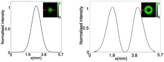
Figure 16. The simulated results of converting an incident Gaussian (left) through complex-amplitude modulation to an output LG beam (right) using a hologram that would be encoded on a DMD. The cross-sections of the individual modes are shown with their respective intensity profiles depicted as insets.
Download figure:
Standard image High-resolution imageTo demonstrate this experimentally we setup the system as depicted in figure 17(a). In this experiment a coherent beam (λ = 514 nm) was expanded and collimated (refer to section 3) by l1 (f = 100 mm) and l2 (f = 300 mm). Aperture, P1 controls the size of the incident beam, as discussed in section 3. The DMD was encoded with the above mentioned hologram, however an additional phase mask was added to correct for inherent aberrations in the system, as seen in the figure 17(b). When the collimated beam was incident on the DMD, it was then diffracted and modulated. The diffracted beams then passed through l3 (f = 200 mm) where the +1st order was singled out by aperture P2, located in the Fourier plane of l3. The +1st order then passed through l4 (f = 200 mm) which images the beam. Using a CCD camera, the  beam was observed in the image plane of the DMD. Figure 17(c) shows the experimentally produced
  mode which has a correlation value of 98.6% when compared to simulation, thus indicating that DMDs can be used for monochromatic complex-amplitude modulation.

Figure 17. (a) The experimental setup: a monochromatic beam (λ = 514 nm) is expanded and collimated using lenses l1 (f = 100 mm), l2 (f = 300 mm) with aperture P1 controlling the beam size. The beam is then incident on the DMD that has been encoded with (b) a hologram comprising the LG phase and amplitude, a grating and aberration correction. A telescope made of lens l3 (f = 200 mm) and l4 (f = 200 mm) images the DMD plane to that of the CCD camera, with an aperture P2 is inserted to single out the desired diffraction order. (c) The experimental output beam is shown with its intensity cross-section.
Download figure:
Standard image High-resolution image5. Broadband beam shaping
In this section we build upon section 4 and extend the same tools and techniques to shape multiple wavelengths of light with a DMD. To do this we must remove or compensate for any wavelength-dependency in the theory, optics and system as a whole. We have already shown theoretically that a simple grating will remove any wavelength dependency of the hologram, at the expense of a small efficiency drop and dispersion of the grating itself. In this section we first demonstrate that indeed the shaping can be wavelength independent, and then address the issue of dispersion compensation of the grating.
5.1. Wavelength independent beam shaping
We first simulate the beam shaping problem, with an example of LG modes shown in figure 18. We used a design wavelength of λ0 = 488 nm and two additional off-design wavelengths of λ = 457 nm and  514 nm. The results shown in figure 18(a) shows that all three modes have identical amplitude and phase structure. For enhanced visualisation, we then converted each image into its true colour using the 'spectrumRGB' function (available on MatLab's open source [70]) which takes an input wavelength value and outputs an RGB value that corresponds to the wavelength's true colour, as seen in figure 18(b). The individual beams' images were then imported as matrices in MatLab, added together and normalised. The result was a digital broadband beam with the correct amplitude and phase structure, depicted in its true colour, as seen in figure 18(c).
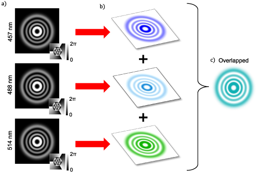
Figure 18. (a) Simulated multi-wavelength LG modes, all created with a hologram designed for
  nm. The intensity is shown in grayscale with the phase shown in the insets. (b) True colour visualisation of each mode using the 'spectrumRBG' function on MatLab. (c) The individually coloured simulation matrices are then added together and normalised for an overlapped multi-wavelength beam.
Download figure:
Standard image High-resolution imageTo verify this process we used the setup seen in figure 19(a), where the desired mode was a broadband flat-top. The experiment was conducted as follows: a broadband beam comprised of three wavelengths (λ = 457 nm, 488 nm, 514 nm) was emitted from an Argon-ion laser. Using two achromatic lenses, l1 (f = 100 mm), l2 (f = 100 mm) this beam was imaged onto the DMD which was encoded with the same experimental flat-top hologram as seen in the inset of figure 19(a), where  488 nm. All alignment and aberration correction procedures were performed using λ0. The broadband beam was then Fourier transformed using achromatic lens l3 (f = 200 mm) and aperture P1 was used to select the +1st order of each wavelength. It is worth noting that the grating frequencies in the encoded hologram had to be adjusted in an iterative manner until all beams were adequately separated. In the Fourier plane a CCD camera was used to view and capture an image of each beam independently, with the results shown in figure 19(b). Using MatLab, these three individual images were imported as matrices and converted to their true colours using the 'spectrumRGB' function. The matrices were then added together and normalised. The result is a digitally overlapped broadband flat-top as seen in figure 19(c).
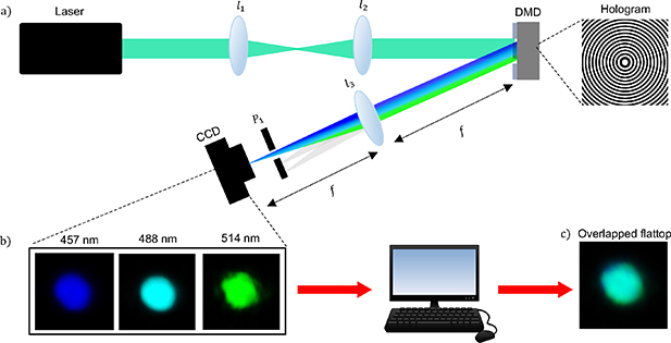
Figure 19. (a) An Argon-ion laser emitted a broadband beam (consisting of λ = 457 nm, 488 nm, 514 nm) and was imaged onto the DMD a telescope with achromatic lenses l1 (f = 100 mm) and l2 (f = 100 mm). The DMD was encoded with a hologram (inset) and Fourier transformed by achromatic lens l3 (f = 200 mm). Before the focal plane, the +1st orders of each wavelength were selected using aperture, P1. (b) CCD camera intensities for each wavelength. (c) The images were then imported as matrices into MatLab where they were converted into their true colour, added together and normalised, for the final digitally overlapped broadband flat-top.
Download figure:
Standard image High-resolution imageA zoom in of the experimental results is shown in figure 20. Figure 20(a) shows the camera images at each wavelength (λ = 457 nm, 488 nm, 514 nm) where the design wavelength was λ0 = 488 nm. Figure 20(b) shows the intensity profile of the broadband flat-top beam generated through digital overlap of the individual flat-tops for each wavelength. Figure 20(c) shows the cross-sectional comparison of the individual flat-tops as well as the digitally recombined broadband (multiline) flat-top beam. Apart from some noise, we see that the desired mode was produced correctly for all wavelengths with the digitally recombined flat-top having a correlation value of 99.2% with theory.
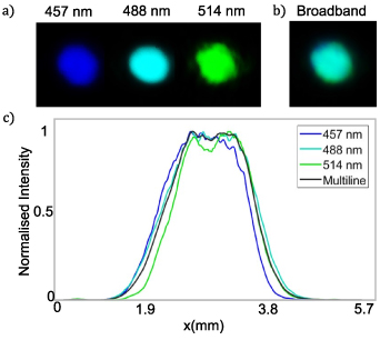
Figure 20. (a) The experimentally generated flat-top beams for each wavelength and (b) the digitally overlapped broadband beam. (c) A cross-sectional comparison of the experimentally generated flat-tops for each discrete wavelength and the digitally recombined multiline beam.
Download figure:
Standard image High-resolution image5.2. Experimental compensation of dispersion
In the previous section we demonstrated that by digitally overlapping each structured beam per wavelength we could achieve a structured broadband beam. The task that now lies before us is to achieve this spatial overlap action experimentally.
In an experimental setting we can recombine the individual structured beams by adding an achromatic lens or achromatic telescope which can be used for single plane recombination as seen in figure 21(a), or we can add a compensating dispersive element, such as a corrective grating (this can be digital or physical) for true collinear beam recombination as seen in figure 21(b). We combine these notions in a typical system as illustrated in figure 21(c), showing the DMD grating as a dispersive element, a telescope that first maps angles to position before recombining them back at an image plane, and an optional second dispersive element (complementary element) to recombine the many wavelengths into a single multi-wavelength outgoing structured beam. This type of configuration is very common in ultrafast laser beam shaping [71, 72]. The options are therefore: (1) if the multi-wavelength beam is needed only at a single plane with full amplitude and phase control, then a simple telescope will work, (2) if only intensity is needed at a single plane then this can be reduced to just one lens, and (3) if the multi-wavelength beam must be collinear and shaped then a telescope and grating pair is needed.

Figure 21. (a) A simple lens or telescope can recombine wavelengths at one plane. (b) A grating can combine wavelengths into a single collinear beam. (c) A combination of both, where an incident broadband beam is wavelength-separated by a grating on the DMD. The dispersed beam is then incident on an achromatic lens placed a focal length distance away from the DMD that maps the angles to positions, with a second achromatic lens recombining the beams at a single plane, the image plane of the DMD. An optional second dispersive element (complementary element) could be used to create a collinear shaped beam. Examples of the outcome are shown using LG beams for (d) just a telescope and (e) telescope and complementary element with an identical grating (physical or digital).
Download figure:
Standard image High-resolution imageThe outcome of this is shown in figure 21(d) for cases (1) and (2): before the image plane the beams disperse, recombine at the image plane, and then separate again after the telescope. Case (3) is illustrated in figure 21(e). By adding a compensating element such as a grating (either a digitally encoded grating or a physical) with the same grating frequency as that grating encoded on the DMD, the dispersion will be exactly counterbalanced, resulting in the individually structured beams travelling collinearly. Hence what we observe in the image plane and thereafter is a single structured broadband beam with the correct phase and intensity profile as seen in the right image of figure 21(e).
Now, let us assume that for a particular application it is only important for the broadband beam to have the desired intensity profile (not the correct phase) in a single-plane. We can then use the simpler recombination method as illustrated in figure 22. The reason why this single lens imaging system recombines the individually structured beams can be understood by referring to basic ray-tracing theory. Although the broadband beam will have the correct structure, it will not have the correct phase because a second element has not been added to correct for the additional phase gained during propagation. After the image plane, the individual beams per wavelength will propagate separately as seen in the right inset of figure 22.

Figure 22. An experimental method for structuring a broadband beam using a DMD and a single lens so that it has the correct intensity at a single plane only. The panels below show the beams at achromatic lens l1 (with focal length f), at the image plane, and after the image plane when the light separates due to propagation.
Download figure:
Standard image High-resolution imageWe demonstrate this method experimentally, with the setup and results shown in figure 23. The setup, illustrated in figure 23(a), follows the experiments already discussed and the reader is referred back to them, with the exception that the achromatic lens l3 (f = 200 mm) is placed in a manner to image the DMD plane. To ensure that the CCD camera was placed in the correct plane it was shifted until a single beam was observed. The results for a LG mode (as an example) are shown in figure 23(b) as camera images, and in figure 23(c) as beam intensity cross-sections. The lower panel of (c) shows the experimental multiline beam and the simulated result, in very good agreement.

Figure 23. Experimental results demonstrating single-plane recombination. (a) The experimental setup consists of a monochromatic broadband beam that has been expanded and collimated by two achromatic lenses l1 (f = 100 mm), l2 (f = 300 mm), where the beam size is controlled by aperture, P1. The beam is then incident on a DMD which has been encoded with a hologram to generate an LG mode. The dispersed beam then propagates to achromatic lens l3 (f = 200 mm) that is located twice the focal length after the DMD. A focal length after the lens a make-shift aperture is placed to select the +1st orders of each wavelength. The beams then propagate a focal length away to the image plane where a CCD camera is placed to observe the single-plane recombined, structured broadband beam; (b) the intensity profiles of each structured LG
 per wavelength, as well as the single-plane broadband beam; (c) the cross-sectional comparison of each structured LG
 mode per wavelength with the broadband beam (above) as well a cross-sectional comparison of the experimentally generated broadband beam and the simulated case (below).
Download figure:
Standard image High-resolution imageThe noise in the recorded beams is worth discussing as it highlights a challenge in these experiments. The noise in the system was as a result of the high grating frequencies used to adequately separate the +1st orders for each wavelength. This was necessary due to: (1) the space limitation, i.e. a large propagation distance to allow the modes to naturally separate was not feasible; (2) the wavelengths are quite close in value, hence when diffracted they do not have a large initial spatial separation; (3) the individual wavelengths and their respective orders were neither evenly spaced nor grouped together, for example, the +1st order of one wavelength could be overlapped with the 0th order of the another wavelength. Due to this effect a make-shift aperture had to be used which was not as efficient at blocking out unwanted modes or stray light as a traditional spatial filter, also contributing to the noise seen in the intensity images. Longer focal lengths and thus longer distances would solve these issues.
Using a second grating produces a collinear beam. This was demonstrated extensively with the use of physical gratings [71, 72] and even more recently in the context of complex-amplitude and phase-only modulation using a DMD [66]. We show an example of the set-up and results of the experiment in [66] in figure 24. As seen in figure 24, the Ti:Sapphire femtosecond laser produced a broadband beam with  [690 nm, 1050 nm]. The physical grating dispersed the broadband beam, with lenses
  expanding and imaging the beam onto the DMD. The DMD, which was encoded with a hologram comprising of a phase mask and an appropriate grating, then structured the incident broadband beam and exactly counteracted the dispersion induced by the physical grating, causing the beam to propagate collinearly thereafter. Lenses
  then expanded and collimated the broadband beam, where the spatial filter F1 was placed in the focal plane of L3 to select the +1st order. To visualise the dispersion angles in the x-plane for each wavelength, the authors then placed a slit after L4 to induce diffraction. Lens L5 was placed thereafter to focus the beam, thus allowing for the +1st order to be selected using spatial filter F2. A 4f-imaging system comprised of
  then relayed this structured mode to the CCD. The authors demonstrated this approach for broadband shaping of Bessel beams, vortex beams and arbitrary images, shown in the insert panels on the right of the figure.

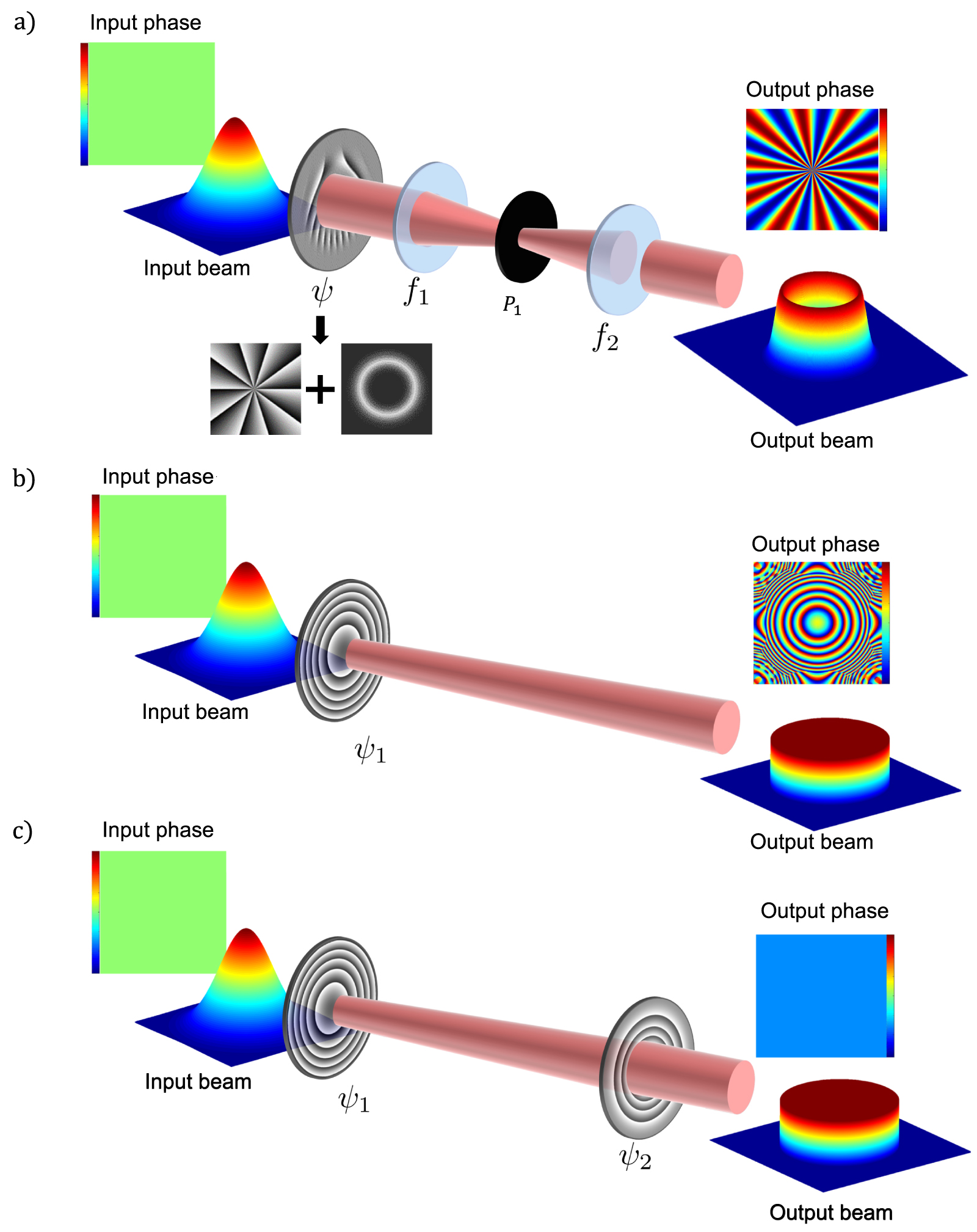
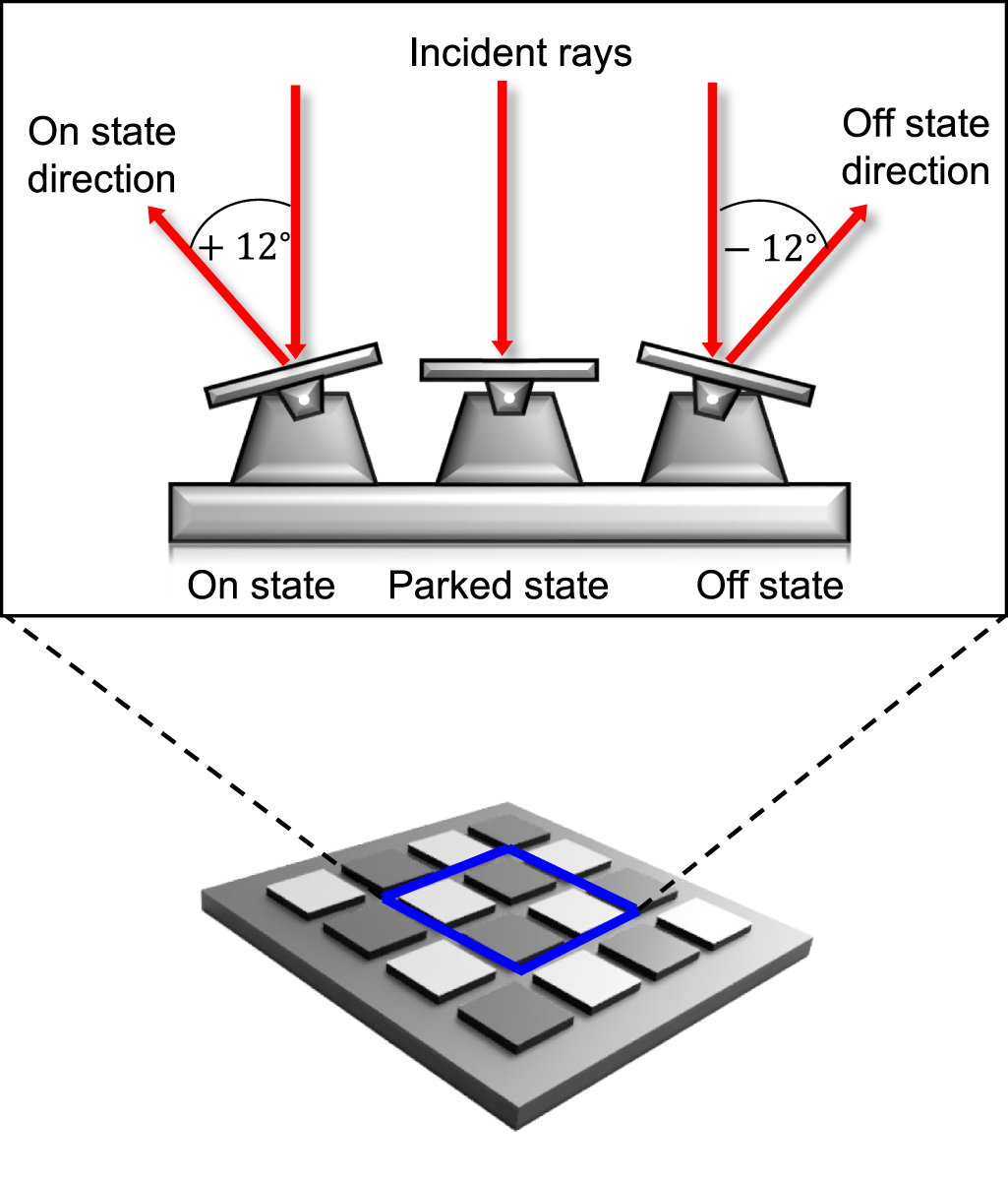
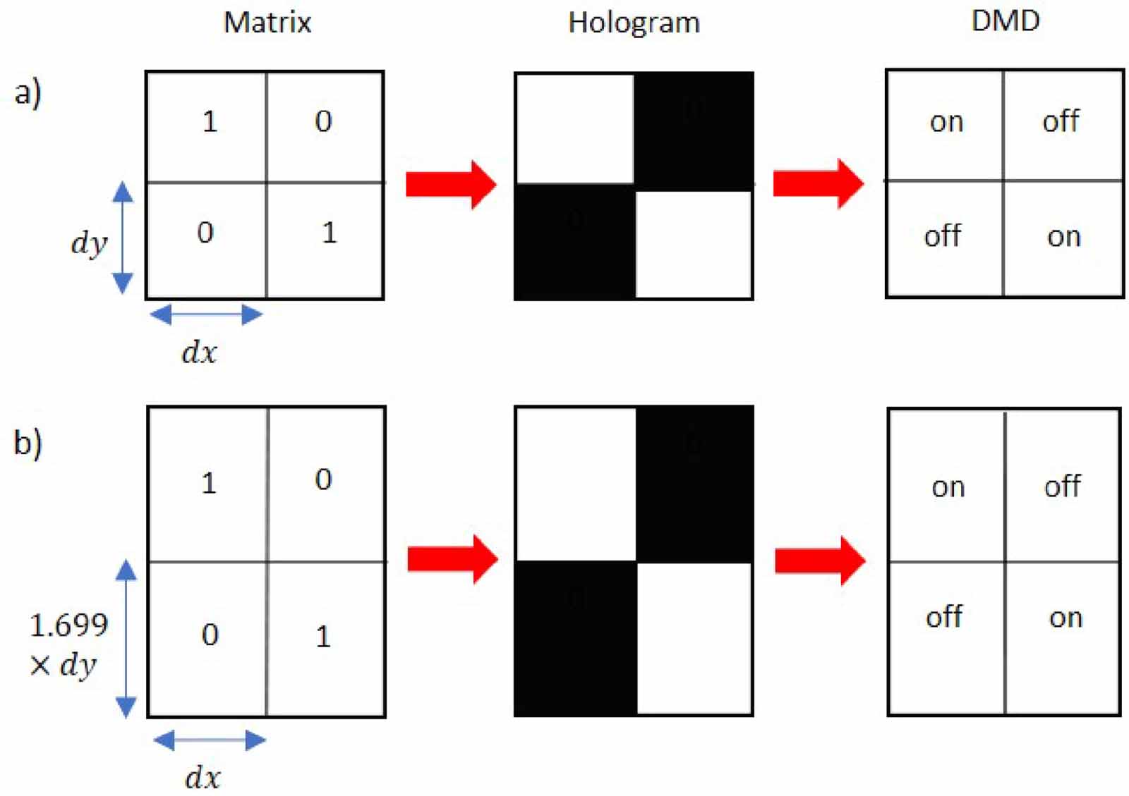
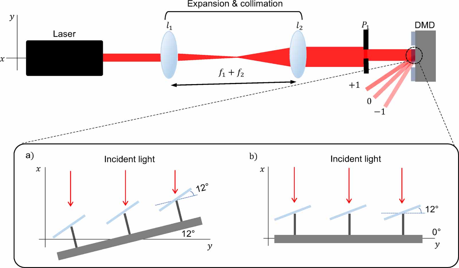
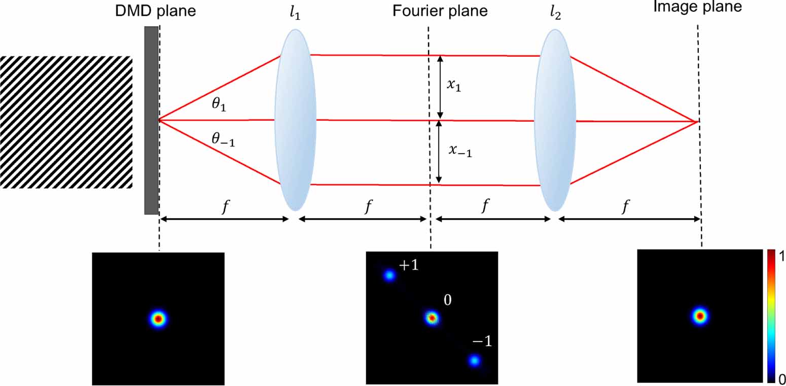
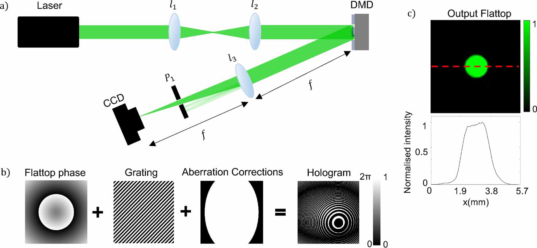
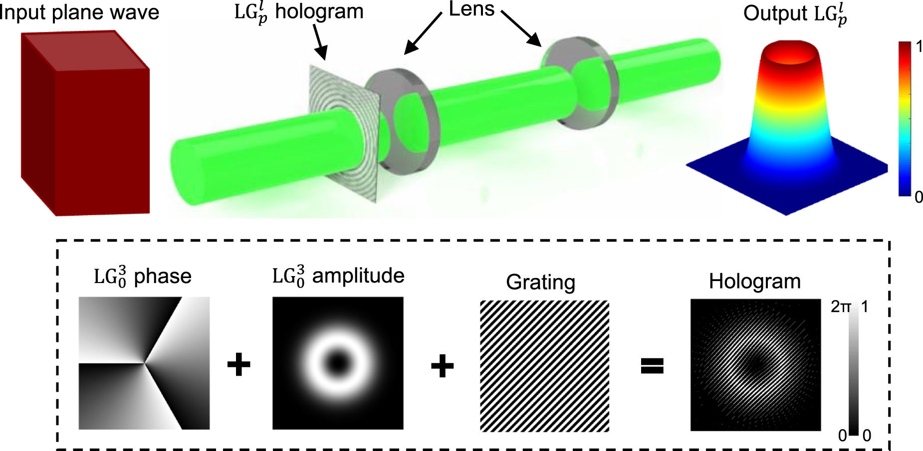
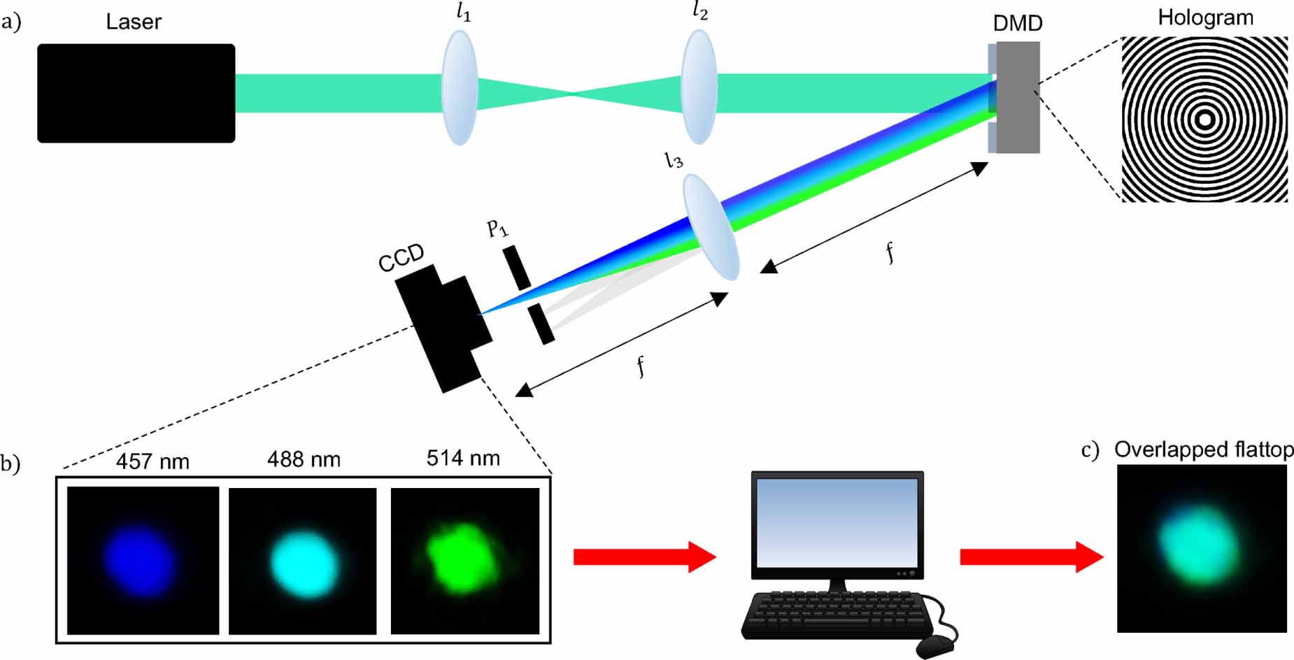
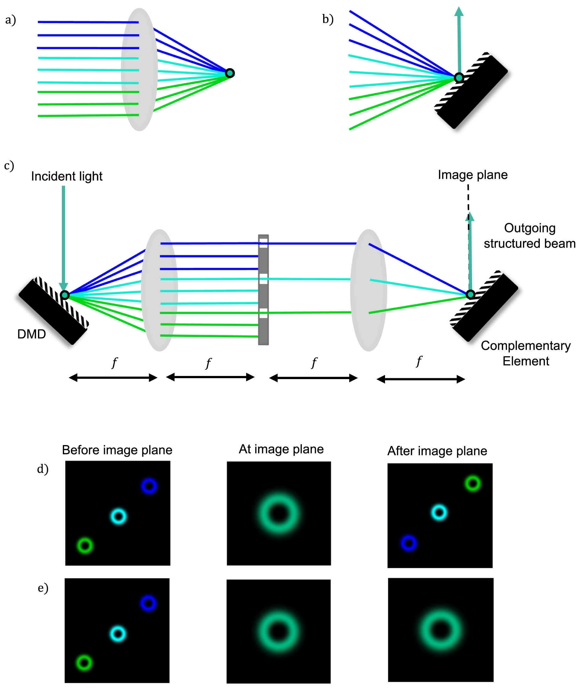
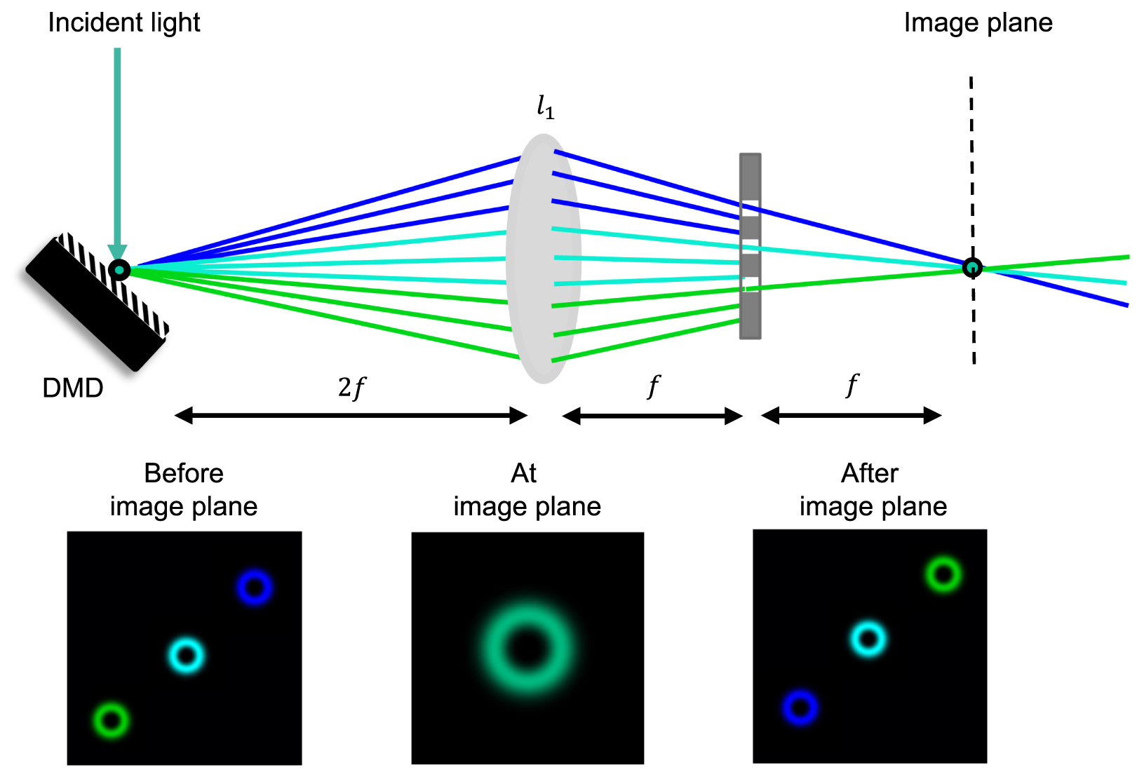
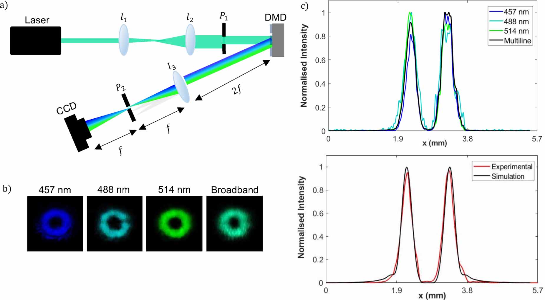
Figure 24. Example of broadband beam shaping with recombination by a grating and DMD pair. The beam panels show experimental results of a Bessel beam (top), vortex (middle) and peace-dove (bottom). Adapted from [66].
Download figure:
Standard image High-resolution image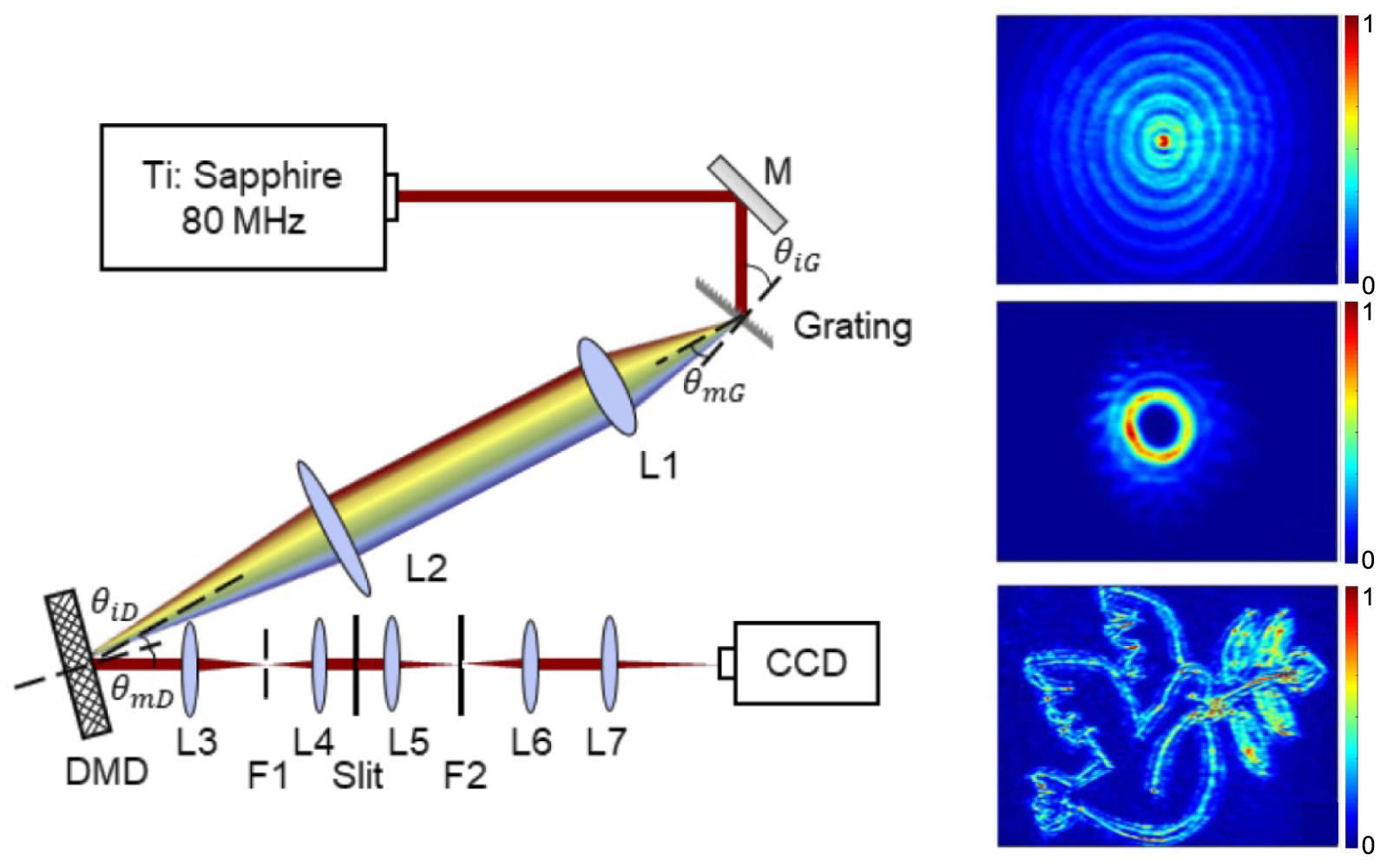
6. Conclusion
In this tutorial we have outlined some useful approaches to getting started with DMDs for shaping light, from monochromatic to broadband sources. We have concentrated on practical issues related to the calculation and implementation of DMD holograms using two exemplary (and topical) case studies, vortex and flat-top beams. We believe that this tutorial will fast track the successful use of DMDs in the laboratory for the creation of novel forms of structured light.
Data availability statement
This is a tutorial with no new data. The data that support the findings of this study are available upon reasonable request from the authors.