Abstract
Analytical forms of the optical helicity and optical chirality of monochromatic Laguerre–Gaussian optical vortex beams are derived up to second order in the paraxial parameter  . We show that input linearly polarised optical vortices which possess no optical chirality, helicity or spin densities can acquire them at the focal plane for values of a beam waist
  via an orbital (OAM) to spin (SAM) angular momentum conversion which is manifest through longitudinal (with respect to the direction of propagation) fields. We place the results into context with respect to the intrinsic and extrinsic nature of SAM and OAM, respectively; the continuity equation which relates the densities of helicity and spin; and the newly coined term 'Kelvin's chirality' which describes the extrinsic, geometrical chirality of structured laser beams. Finally, we compare our work (which agrees with previous studies) to the recent article (Köksal et al 2021 Optics Communications 490 126907) which shows conflicting results, highlighting the importance of including all relevant terms to a given order in the paraxial parameter.
Export citation and abstract BibTeX RIS

Original content from this work may be used under the terms of the Creative Commons Attribution 4.0 license. Any further distribution of this work must maintain attribution to the author(s) and the title of the work, journal citation and DOI.
1. Introduction
A stationary object is chiral if it cannot be superimposed onto its mirror image. Material chirality is a consequence of the geometric position of atoms in molecules and nanostructures. In order to discriminate the chirality of an object in an enantiospecific manner, the probe must also exhibit a chiral structure. Chiroptical and optical activity spectroscopies—using differential light-matter interactions—are widely used techniques to study the structures and functionalities of chiral molecules, biomolecules, metamaterials and nanostructures, as well as achiral objects such as atoms [1–12]. The observables in these spectroscopies are either time-even pseudo scalars or time-odd axial vectors; the former often referred to as true chirality on the account that these effects require chiral material structures, the latter false chirality as they can be supported by achiral media such as atoms as in magnetic circular dichroism [13].
Light most commonly exhibits chirality through circular polarisation (CPL), a local property, where the electric and magnetic field vectors trace out a helical pattern on propagation. The handedness of CPL is denoted by  , often referred to as the helicity, with the positive value corresponding to left-handed CPL, and the negative to right-handed CPL. Less well-known is the fact that light can also possess an additional type of chirality due to its spatial structure, a global property; examples include those stemming from polarisation structure or phase structure [14]. This geometrical chirality of structured light has recently been termed 'Kelvin's chirality' [15]. In this work we are specifically interested in the chirality of beams that possess a phase structure of the form
  where
where  is the azimuthal angle: these modes are often referred to as optical vortices. Analogous to
  for CPL, the sign of the pseudo scalar topological charge
  is what determines the handedness of an optical vortex:
  the vortex is left handed;
  it is right-handed.
Optical vortices have found widespread application since the early 90s—the reader is referred to a few of the many review articles [16–20]—and recently their chirality has been directly utilised in chiroptical spectroscopies [21] and chiral nanostructure fabrication [22].
The conserved pseudo-scalar quantities known as optical helicity and optical chirality (we use lowercase for the local conserved quantity optical chirality of beams; we refer to the geometric chirality of beams as Kelvin's chirality) of electromagnetic fields have found distinct theoretical application in recent years in chiroptical interactions. The optical chirality has been widely studied since Tang and Cohen highlighted its relevance in light-matter interactions [23–32]. For overviews see [33, 34]. Closely related is the optical helicity, which for monochromatic fields is proportional to the optical chirality [35].
In this work we undertake a systematic study of the optical chirality and helicity of optical vortex beams. We begin in section 2 with a brief recap of the general definitions of optical chirality and helicity in free space, followed by giving the necessary quantum electromagnetic mode operators to undertake the calculation of these conserved quantities for Laguerre–Gaussian (LG) optical vortices in section 3. We then derive the analytical formula up to second-order in the paraxial parameter for both circularly polarised and linearly polarised modes in sections 4 and 5, highlighting the particularly interesting case of an optical helicity (chirality) even for linearly polarised modes, as well as the spin-orbit interactions that occur in circularly polarised modes. Furthermore, we comment on a recent study which gives conflicting results to those derived here. In section 6 we look at the spin angular momentum (SAM) density as it is directly linked to the optical helicity through a continuity equation. We conclude with a discussion of the results in section 7.
2. Optical helicity and optical chirality in free space
The most general definitions of the optical helicity  and the optical chirality
  in free space are usually given in terms of the electromagnetic potentials
  and
and  and electromagnetic fields
  and
and  [36]:
[36]:
where  and
and  . Both integrated quantities (1) and (2) are gauge-invariant and Lorentz-covariant, however the integrand of (1) is not gauge-invariant. Throughout this work we deal with gauge invariant integrands at the expense of losing Lorentz-covariance by working within the Coulomb gauge
  and
and  . This is an easily justifiable action in the field of optics. The integrands in (1) and (2) are known respectively as the optical helicity density
  and optical chirality density
  . The introduction of the potential
  ensures that (1) retains its form under duplex transformation [37, 38], i.e. the expressions (1) and (2) are dual symmetric. The necessity of these quantities being dual symmetric is most obvious when one realises, they are conserved for the free field, i.e.
  . Thorough discussions on some of the more fundamental and subtle aspects of the form and properties of (1) and (2) can be found in [33, 34, 39].
We will be using a quantum electrodynamic (QED) formulation in the Coulomb gauge [40] throughout this work, and so the fields and potentials are the microscopic operator versions of those in (1) and (2). Furthermore, compared to numerous studies which utilise natural units  we explicitly use S.I. units. The optical helicity
  may be given in QED as
where 
 is a vector potential operator (see Appendix
  is the transverse electric field operator; and
  is the magnetic field operator. The superscript
  denotes transversality of the field with respect to the Poynting vector in this gauge (not necessarily the direction of propagation);
  is purely transverse irrespective of gauge [40]. The integrand of (3) is the helicity density
  . In the QED theory utilised here we note that (3) does not require the so-called electric helicity contribution
  of (1) necessary in the classical theory to satisfy the conservation law
  . However, it still requires the introduction of the
  in order to satisfy dual symmetry required in the continuity equation with the SAM density
  [36, 37, 41]:

where the quantity  is the correct dual symmetric spin density
  of the free field.
The optical chirality  in QED is defined as
The integrand of (5) is the optical chirality density  . For monochromatic fields the optical helicity (3) and optical chirality (5) are proportional, with the correct proportionality constant being
  as opposed to the routinely reported factor
  due to the more common use of natural units. In this work we study the optical helicity density explicitly as it is a more fundamental quantity, in the knowledge that the optical chirality gives an analogous result for the system we are studying. Due to being in the Coulomb gauge we can re-write (3) in terms of the electromagnetic fields only
where we have used the fact that  and
and  ; both (6) and the spatial integrand of (6) are clearly gauge-invariant. It is highly interesting to note that the expressions (3) and (6) hold in either the standard (asymmetric, electric biased) or dual-symmetric theories, all other conserved quantities, like energy density or angular momentum density, take on different forms in either the asymmetric or and dual symmetric theories [39].
3. Electromagnetic field mode operators
In order to evaluate the quantities  and
and  from the previous section we require the form of the electromagnetic field mode expansion operators
  and
and  . Numerous studies in optics and light-matter interactions assume
  and
and  to be purely transverse to the direction of propagation, which itself exactly coincides with the Poynting vector. This essentially plane-wave description of radiation hides a plethora of novel properties of radiation fields in real world optical and nano optical experiments involving focused or spatially-confined light [42]. In order to strictly satisfy Maxwell's equations no physically realisable radiation field is completely transverse. It was Lax et al [43] who first undertook a systematic study of this issue with respect to paraxial light fields, highlighting how to generate the higher-order fields necessary for a completely correct description of a radiation field. In general, a radiation field consists of a usually dominant zeroth-order transverse component
  (the term most resembling a plane-wave description), plus higher, odd-integer-order
  longitudinal components and even-integer transverse components
  . For example, first-order
  and third-order
  longitudinal fields; second-order transverse fields
  , and so on. The reader is referred to the following further references which discuss this topic [44–47]. Each higher-order field component is weighted by the so-called paraxial factor
  , where
  is the wave number and
  is the beam waist at the focal plane
  , and as such the magnitude of higher-order terms are directly related to the degree of focusing (or confinement).
In this work we specifically concentrate on the LG optical vortex mode, a solution to the paraxial wave equation in cylindrical coordinates. These are the most widely utilised type of optical vortex beam in experiments. The LG mode is characterised by four parameters  : the wave number
  ; polarisation
  ; topological charge
  ; and radial index
  with
with  indicating the number of radial nodes. The zeroth-order electric field
  mode expansion operator
  for a LG mode in the long Rayleigh range
  , where
  , is given by [48]:
where  is the polarisation unit vector for a z-propagating,
  polarised, photon;
  is the annihilation operator;
  is the phase factor, the azimuthal dependent part being responsible for the orbital angular momentum (OAM) of LG modes;
  is a radial distribution function (see appendix
  is the quantisation volume;
  is a normalisation constant; and H.c. stands for Hermitian conjugate. The zeroth-order transverse field (7) gives a realistic physical picture provided
  [49].
[49].
With the aid of Faraday's and Ampere's laws we can calculate the first-order longitudinal  and second-order transverse
  contributions to equation (7), as well as the zeroth and second-order transverse,
  and
and  , respectively, and first-order longitudinal magnetic fields
  . Namely, Faraday's law produces
Then inserting equation (8) into Ampere's Law
Note we could have also used Gauss's law and  to calculate the first-order longitudinal fields, sometimes referred to as the 'transversality conditions of Maxwell's equations'. The explicit forms of the individual contributions
  and
and  for both circular and linear polarisation can be found in appendix
4.
 and
contributions to the optical helicity
and
contributions to the optical helicity


In calculating  with equations (8) and (9) there is the possibility of nine distinct terms:

however it is clear that any cross-terms between longitudinal and transverse components in the dot product will be zero:  and so there are only five terms that require investigation:
The zeroth-order pure term takes on its maximum value for CPL and is zero for linearly polarised inputs. The interest moving beyond this zeroth-order approximation often made is twofold: Firstly, other terms in equation (11) are not necessarily zero even for linearly polarised optical vortices; and secondly that spin-orbit-interactions of light (SOI) occur in optical vortices through higher-order components of the field.
In this section we calculate the helicity density contributions from the pure zeroth-order fields  and the first-order longitudinal fields
  . We give analytical results for the important cases of a circularly polarised input and a linearly polarised input in the
x
-direction but note results are in general polarisation-dependent. In the next section we calculate the
. We give analytical results for the important cases of a circularly polarised input and a linearly polarised input in the
x
-direction but note results are in general polarisation-dependent. In the next section we calculate the  and
and  contributions; we do not calculate the
  term as it significantly smaller than the other terms in general (see section 7).
4.1. Circularly polarised fields
To the level of  and
and  the field mode operators take on the following form for a circularly polarised input [51]
and
Assuming an input monochromatic field mode of  photons and inserting equations (12) and (13) into equation (6) gives an optical helicity density
where we now drop the dependencies of the factors for notational brevity; the forms of  and
and  can be found in the appendix
  of equation (14) gives the expected result of being the difference in number left and right-handed circularly polarised photons.
There are three distinct combinations of  and
and  which lead to differing forms of (14) [52]. When
  (i.e. a Gaussian beam) we yield optical helicity densities in the focal plane which are purely down to the CPL state
  , these are plotted in figure 1. All figures throughout the manuscript correspond to a value of
  and it must be remembered that the phenomena which arise from longitudinal fields and higher-order transverse fields become more substantial the smaller
  becomes.

Figure 1. Normalised optical helicity (chirality) density distribution equation (14) in the focal plane for  for
for  and (a)
  (b)
(b)  . These helicity (chirality) densities stem purely from the pure zeroth-order transverse fields
  .
.
Download figure:
Standard image High-resolution imageThe other two distinct combinations are for parallel  or anti-parallel
  combinations of SAM and OAM. The most interesting examples of the difference in behaviour of these two distinct combinations are for the
  modes, and these are plotted in figure 2 (all figures throughout this work are plotted for
  ). We see that when
  we produce an on-axis optical helicity density in the focal plane, this SOI
  is also responsible for the on-axis intensity of tightly-focused vortex beams [53, 54]. The peak magnitude of this on-axis density due to the longitudinal fields is
  of the absolute maxima stemming from the transverse fields. It is highly important to note however that the relative magnitude between the two is related to the smallness of
  and the tighter the focus the larger the longitudinal field contributions become relative to the transverse ones [51]. The same mechanism is at play for
  —plotted in figure 3—however the effect is much less obvious because the longitudinal term
  responsible for the on-axis density when
  is now
  .
.

Figure 2. Normalised optical helicity (chirality) density distribution equation (14) in the focal plane for  (a)
(a)  (b)
(b)  (c)
(c)  (d)
(d)  .
.  (a)–(d). The helicity densities in (a) and (b) have a major contribution from the zeroth-order transverse fields
  which is
  and a smaller, on-axis contribution from
  (i.e.
(i.e.  ); the helicity densities in (c) and (d) have a major contribution from zeroth-order transverse fields
  that is
  , but the
  contributions in this case are
  . Dashed circles aid visual clarity of the non-zero on-axis helicity density in the cases where
  .
.
Download figure:
Standard image High-resolution image
Figure 3. Normalised optical helicity (chirality) density distribution equation (14) in the focal plane for  (a)
(a)  (b)
(b)  (c)
(c)  (d)
(d)  .
.  (a)–(d). The helicity densities in (a) and (b) have a major contribution from the zeroth-order transverse fields
  which is
  and a smaller contribution from the
  term which produces a helicity density
  ; the helicity densities in (c) and (d) have a major contribution from zeroth-order transverse fields
  but the contribution from
  . Dashed circles aid visual clarity of the
 contribution when
  compared to
  .
.
Download figure:
Standard image High-resolution image4.2. Linearly polarised fields
For a linearly polarised beam in the x -direction the field mode operators take the form;
and
Once again, inserting equations (15) and (16) gives an optical helicity density of a monochromatic beam as
which we see has the correct units of an angular momentum density. The helicity density distribution (17) is shown for  and
and  in figures 4 and 5, respectively. We observe a non-zero optical helicity (and optical chirality) for a linear-polarised electromagnetic field, for the
  case the maximum value is on-axis along the so-called optical vortex core. This feature of optical vortices was first pointed out by Rosales-Guzmán et al for Bessel beams [55] and subsequently experimentally verified for LG beams by Woźniak et al [56]. We return to this result in section 7. A more recent study also looked at the optical chirality and helicity of linearly-polarised LG modes [57] but produced results that do not match our results or the previous studies—we return to this issue in section 5.3.

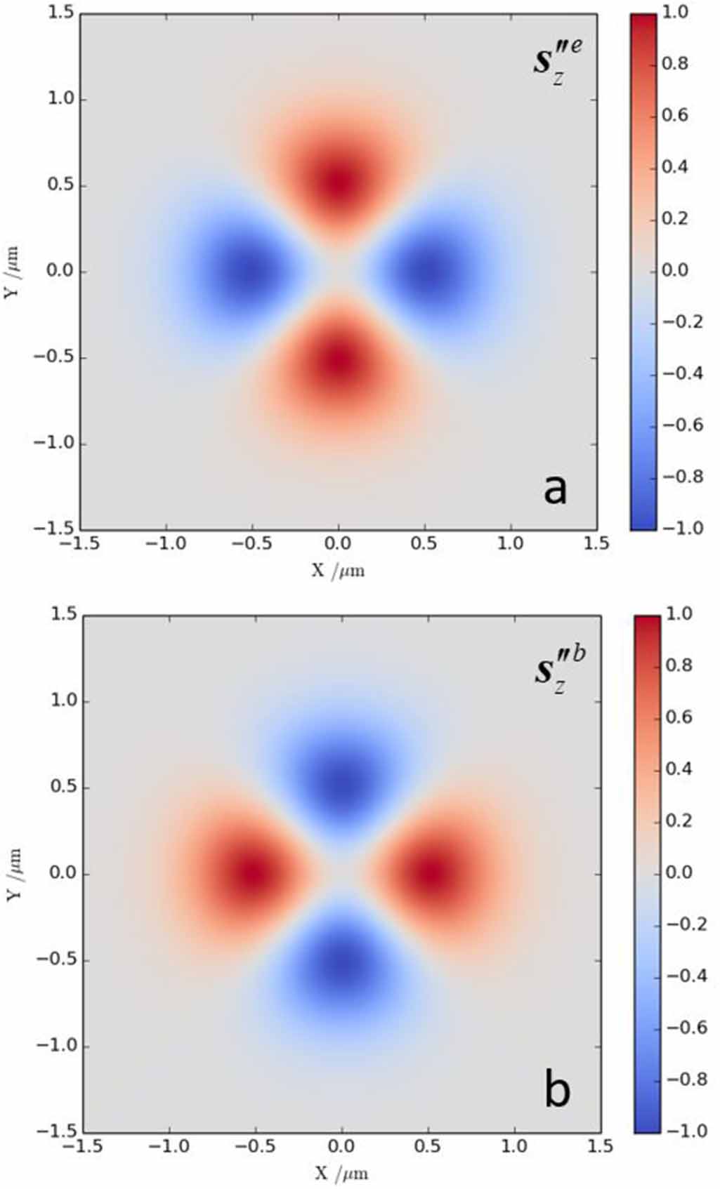
Figure 4. Normalised optical helicity (chirality) density distribution of equation (17) in the focal plane for  (a)
(a)  (b)
(b)  .
.  (a) and (b). These optical helicity densities for linearly polarised vortex beams stem purely from the
  longitudinal fields contribution.
Download figure:
Standard image High-resolution image
Figure 5. Normalised optical helicity (chirality) density distribution equation (17) in the focal plane for  (a)
(a)  (b)
(b)  .
.  (a) and (b). These optical helicity densities for linearly polarised vortex beams stem purely from the
  longitudinal fields contribution.
Download figure:
Standard image High-resolution imageUnlike the optical helicity  of a circularly-polarised monochromatic beam which has a non-zero value, the relevant integral of (17) is zero:
This indicates that particles smaller than the beam waist may probe the optical helicity density (17), but particles which are larger couple to (18) and thus do not exhibit the propensity to engage with the optical helicity generated from OAM in the focal plane.
Sections 4.1 and 4.2 show us that the optical helicity and optical chirality are influenced by OAM. Thus we see that the conclusions of Cole and Andrews [58, 59], i.e. OAM does not influence optical helicity (chirality), are only correct when restricted to the zeroth-order transverse components of the field and is in general not true for optical vortices. Of course, the integrated value  is purely a measure of the number of circularly polarised photons, but the optical helicity (and chirality) densities are significantly influenced by optical OAM of vortex beams. Qualitatively we see the influence of optical OAM on these quantities most dramatically for linearly polarised inputs, however all parameters being the same we quantitatively see that for the circularly polarised input the peak on-axis magnitude is twice that of the linearly polarised case for
  [52].
[52].
5.
Contributions involving the second-order
transverse fields

When looking at equation (11) the terms  and
and  are theoretically of the same magnitude as the
  term of the previous section. As such, their contributions should also be calculated and taken account of. Similarly, we carry out this analysis for a circular- and linearly polarised input LG mode.
5.1. Circularly polarised fields
The electromagnetic field mode expansions operators now include the  components necessary to computer the second-order transverse components to the optical helicity and chirality. For circularly polarised fields they take the form
and
Inserting equations (19) and (20) into (6) and after some tedious algebra we produce
where we have specifically labelled what parts can be attributed to what order fields. We see equation (21) has the correct units of an angular momentum density. The difference between equations (21) and (14) is that the former includes the  components and in figure 6 the radial distributions of the optical helicity for both has been plotted against one another, highlighting that including
  does not affect the on-axis optical helicity of
  beams, but adds quantitative corrections to the transverse spatial distributions.

Figure 6. Normalised optical helicity (chirality) density distributions for equation (21) in the focal plane which includes  contributions
  (a)
(a)  (b)
(b)  .
.  . Note that the solid lines are the line plots of the transverse spatial distributions in figures 1–3 which include contributions from only
  and
and  , and we see that inclusion of the second order transverse fields
  only influence the optical helicity densities
  around the peak magnitude quantitatively; the SOI contributions
  to the densities are unaffected by inclusion of
  .
.
Download figure:
Standard image High-resolution image5.2. Linearly polarised fields
The electromagnetic field mode expansions operators including the  components for linearly polarised in the
x
-direction inputs are
components for linearly polarised in the
x
-direction inputs are
and
The optical helicity density is
We see that including second-order transverse fields to the order of  does not affect the optical helicity (chirality) of a linearly polarised optical vortex because
which put back into equation (24) gives the same result as equation (17) which was derived by including only the zeroth-order transverse and first-order longitudinal components of the field: the optical helicity (and optical chirality) that stems from the OAM is manifest purely through longitudinal components of the field. Furthermore, whilst the helicity associated with circular-polarisation of transverse fields correlates to a spin density in the direction of propagation, we see that the helicity associated with longitudinal fields is related to the transverse spin density [60, 61] (see section 6).
5.3. Comment on Köksal et al study
A recent study by Köksal et al [57] (also see [62]) examined the optical chirality and helicity for monochromatic linearly polarised (in the
x
-direction) LG beams in free space. However, although an identical system to ours, their results conflict with those given here, as well as those in previous studies [52, 55, 56]. In their work they addressed why their results differ from those given in [56] specifically, suggesting that because the light is focused by a lens in the experiment this alters the optical chirality and helicity and their theory does not account for influence of the lens apparatus. However, in this study we have not considered the act of any experimental apparatus explicitly and our results fully agree with previous theory and qualitatively with experiment. In fact, both Köksal et al and the work here relies on the magnitude of the paraxial factor  , i.e. the ratio of wavelength to beam waist, which essentially accounts for focusing. The reason why the Köksal et al study does not produce the same results as other studies and here is that they do not include all the necessary terms in their calculations. Specifically, in their study they include the
  terms of equation (11) but have neglected the term
  . If we go back to our calculations and neglect the same term Köksal et al do then we produce the following optical chirality density
where the first three terms in square brackets stem from the transverse fields and the final term is that from the longitudinal contribution. Plotting equation (26) for  produces (see figure 7) qualitatively the same optical chirality density distributions in the focal plane as given in figure 2 in the paper by Köksal et al. We note that our minima are not the same absolute magnitude as our maxima as is the case in Köksal et al.
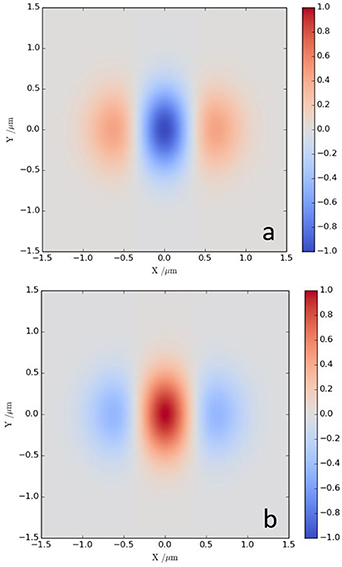
Figure 7. Plot of equation (26) which produces the same optical chirality density (qualitatively—see main text) in the focal plane as the Köksal et al study (figure 2 of [57]). (a)  (b)
(b)  .
.
Download figure:
Standard image High-resolution imageThe term  neglected by Köksal et al is given explicitly as
which when added to equation (26) gives the circularly-symmetric
and is essentially what is given in equation (24) besides the factor of  , i.e.
  , with the corresponding circular-symmetric optical chirality distributions of figures 4 and 5. As such, by including the term
  we produce the expected result.
The origin of the importance of including all the necessary terms is that the electric and magnetic fields of radiation fields do not necessarily contribute equally to conserved quantities in free space. What we observe here is that  for a linear polarised field, however this does not suggest that we require a specific dual-symmetric equation to calculate the helicity and chirality: as noted in section 2 the equation for optical helicity and chirality is identical in both symmetric and asymmetric formulations [39] (The helicity and optical chirality are unique quantities in this respect for the free field). Rather all terms must be included up to a given order of the paraxial parameter. Optical helicity and optical chirality are in fact particularly unique as unlike other quantities (canonical momentum density, spin momentum density, energy density, etc) which engage with the electric biased nature of materials in actual experiments (generally), optical helicity and optical chirality specifically couple to chiral matter via electric and magnetic dipoles, and so this is why the experiment produces the circularly-symmetric helicity rather than the electric biased result (26).
6. SAM density
As mentioned in section 2, there is a continuity equation (4) which relates helicity to spin. The SAM density  is given explicitly in coulomb gauge QED as
As shown for the optical helicity and chirality, the spin density can similarly be calculated to an  th order in the paraxial parameter:
Unlike the optical helicity and chirality (as well as energy density, for example) which progress in  degrees of the paraxial parameter (see equation (11)) the SAM density involves
  contributions. The zeroth-order term
  is zero for linearly polarised beams, and its integral value takes on values of
  per photon in the direction of propagation for CPL. The first-order contribution is responsible for transverse spin density [60, 61, 63], calculated with our QED mode expansions as:
where  is the magnetic field contribution and
  is the electric field contribution [64]. The individual
  and
and  , as well as the total
  , parts of equation (31) are plotted in figure 8 for
  .
.

Figure 8. Components of transverse SAM density (a)  term in equation (31); (b)
  term in equation (31); and (c) the total
  equation (31).
  for (a)–(c).
Download figure:
Standard image High-resolution imageThe second order contribution using QED mode expansions is:
Remarkably what this shows is that there exists a SAM density in the direction of propagation even for linearly polarised input optical vortices [65–67]. Note that each term in (32) is dependent on  and so this phenomena is unique to optical vortices: a linearly polarised Gaussian beam
  does not possess this longitudinal SAM density. The total dual symmetric contribution (32) is actually zero due to equation (25), however experimentally of course light-matter interactions are generally dominated by electric dipole coupling and so the electric field contribution to equation (32) should be observable provided
  is small enough. The individual electric
  and magnetic
  contributions of equation (32) are plotted in figure 9.

Figure 9. Components of longitudinal SAM density of (a)  term in equation (32); (b)
  term in equation (32)
  ,
,  for (a) and (b).
Download figure:
Standard image High-resolution imageAlthough the optical helicity was calculated using the formula (6), another way is to calculate the projection of the spin onto the linear momentum density  , where
  is the (orbital) canonical momentum density, calculated in paraxial form as
It is easily seen that projecting equation (31) on to equation (33) gives the correct helicity density (17) which was calculated using the integrand of (3). The helicities associated with the second order spin density (32) are
The sum of these two contributions (which is obviously zero) to the optical helicity density correspond to those terms calculated in equation (24) which are zero. The relevance of these two contributions to the helicity (34) and (35) individually are not important as we have stated the material response to helicity is not electric biased and so the individual non-zero (34) and (35) cannot be observed experimentally.
7. Discussion and conclusion
We now discuss in more detail the specific result equation (17). What this tells us is that linearly-polarised optical vortices with small beam waists on the order of the input wavelength  acquire a significant optical helicity and chirality density in the focal plane, even though they possess no spin, helicity, or chirality before focusing (i.e. when
  ). Clearly CPL and helicity (chirality) are not synonymous. This phenomena is a spin–orbit-interaction of light (SOI) [53], but in contrast to the very well-known spin-to-orbital angular momentum conversion, this mechanism is an orbital-to-spin angular momentum density conversion. Whilst SAM-OAM conversions are very well-known and studied, the OAM-SAM conversion process has only recently seen a large degree of research activity, and these studies are have been interested in the corresponding spin-angular momentum density (section 6) generation from OAM which leads to mechanical effects on matter [65, 66, 68–73] (rather than the corresponding optical helicity and chirality density generation we have been interested in, which relate to spectroscopic light–matter interactions). The OAM-SAM conversion is more obvious to recognise by recalling the continuity equation (4): a degree of helicity density is produced (equation (17)) which is accompanied by a generation SAM density
  . We obtain this same result by calculating
  to begin with and then calculating the corresponding helicity density generation (section 6). A very important point to note however is that the quantities
  and
and  are local and intrinsic, being linked to light's polarisation. The presence of
  in equation (17) and many other equations throughout this work suggest the ability of optical vortices to engage in chiroptical interactions with matter via the handedness/chirality of an optical vortex. More strictly, the handedness of the optical vortex determines the sign of the quantities
  and
and  , and it is these quantities which play the role in light-matter interactions. As such, chiral matter may indirectly show a discriminatory response to the pseudoscalar
  [21, 52, 56].
This still leaves the question to whether the actual spatial (i.e. geometrical) chirality of optical vortices influences spectroscopic light-matter interactions directly through the sign of  . This has been a question researchers have been asking for quite some time now [21, 74], and very recently Nechayev et al [15] introduced the term 'Kelvin's Chirality' to describe this geometrical chirality that may be possessed by structured light beams, a property seemingly quite distinct from the local properties (with the introduction of Kelvin's chirality of optical beams, it may be necessary in future to refer to the distinctly different optical chirality studied in this article as 'Lipkin's chirality'). A QED study [75] highlighted how electric quadrupole couplings are essential for chiral particles to engage with the Kelvin's chirality of optical vortices (via electric-dipole electric-quadrupole interferences), the reason being they interact with the transverse gradient of the field (even in the paraxial approximation, i.e. zeroth-order transverse field components only), of which the helical part is what gives vortices their OAM of
  . This initial study was specifically concerned with dichroic-like absorption of optical vortices, and further studies have highlighted this dependence on
  in both linear [76] and nonlinear [77] scattering optical activities via electric quadrupole couplings. The fact that OAM of optical vortices is transferred to electronic degrees of freedom via electric quadrupole couplings (to leading order) in bound electrons agrees with these results [78]. However, without focusing (or spatial confinement of the fields) such effects are essentially still relatively small compared to those dependent on the longitudinal phase gradient associated with the wavelength, due to the fact Kelvin's chirality of these beams is a global property of the beam directly proportional to the beam waist
  . Indeed, the relatively large helical pitch of circularly-polarised light (related to the wavelength) is one of the reasons why chiroptical interactions in small chiral particles are generally small in the first place; the pitch of an optical vortex is
  . A recent experimental study strikingly highlighted the scale-dependent nature of Kelvin's chirality by matching the size of chiral microstructures to that of the optical vortex beam waist [79]. Furthermore, although one can picture the azimuthal phase of an optical vortex tracing out a helical path on propagation, there is no optical helicity associated with this property of electromagnetic beams as can easily been seen by projecting the OAM onto the linear momentum [74, 80].
We now conclude with a summary of the key results from this work:
- Linearly polarised optical vortices possess significant optical helicity and chirality densities for values of the beam waist which stems purely from first-order longitudinal fields. This is a local OAM-SAM conversion.
- Circularly polarised optical vortices have increased optical helicity and chirality densities when via a spin-orbit interaction and this also comes from first-order longitudinal fields.
- Because all of the main quantities in this work depend on the first-order longitudinal fields they are proportional to the smallness of the paraxial parameter and their magnitude increases the tighter the focus.
- The continuity equation between spin and helicity densities tells us that the helicity associated with linearly polarised vortices relates to the extraordinary polarisation-independent transverse spin momentum density.
- Even for linearly polarised optical vortices there exists a spin momentum density in the direction of propagation (figure 9), and this does not exist for non-vortex Gaussian modes.
- When calculating conserved quantities that depend on both electric and magnetic fields, the inclusion of every term up to the same order of paraxial parameter is essential to obtain correct results.


It also worth commenting on the fact a recent review article [81] has stated measuring both the electric and magnetic fields of a spin–orbit-interaction of light simultaneously would be 'aspirational'—however in [56] this was achieved, and the work here provides the theory behind it.
Finally, we comment on the fact we neglect the terms proportional to  in equation (11) as only in the most extreme cases of subwavelength focusing could these become important. It must be noted that inclusion of those terms would also then require
  and
and  to be included also. It can be predicted that an on axis optical chirality and helicity density would be produced by these higher-order terms when
  due to the on-axis intensity which is known to exist in this regime [54].
Acknowledgments
K A F is grateful to the Leverhulme Trust for funding him through a Leverhulme Trust Early Career Fellowship (Grant Numbers ECF-2019-398). We thank David L Andrews for helpful comments.
Data availability statement
No new data were created or analysed in this study.
Appendix A.: Radial distribution function
The radial distribution function  is
is
where the normalisation constant is given by ![$C_p^{\left| \ell \right|} = \sqrt {\frac{{2p!}}{{\left[ {\pi \left( {p + \left| \ell \right|} \right)!} \right]}}} $](https://content.cld.iop.org/journals/2040-8986/23/11/115401/revision2/joptac24bdieqn254.gif) and
and  is the generalised Laguerre polynomial of order p. The
  case is most experimentally utilised (and corresponds to all the figures plotted in this paper), and the differentiations from the main manuscript are given analytically in this case as
More generally
Appendix B.: T0 Electromagnetic vector potentials
The zeroth-order transverse electromagnetic vector potential mode expansions for LG beams are given as
where  , thus

Appendix C.: Explicit forms of transverse and longitudinal field components (up to second order in the paraxial parameter)
For circularly polarised light
For linearly polarised (in the x direction) light