
Abstract
Free-space laser communication (FSLC) has attracted wide attention and developed rapidly due to its high bandwidth and strong capability to resist interception and interference. However, communication performance is severely affected by atmospheric turbulence. In this paper we consider the end face of the coupling fiber and adopted power-in-the-bucket (PIB) as the evaluation criterion instead of the traditionally used coupling efficiency. The relationship between FSLC performance (PIB) and adaptive optics parameters (corrected Zernike modes number) is derived for the first time. We simulated and conducted an 8.9 km horizontal FSLC experiment to analyze the effects of corrected modes on communication performance. The simulation and experiment results consistently show that, for turbulence of r0 = 7.51 cm, it is sufficient to correct the first 30 modes. The bit error rate (BER) and the PIB reached values of about 10−7 and 70%, respectively. For r0 = 4.43 cm correction of the first 22 modes, yielded BER and PIB values of around 10−5 and 55%, respectively. For r0 = 1.7 cm, no matter how many Zernike modes are corrected, the BER and PIB values are about 10−3 and 20% respectively. This experiment and its results provide an important reference for corrected modes on communication performance under different turbulence strengths.
Export citation and abstract BibTeX RIS

Original content from this work may be used under the terms of the Creative Commons Attribution 4.0 license. Any further distribution of this work must maintain attribution to the author(s) and the title of the work, journal citation and DOI.
1. Introduction
With the rapid development of technology, wireless communication has played an important role in our daily life. Since traditional microwave communications are hard to complete at transmission rates greater than 1 Gbps [1], this approach is gradually becoming insufficient to meet our demands. Free-space laser communication (FSLC) has emerged as a potential solution due to its high bandwidth, anti-interference performance [2–6], and high communication speed [7]. However, FSLC is more easily influenced by atmospheric turbulence than microwave communication due to the shorter wavelengths used in FSLC.
An adaptive optics (AO) system can compensate for the wave front distortion induced by atmospheric turbulence, thereby improving communication performance. Much of the existing research focuses on improving communication by AO systems. For satellite-to-earth communication links, Chen et al analyzed the influence of the atmosphere on coupling efficiency (CE) and conducted 2.5 Gbps laser communication experiments based on AO, which confirmed that AO systems can increase average received power and reduce average bit error rate (BER) [8]. Wright et al demonstrated an optical downlink from the International Space Station to the Optical Communications Telescope Laboratory at the Table Mountain Observatory, California. The results of this experiment indicated that the Strehl ratio improved from less than 0.02 to about 0.6 and that the coupled power was improved by 16 dB after correction by an AO system [9]. In terms of the horizontal link, there are fewer experimental reports on FSLC with AO. Weyrauch and Vorontsov investigated wave front control by using the stochastic parallel gradient descent micro-electro-mechanical systems adaptive system operating on a 2.33 km near-horizontal atmospheric propagation path using partially coherent extended beacons in 2005 [10]. For the impact of Zernike modes on communication performance in horizontal links, Liu et al [11] simulated the performance improvements on atmospheric coherent laser communications after correcting different numbers of Zernike modes with AO. Wang et al [12] performed an indoor experiment and analyzed the influence of different Zernike modes on CE. As the CE cannot precisely evaluate the receiving energy efficiency affected by an AO system, our group instead proposed the power-in-the-bucket (PIB) method [13]. Wang et al [14] conducted an outdoor experiment and analyzed the effect of the bandwidth of an AO system for horizontal FSLC using the PIB method, however, to date, there is still no outdoor experimental research on the effect of Zernike modes on horizontal FSLC with PIB.
In this paper, we studied the quantitative relationship between the number of corrected Zernike modes (i.e. spatial characters of aberrations) and communication performance (PIB and BER). The influence of different spatial frequency aberrations on the performance of FSLC can then be obtained to ensure a basic communication performance. We also conducted an outdoor experiment under different strengths of turbulence over an 8.9 km horizontal distance. From the theoretical and experimental results, we expected to analyze: (a) if the experimental results show overall consistency with the theoretical results and (b) the corrected mode numbers needed for basic communication performance under different turbulence strengths. As the selection of the deformable mirror (DM) and the design of the Shack–Hartmann wave front sensor (S–H WFS) in the AO system are based on the spatial characteristics of the aberrations, such findings would be of significant guidance for the practical application of AO systems used in FSLC systems.
2. Theory
2.1. The PIB of FSLC systems
The standard practice for coupling power evaluation is the use CE, which is an important parameter in a FSLC system that determines the light power that can be detected in the fiber. The calculation of CE is based on the optical field distributions of the signal beam at the fiber end face and the optical fiber mode. The fundamental mode of power distribution in a fiber can be approximated within a 1% error in a Gaussian beam if the normalized frequency V of the optical fiber is in the range 1.9 < V < 2.4. Based on this condition, the Gaussian approximation can be used to describe the optical fiber mode field distribution characteristics. However, CE cannot accurately describe the energy in the actual fiber, especially for strong turbulence, and moreover, CE ignores the area of the laser-receiving end face, which leads to further inaccuracy in the approximation. PIB not only takes into account the optical field distribution of the beam, but also the size of the fiber end face when calculating the energy receiving efficiency. Thus, in this paper, we adopt the PIB as a more accurate evaluation methodology by which to calculate the coupling power [13].
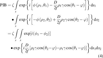
As is shown in figure 1, an incident beam is focused on the surface of the coupling fiber with a coupling lens. The diameter and focal length of the coupling lens are denoted D and f, respectively. The radius of the coupling fiber is R. The entrance pupil and its focal planes are expressed in polar coordinates (ρ, θ) and (γ, ϕ), respectively.

Figure 1. Schematic of the PIB in an FSLC system.
Download figure:
Standard image High-resolution imageThe power coupled into the single mode fiber is:

where I(P) is the received light intensity of point P on the focal plane and  is the end face area of the fiber. According to the Huygens–Fresnel principle, the light intensity of point
  can be described by [15]:

where U[P(γ, ϕ)] represents the complex amplitude of point P:

After substituting equations (2) and (3) into equation (1), the equation for the PIB becomes:
where  ,
,  represents the phase of point (ρ, θ) on the entrance pupil.
Theoretically, PIB can be calculated by equation (4), however, it is challenging to analyze the influence of PIB caused by turbulence. According to Yin's study, the statistical average PIB can be simplified into [13]:

The formula above represents the autocorrelation of the phase in the entrance pupil, where J1(x) is the first-order Bessel function and  is the distance between points ρ1 and ρ2,
Φ is the distorted wave front. Generally, the wave front distortion Φ can be described using Zernike modes. As the number of Zernike modes increases, the spatial frequency of the distortion also increases. The wave front distortion can be described by the linear accumulation of all Zernike modes
is the distance between points ρ1 and ρ2,
Φ is the distorted wave front. Generally, the wave front distortion Φ can be described using Zernike modes. As the number of Zernike modes increases, the spatial frequency of the distortion also increases. The wave front distortion can be described by the linear accumulation of all Zernike modes  . According to Robert J Noll's study, the low order Zernike modes occupy most of the wave front distortion, the higher the order of Zernike mode, the smaller the proportion of the wave front distortion [15]. Hence, the choice of corrected number of Zernike modes used in this study is from low order to high order based on Noll's theory. Thus, we can obtain the theoretical <PIB> with a measured wave front phase of
  after the first J Zernike modes are corrected. The normalized PIB may be written as:
To calculate the mean PIB after correction of different Zernike modes by the AO system, it is essential to find the relationship between the mean PIB and the correct modes  . According to Noll's study [15], if the first J modes are corrected, the remainder of the wave-front distortion can be expressed as:

where  and
and  denote the distorted wave-front and the correction, respectively. Thus, we can calculate the mean square residual error:

The first ten values of  are shown in table 1.
Table 1. Residual error after correction of the first ten Zernike modes.
|
|

|

|
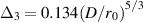
|

|
|
|
|

|
When J is large (J > 10), equation (8) can be approximately by [15]:

Theoretically, we can calculate the PIB with equations (5) and (9) (or table 1), however due to ignoring the fitting error of the DM, the mean square residual error  deduced by Noll idealized result. Hence, to obtain an accurate result, we also must take into account the fitting error.
Considering the fitting error, Védrenne et al studied the mean square residual error of the first  orders after correction by the AO system, which can be expressed by [16]:

So, the mean square residual error after correcting the first  orders is:

This equation considers both the spatial distribution characteristics of atmospheric distortion and the fitting error of the DM, which can more accurately describe the effect of AO correction. Theoretically, based on equations (5) and (11), we can get the PIB after correction of the first J Zernike modes. The choice of AO parameters is based on the communication performance, which is described by BER. Different application scenarios have different requirements for BER. For example, video communication requires BER to be lower than 10−7, audio requires a minimum BER of 10−6 and a value of 10−5 is required for basic communication performance. It is, therefore, crucial to establish the relationship between BER and PIB, so that, we can obtain the relationship between the corrected number J of Zernike modes and BER.
2.2. The BER of FSLC systems
To establish the connection between AO parameters J and communication performance, the BER is essential. The average BER can be obtained from the communication energy, thus the BER can be calculated from the average PIB. If we assume the 'zero' bit and 'one' bit are uncorrelated, the optimal reception BER of homenergic binary code can be expressed as:

where SNR is the signal-to-noise ratio,  is the energy of noise, and erfc() is the complementary error function. Which can be written as:

For an FSLC system, we can determine the effect of turbulence on the BER. By combining equation (5) with equation (12), we can obtain the relationship between BER and turbulence, then shows that turbulence increases BER by decreasing communication energy PIB, and the noise n0 remains unchanged. The BER of fiber optical communication is approximately 10−9, and PIB/2n0 is approximately 36 according to equations (12) and (13). Thus, when using the fiber to receive the laser, the BER as a function of PIB may be written as [13]:

The BER represented by logarithm is near linear to normalized PIB, so the following approximate formula can be used:

where N is the index of BER, i.e.:

Via equation (16), the BER value can be calculated after the first J Zernike modes are corrected by the AO system. Generally, when the BER is lower than 10−5, the basic communication performance can be maintained, hence, the PIB should be larger than 50% according to equation (14).
3. Experiment and results analysis
Although we have deduced the relationship between theoretical PIB (and BER) and corrected modes J so far, we still do not know if realistic PIB (and BER) values are consistent with theoretical expectations. Hence, an outdoor experiment was performed to validate our theoretical analysis above.
3.1. Experiment background
As shown in figure 2, the FSLC experiment was conducted with an AO system from one mountaintop to another mountaintop via a horizontal optical link. An 808 nm laser used as a beacon beam and a 1550 nm laser used as a signal beam are emitted by a transmitting terminal from a mountaintop and are received at a receiving terminal located on another mountaintop. The optical link spans a range of 8.9 km at an average altitude of about 110–202 m above sea level.

Figure 2. Schematic of experiment background.
Download figure:
Standard image High-resolution imageFigure 3(a) shows the schematic diagram and the optical setup of the AO system for FSLC. The lasers of 1550 and 808 nm are used as signal and beacon lights, respectively, and are first received by a telescope with an aperture of 150 mm before entering the AO system. The beam is collimated and reflected by a tip–tilt mirror (TTM) and a DM prior to entering beam splitter SW1, which is designed to reflect 80% of incident 808 nm beams and transmit light of 1550 nm and 20% of light of 808 nm. The reflected light of wavelength 808 nm enters the S–H WFS for wave front detection, and the transmitted light is split again by beam splitter SW2 for TTM tracking. The transmitted 1550 nm signal light is coupled into a fiber, and the reflected light with a wavelength of 808 nm is received by a tracking camera. In this AO system, a 145-element continuous surface DM is used to correct high-order aberration. The diameter of the DM is 25 mm, the stroke of the actuators is 3 μm, and the number of effective actuators is 97. The distorted wave-front is detected by a 15 × 15 S–H WFS with a high speed camera at 1.6 kHz frame frequency with a pixel size of 25 μm. The diameter of the S–H WFS is 2.25 mm. The aperture and focal length of the micro-lens are 3.19 mm and 150 μm, respectively. The TTM (FSM-300, Newport) with a tip–tilt angle of ±1.5° and a 25.4 mm aperture is used to correct tip–tilt aberrations. A tracking camera (EoSens GE, Mikrotron) is used to obtain the tracking error with a region of interest area of 90 × 90 pixels and a frame frequency of 500 Hz. Figure 3(b) shows the actual optical configuration of the designed AO system.
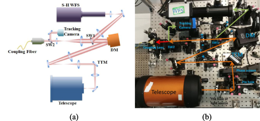
Figure 3. Optical layout of the FSLC AO system (a) schematic diagram (b) experimental setup.
Download figure:
Standard image High-resolution image3.2. Experiment results
In this study, we made a series of experiments under different atmospheric coherence lengths (r0) and conducted the experiment at noon, nightfall and night, at which the representative atmospheric coherence lengths are 1.70, 4.43, and 7.51 cm respectively. In this paper, we corrected the first 65 Zernike modes to test the performance of our AO system.
As is shown in figure 4, we calculated and obtained the theoretical and experimental RMS of the distorted wave front after the first J Zernike modes were corrected. By comparing the theoretical and experimental RMS curves, we can find that the theoretical curve dropped to an ideal level (RMS = 0.05 rad) after correcting the tip and tilt. Experimentally, for the conditions of r0 = 4.43 cm and r0 = 7.51 cm, after correcting the first 11 Zernike modes, the measured RMS value dropped to about 0.05 rad and maintained a stable state. As turbulence becomes stronger (r0 = 1.7 cm), the experimental RMS remains large (about 0.35 rad) even after correcting the first 65 Zernike modes.

Figure 4. (a) Theoretical and (b) experimental root mean square error (RMS) variation curve with corrected modes.
Download figure:
Standard image High-resolution imageAccording to equation (6), we can calculate the PIB after correcting the first J Zernike modes with a measured wave front. Figure 5 indicated the relationship between PIB (theoretical and actual) and corrected Zernike modes. Theoretically, the PIB can reach about 70% for r0 = 4.43 cm and r0 = 7.51 cm after correcting the first 22 Zernike modes. When r0 = 1.7 cm, the PIB reached 60% after correcting the first 22 Zernike modes. In the experimental measurements, due to the influence of turbulence, the PIB reached 70% after correcting the first 30 Zernike modes for r0 = 7.51 cm. When r0 = 4.43 cm, the PIB reached and maintained about 55% after correcting the first 22 Zernike modes. For stronger turbulence (r0 = 1.70 cm), the PIB value remained at about 20%, even after correcting more Zernike modes.

Figure 5. (a) Theoretical and (b) experimental PIB variation curve with corrected modes.
Download figure:
Standard image High-resolution imageAccording to equation (13), we obtained the BER after correcting the first J Zernike modes for different r0 values. As shown in figure 6, theoretically, the BER can drop about to 10−6 after correcting the first 22 Zernike modes for r0 = 1.70 cm, 4.43 and 7.51 cm. In our experimental data, for r0 = 7.51 cm, the BER dropped to around 10−7 after correcting the first 30 Zernike modes. For r0 = 4.43 cm, the BER dropped to below 10−5 after correcting the first 22 Zernike modes, and for r0 = 1.70 cm, the BER is above 10−3 even after correcting more Zernike modes.

Figure 6. (a) Theoretical and (b) experimental BER variation curve with corrected modes.
Download figure:
Standard image High-resolution imageIn figure 7, the experimental images recorded by S–H WFS are shown. The number of corrected Zernike modes is fixed at 65 for different conditions of r0. For r0 = 4.43 and r0 = 7.51, all the light spots in the WFS can be distinguished after AO correction and the brightness is significantly increased, suggesting that the wave front was accurately measured and that AO correction had a positive impact on image quality. For r0 = 1.70 cm, the light spots in the WFS image are severely distorted. Although there are obvious improvements in the imaging of light spots after AO correction, only parts of the light spots can be distinguished. The performance of our AO system is poor under this condition.

Figure 7. The experimental images of different r0 conditions recorded by the S–H WFS.
Download figure:
Standard image High-resolution image
3.3. Results analysis
In figures 4–6, there are differences observed between the theoretical curves and experimental curves. There are several possible reasons for these differences. First, there are wave front detection errors, unlike astronomical observations, FSLC has strong turbulence scintillation, and the accuracy of wave front reconstruction needs to be improved, as also shown in figure 7. More advanced wave front detection technology needs to be further studied [17]. Second, the finite bandwidth of the DM will lead to time delay errors [18]. Generally, the turbulence changes faster under strong turbulence, and the Greenwood frequency will reach more than 50 Hz, a higher bandwidth corrector must be used to ensure real-time compensation. Moreover, there are fitting errors during the DM correction, and, thus, thus, a high-order large-stroke corrector is needed, the control algorithm also needs to be further optimized. Therefore, the high-speed high-order large-stroke corrector should be added for strong turbulence, such as spatial light modulator or digital mirror device [19]. Although the theoretical and experimental results show deviations, these deviations are acceptable and the trend of change is consistent. The results show that with the increase of corrected modes, the PIB increases, and the RMS of the wave front and the BER decrease. Similarly, with increasing r0, the PIB increases, and the RMS of the wave front and the BER decrease. These results indicate that communication performance can be improved after AO correction. For example, when r0 = 7.51 cm, after correcting the first 30 Zernike modes, the PIB and BER reached about 70% and 10−7, respectively. When r0 = 4.43 cm, after the first 22 Zernike modes were corrected, the PIB and BER reached 55% and 10−5, respectively. For r0 = 1.70 cm, the PIB and BER reached and maintained values of about 20% and 10−3, respectively, even after correcting more Zernike modes, which can be explained through a combination of factors. First, the measurement accuracy of the wave front is poor when the light spots are severely distorted, as shown in figure 7. Second, the finite bandwidth and stroke of the actuators of the DM cannot meet the requirement of strong turbulence [18]. In addition, there are fitting errors during DM correction, which require further optimization of the control algorithm to overcome. Hence, the PIB and BER show no improvement even after correcting more Zernike modes under the r0 = 1.7 cm condition.
Our experimental results indicate that for the AO system in this study, under turbulence conditions of r0 = 4.43 and 7.51 cm, correction of the first 22 and 30 Zernike modes, respectively, is enough to achieve basic and ideal communication performance. However, when turbulence becomes stronger, (e.g. r0 = 1.70 cm), it is difficult to achieve basic communication performance. Nevertheless, this experiment can prove the correctness of the theoretical formula proposed in this paper, and can provide theoretical guidance for the design of AO system in FSLC. In order to correct stronger turbulence, the AO system requires further study of weak signal wave front detection and calculation algorithms, in addition to high-performance correctors and control methods in the future.
4. Conclusions
In this paper, the influence of Zernike modes on FSLC performance is investigated. Based on theoretical analysis of an FSLC coupling system and an AO system, the quantitative relationship between the number of corrected Zernike modes and communication performance (PIB and BER) is derived. Experiments were then conducted in a horizontal 8.9 km link in order to analyze the influence of different atmospheric conditions. Under different atmospheric coherence lengths, the RMS of the distorted wave front and the system PIB and BER values before and after correction are given. The experimental results show that correction of the first 30 Zernike modes is sufficient to achieve a basic communication performance in the case of r0 > 4.4 cm, which is consistent with theoretical calculations. For stronger atmospheric turbulence, such as the case where r0 = 1.7 cm, the correction ability of the AO system requires further improvement. In general, the AO system we proposed is sufficient for most FSLC situations, and the number of corrected Zernike modes can be fixed at 30 to obtain a good communication performance.
In the future, the AO system performance may be further improved by improving the ability of weak signal wave front sensing and the performance of DM or other correctors through advanced control methods. Furthermore, the design of the AO-FSLC system could be miniaturized for easy portability and the AO-FSLC system could be installed on two ships to carry out further research on different transmission distances and different r0 conditions. The conclusions of this paper can offer theoretical and experimental guidance in the design of an AO system for FSLC.
Acknowledgments
This work was supported by the Natural Science Foundation of China (No. 12004381).
Data availability statement
The data generated and/or analyzed during the current study are not publicly available for legal/ethical reasons but are available from the corresponding author on reasonable request.