

Abstract
An adaptive, hyperspectral imager is presented. We propose a system with easily adaptable spectral resolution, adjustable acquisition time, and high spatial resolution which is independent of spectral resolution. The system yields the possibility to define a variety of acquisition schemes, and in particular near snapshot acquisitions that may be used to measure the spectral content of given or automatically detected regions of interest. The proposed system is modelled and simulated, and tests on a first prototype validate the approach to achieve near snapshot spectral acquisitions without resorting to any computationally heavy post-processing, nor cumbersome calibration
Export citation and abstract BibTeX RIS
1. Introduction
While three spectral channels may be satisfactory for recreating an image for the human eye there are many applications for which having only the red, green and blue content of an image is insufficient [1–5]. Traditional hyperspectral imagers exploit a scanning process in which the image is focussed onto a slit allowing only a sliver of the image to pass through. This scanning process is used because three dimensions of data (two spatial and one spectral, often referred to as a 'hyperspectral cube') are being mapped onto a two dimensional detector. The selected portion of the image is then separated into its spectral components by a dispersive element such as a prism or a grating and measured on a two dimensional detector [6]. The image recorded on the detector resolves the spectral information along one spatial coordinate and therefore must be scanned along the other spatial coordinate in order to construct a full 3D hyperspectral cube. The use of a scanning colour filter to obtain a set of monochromatic 2D images is also a common solution that is rather considered multispectral than hyperspectral as is offers a limited number of spectral channels.
Many alternative methods have been proposed to improve this process by capturing the full hyperspectral cube in a single snapshot (see [7], and a thorough recent review in [8]). Some rely on a complex optical design that uses lenslet arrays, slicing faceted mirrors, mosaic filters on the imaging device, series of spectral filters, series of image detectors. Much simpler 'computational sensing' designs recently appeared, in which a single image detector is used. The fact that the data is taken in a single frame means that there must be a loss of information, either spatial, spectral, or temporal, in order to accommodate the three dimensions of data on a 2D detector. In each of these cases the amount of information that is lost cannot be easily adjusted, if at all. Several of these techniques rely on complicated reconstruction algorithms which require significant computation resources. Moreover, a careful and usually complex calibration is required for these algorithms to converge, and none of these systems is yet able to 'compete with their noncomputational counterparts' as stated in [8].
This paper presents a setup and associated algorithms that tackle all of these concerns. It depicts the co-design of an optical system coupled with an efficient reconstruction algorithm for a high performance, reconfigurable, hyperspectral imager, which can easily be calibrated. Section 2 depicts the setup, presents a simple analysis based on geometrical optics, an efficient means to model it, and illustrates the system behaviour on an explanatory example. In section 3 a first approach called 'snapshot partitioning' is depicted as a way to adaptively control the acquisition so as to extract the spectral content of uniform intensity regions. Finally, experimental measurements are shown in section 4 demonstrating the effectiveness of a first prototype of the proposed system and an early implementation of snapshot partitioning.
2. Controllable dual disperser imager
2.1. Setup
The proposed system takes after the coded aperture snapshot spectral imager originally introduced in [9]: it is comprised of two gratings (or prisms) separated by a spatial light modulator (SLM). The first half of the setup is a 4f system [10] centred around a grating which forms a spectrally dispersed image on the SLM. Figure 1 illustrates the case in which the SLM allows only a slice of the dispersed image to pass through into the second half of the setup which is another 4f system ending with the detector. The purpose of the second grating is to undo the spectral spreading of the first one, allowing for an undispersed image at the detector. With this setup, the spectral components selected by the SLM are placed in their original positions relative to each other, thus reconstructing a spectrally filtered image. If all of the light is transmitted by the SLM then an undispersed, unfiltered image is formed.
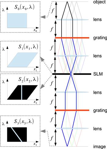
Figure 1. Proposed setup (right), and illustration of the spectral selection done at the output of the SLM and on the detector, in case the SLM only opens a slit (left). f is the focal length of the lenses. The spectral density at the source, just before and after the SLM and at the detector are represented by S0, S1, S2, and S3, respectively.
Download figure:
Standard image High-resolution image2.2. Geometrical optics analysis
In this section a basic analysis of the system is used to obtain an efficient reconstruction algorithm. It is shown that the system acts as a programmable, spatially dependent, spectral filter for which spatial resolution is independent of spectral resolution and for which there is no wavelength dependent shift of the image at the detector. The analysis of this system closely follows that of Gehm et al [9] which models the propagation of the spectral density through the system. The intensity, In, at the nth plane of propagation is given in terms of the spectral density, Sn, as

where xn and yn are perpendicular to the optical axis of propagation and λ is the wavelength. Using geometrical optics propagation, the spectral density of the dispersed image at the SLM, S1, is given by

where S0 is the spectral density at the source, and the central wavelength,  , is the wavelength of light which follows the optical axis of the system. The dispersion of the system (along the x direction) is given by
  where f is the focal length of the lenses, d is the grating periodicity, and
  is the angle at which the central wavelength is diffracted from the grating [10]. The spectral density of the diffracted image after a narrow slice has been selected, S2, is given by

where  is the transmission function corresponding to the SLM. The second grating reverses the spectral shift applied by the first thus giving S3, the spectral density at the detector:

For a simple spectralcunction is given by a rectangular function of width  centred at xm.

Applying this transmission function to the spectral density at the detector gives

The intensity at the detector is determined by integrating the spectral density with respect to wavelength.
where the bounds of integration are determined by the width and position of the rectangular function used as the transmission function and  is the spectral response function of the detector.

Applying  and
and  as the end points of the integral in equation (7) gives the final intensity
  which, assuminsg linearity of the integrand within the bounds of integration, has a spectral resolution
  and is given by

This equation can be slightly rearranged to give

from which the key features of the dual disperser setup can be highlighted.
First, the recorded image  for a given slit position xm on the SLM gives a direct access to a 2D subset of the hyperspectral cube that corresponds to a slanted cut inside the cube along the
  direction (figure 2). The dual disperser acts as a narrow band spectral filter with a linear gradient in wavelength along x3 and the position of the slits on the SLM determines the offset of this gradient.

Figure 2. Illustration of the dual disperser imaging process, in the case when a single slit of the DMD is opened. The slit defines a series of spectral filters that are applied on different spatial areas of the imaged object (top). The final image corresponds to a slanted slice of the original object hyperspectral cube (middle), and there is no wavelength dependent spatial shift on the recorded image (colocation property, bottom).
Download figure:
Standard image High-resolution imageSecond, all the spectral components of the hyperspectral cube sharing the same x and y coordinates are colocated at the same position on the image: a point  of the hyperspectral cube can only affect the intensity at the image position
  . In other words, there is no wavelength dependent spatial shift on the image: the position at which we retrieve an element from the hyperspectral cube on the image does not depend on its wavelength coordinate in the cube.
This implies that there is no need for a complicated reconstruction algorithm to recover the spatial coordinates of points in the hyperspectral cube. Using a simple slit pattern, the whole hyperspectral cube can be readily retrieved by scanning the slit across the SLM and recording the images corresponding to each slit position.
It is also obvious from equation (10) that the spatial resolution of the system does not depend on the parameters which determine spectral resolution (i.e. slit width, grating periodicity, and focal length). The spectral resolution is given by the difference in wavelength corresponding to two neighbouring slit positions at any single point on the detector,  . The dependence of the spectral resolution on slit width and dispersion is the same as that of a conventional spectrometer.
2.3. Gaussian optics modelling
Although, thus far, a finite numerical aperture has not been accounted for in this system, that is the primary limiting factor in terms of spatial and spectral resolutions. It is also important to evaluate the effect of diffraction from the source and SLM. In order to illustrate the scanning method described in the previous section, a simulation was run to mimic the dual disperser system and test the reconstruction method. The model used for this simulation is chosen because it is well established in the field of pulse shaping to describe the effect of an SLM inside a 4-f line [10]. This model, relying on Gaussian optics propagation is fairly fast and naturally reproduces the effect of diffraction and limited numerical aperture. It also reproduces the geometrical distortion introduced by a grating. The propagation of the electric field through a lens of focal length f, as illustrated in figure 3, is given by [10, 11]:

where  and
and  are respectively the electric fields at the image and object planes (both separated from the lens by a distance f) and
  is the central wavelength of the field. The limited numerical aperture of the lens is taken into account by limiting the Fourier transform integral to components that fits within the lens diameter Dl[11]. Similarly, the field immediately after the diffraction by a grating, as illustrated in figure 4, is given by [10, 12, 13]

where d is the grating period and Ei and Ed are the incident and diffracted fields, respectively, and are located at the grating on a plane perpendicular to the direction of propagation of the central wavelength respectively before and after diffraction.  and
and  are the angles of diffraction and incidence corresponding to the central wavelength, respectively, and kC is the wavenumber associated with the central wavelength
  .
.
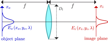
Figure 3. Propagation of the electric field in the Gaussian optics approximation from object to image plane for a lens of focal length f and diameter Dl.
Download figure:
Standard image High-resolution image
Figure 4. Effect of a diffraction grating on the electric field in the Gaussian optics approximation.
Download figure:
Standard image High-resolution imageUsing equations (11) and (12) one can propagate the initial field to the SLM plane, and using the same equations propagate the filtered field from the SLM to the detector plane. It should be noted that if we leave aside the limited numerical aperture by the lenses, the main difference with the analysis done in the previous section is the presence of the scaling factor β that magnifies the image formed at the SLM without affecting the dispersion. The inverse magnification occurs on the way to the detector. Accounting for this in the analysis of the previous section only changes the position dependence of the measured wavelength. Thus, the measured intensity for a given slit position in the disperser in the limit of infinite numerical aperture for the whole setup is

When accounting for the limited numerical aperture of the lenses, the solution cannot be written as simply as the above equation, as it contains many integral terms. However, the core linear dependence in the equation (13) remains valid as the main effect of the limited numerical aperture is to reduce the spatial and spectral resolution of the reconstructed image, exactly like in an imaging spectrometer.
2.4. Simulation
By applying equations (11) and (12) in the right order, propagation through the dual disperser was simulated, using the object image shown in figure 5. An arbitrary central wavelength of  was used for the simulation. The initial object cube contained 31 spectral channels ranging from
  to
to  . The focal length of the lenses, periodicity of the gratings and width of the slit were 40 cm,
  and
and  respectively. The lens diameter was 1 cm. Images were retrieved for 41 different slit positions which resulted in the retrieval of 41 spectral channels ranging from
  to
to  . Spectral images for channels centred at
  ,
,  , and
, and  of the initial object cube are shown figures 6(a)–(c), and the corresponding retrieved object cube channels are shown figures 6(e)–(g). The initial object cube is defined by 31 spectral planes, while the scanning allows to retrieve 41 retrieved spectral planes: the retrieved cube is hence spectrally not sampled exactly as the initial cube, and the figure compares three close channels. The unfiltered initial and reconstructed images are also shown respectively on figures 6(d) and (h). The model takes into account the limited numerical aperture of the lenses: the imager is not collecting all the light out of the initial cube, which introduces, like in a real device, some vigneting and loss of spatial resolution. This simulation demonstrates the effectiveness of the model described in section 2 in terms of reconstructing a hyperspectral image, as well as getting an unfiltered image of the object.

Figure 5. A schematic representation of the object cube used for the simulation, defined by a light source and an c-shaped aperture. The illumination is composed of 31 different wavelengths, each corresponding to a Gaussian spatial profile with a different width and location along the y-axis.
Download figure:
Standard image High-resolution image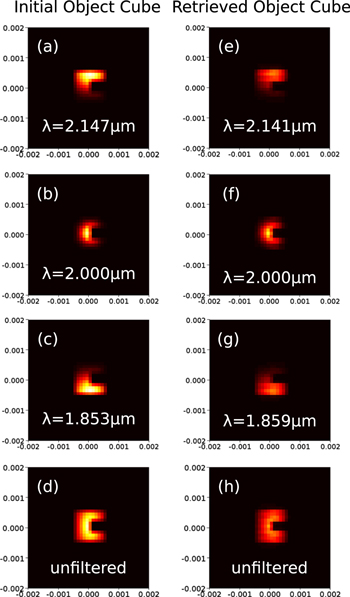
Figure 6. (a), (b), (c) individual wavelength images of the hyperspectral object cube defined in figures 5; (e), (f), (g) Retrieved individual wavelength images; (d) unfiltered initial image; (h) unfiltered retrieved image.
Download figure:
Standard image High-resolution imageThe scheme presented here relies on a scanning process: the slit position on the SLM needs to be scanned to retrieved the whole hyperspectral cube. The scanning can be extremely fast (well beyond video rate) by using modern SLM like digital micromirror devices (DMD) or liquid crystal on silicon found in most projectors. But contrary to traditional scanning hyperspectral imagers, we can easily access the unfiltered image in a single shot, and also set the trade-off between number of retrieved spectral channels and acquisition time while keeping the maximal spatial resolution available. Additionally, near snapshot acquisition of the hyperspectral cube can be achieved under certain conditions by using more subtle patterns than a single slit, as described in the next section.
3. Near snapshot partitioning
Here we exploit both the easy access to a full-resolution unfiltered image and the colocation of all the spectral components on the final image to propose a simple way to achieve near snapshot acquisition of hyperspectral data.
The starting point is the assumption that there exist in the hyperspectral cube spatial regions that are 'spectrally homogeneous', i.e. for which every pixel (x, y) has the same spectrum:  , where
  . This is a reasonable sparsity assumption that holds in numerous real scenes, where the spectral content is strongly spatially correlated. One straightforward way to identify these regions is to look for contiguous regions of iso-intensity on the unfiltered image obtained with all the DMD pixels opened: assuming such regions are spectrally homogeneous and exploiting equation (13), the spatial coordinates in the region can be used to encode different spectral channels.
A canonical example of a homogeneous region is presented on figure 7 (top): it is one horizontal segment of pixels ![$[A,B]$](https://content.cld.iop.org/journals/2040-8986/17/8/085607/revision1/joptaa0068ieqn34.gif) along the x direction, xA and xB denoting its starting and ending x coordinates. For a simple slit pattern programmed on the SLM at the position xm, the intensity
along the x direction, xA and xB denoting its starting and ending x coordinates. For a simple slit pattern programmed on the SLM at the position xm, the intensity  on the final image along this segment corresponds to the spectral density
  :
:

with λ in the range ![$\left[{\lambda }_{A},{\lambda }_{B}\right]$](https://content.cld.iop.org/journals/2040-8986/17/8/085607/revision1/joptaa0068ieqn37.gif) . The width
. The width  of the homogeneous region directly determines the bandwidth
  over which the spectral density is recovered. Moreover, for a given position of the homogeneous region, the position xm of the slit on the SLM can be used to set the central wavelength of the recovered range. If the homogeneous region is wide enough, its whole spectral density can be retrieved in a single acquisition—the 'whole spectrum' being defined by the parameters α and β, and its resolution being defined by the CCD resolution.

Figure 7. Snapshot partitioning: in spectrally homogeneous regions, the spatial coordinates in the final image can be used to encode all the spectral channel by a simple choice of multi-slit pattern to apply on the SLM. Top: if the region is wide enough, its whole spectrum can be recovered by opening just one slit of the DMD. Bottom: if the region is not wide enough, its vertical span can be exploited to recover the whole spectrum, by positioning slits so as to recover portions of the spectrum which can be concatenated afterwards.
Download figure:
Standard image High-resolution imageThe region width limits the observable spectral range, but its height can be exploited to extend this range. Figure 7 (bottom) shows a rectangular region spanning in both x and y directions: in that case, the region can be subdivided along the y direction in several horizontal segments ![$[{A}_{i},{B}_{i}]$](https://content.cld.iop.org/journals/2040-8986/17/8/085607/revision1/joptaa0068ieqn40.gif) with the same starting and ending x coordinates
with the same starting and ending x coordinates ![$[{x}_{A},{x}_{B}]$](https://content.cld.iop.org/journals/2040-8986/17/8/085607/revision1/joptaa0068ieqn41.gif) . A multi-slit pattern can be applied on the SLM in order to match each segment
. A multi-slit pattern can be applied on the SLM in order to match each segment ![$[{A}_{i},{B}_{i}]$](https://content.cld.iop.org/journals/2040-8986/17/8/085607/revision1/joptaa0068ieqn42.gif) with a given slit position xmi, so that portions of the spectral density can be retrieved. This principle can be straightforwardly applied to homogeneous regions of arbitrary shape: their spectrum can be recovered by dividing them into i slices of width
with a given slit position xmi, so that portions of the spectral density can be retrieved. This principle can be straightforwardly applied to homogeneous regions of arbitrary shape: their spectrum can be recovered by dividing them into i slices of width  and height
  , for each of which a slit is selected on the SLM. From each slice a spectral bandwidth
  can be recovered, the maximum recoverable spectrum being defined by the accumulated width of the slices.
This principle can easily be generalized to analyse in a single acquisition the spectrum of several regions detected in the unfiltered images. The relative positions and shapes of the detected regions must be considered: any two regions which are completely separated along the y-axis can be analysed in the manner described above, as slits used to measure the spectral content in any part of one region have no effect on the measurement of any part of the other region. For regions which overlap along the y-axis, the solution depends on the geometry of the two regions and on the extent to which they overlap. Simple partitioning strategies illustrated in figure 8 can be straightforwardly defined.
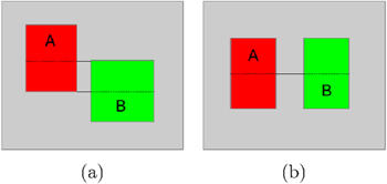
Figure 8. (a): the spectrum of two regions partially overlapping along the y axis can be measured by acquiring the spectral information from sub-regions A and B. (b): the case where two regions that fully overlap along the y axis can be addressed by selecting non-overlapping sub-partitions A and B.
Download figure:
Standard image High-resolution imageSo by taking an unfiltered initial image, partitioning it in homogeneous regions of uniform intensity and assuming they have the same spectral content, simple geometric reasoning can be exploited to automate the extraction of their spectral content. One key point is that the simplicity of equation (14) results in a straightforward relation between the slit patterns on the SLM and the position of each spectral component on the final image. Various multi-slit patterns can be used for a given region and a given spectral density, and if the region is wider than the strict minimum to retrieve its spectral density, one can multiplex several measurements of the spectral density: this could for example be exploited to assess the validity of the region spectral homogeneity assumption.
4. Preliminary results
4.1. Setup and calibration
To demonstrate the models and techniques described in sections 2 and 3 a prototype has been set up (figures 9 and 10). The observed object consists of a light source placed behind a lithographic mask. The mask is followed by a  focal-length lens, a
  periodicity grating set for a deviation angle of around
  , a
, a  -lens, and a DLP lightcrafter DMD. The DMD was set up to reflect the first diffraction order straight back along its incident path, thus reusing all of the optics of the first half of the dual disperser as the second half. A beam splitter is placed between the source and the first lens in order to direct the final image onto a camera. The camera is a standard CMOS camera (monochromatic IDS uEYE).
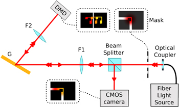
Figure 9. Schematic view of the experimental setup used for verification of models and techniques proposed in sections 2 and 3. A DMD is used as the SLM and reflects the selected light straight back along the incident path, thus reusing grating and lenses. A beamsplitter is used to redirect the final image onto the CMOS camera.
Download figure:
Standard image High-resolution image
Figure 10. View of the actual experimental setup.
Download figure:
Standard image High-resolution imageA lithography mask serves as a test pattern with sharp spatial features. To test our setup with different spectral contents, two collimated beams were alternatively used to illuminate the mask: a Superlum BroadLighter S840, providing an incoherent  -wide spectrum centred at
  or a Superlum BroadSweeper 840 providing coherent and narrow spectrum (down to
  ), tunable between
  and
and  . This latter source can also quickly sweep to generate dual wavelength spectra or broad square spectra. The resulting test object resembles the one of figure 5, where an illuminating beam is spatially filtered by an aperture.
A simple linear calibration of the dispersion on the SLM was carried out by recording CMOS images as a function of the slit position on the SLM for several monochromatic spectra between  and
and  . This calibration gives
  with
with  ,
,  and
and  , and where x3 is the x-position on the CMOS camera and xm the slit position on the DMD as in equation (13), all dimensions being in
  . The spectra measured on each point of the CMOS image with our setup were compared with independent measurements made on the light sources using an optical spectrum analyser (OSA Ando AQ6315-A).
4.2. Scanning slit
To assess the validity of the system model and calibration, first measurements were made with the scanning technique described in section 2. Two typical results are shown in figures 11 and 12, respectively for a dual wavelength spectral content and for a broad spectrum. In both figures, sub-figure (a) show the unfiltered image that integrates the whole spectral content image (all pixels of the DMD being opened), and the region of interest (ROI) in which the spectrum is recovered. Sub-figures (b) show the recovered  slice of the cube corresponding to the ROI, and sub-figures (c) show the averaged spectrum retrieved over the ROI, compared to the OSA measurements.

Figure 11. Hyperspectral measurement obtained with a moving slit scheme, for a dual wavelength illumination of the mask. The analysed ROI is denoted by a green rectangle in (a), and figure (b) shows the associated  slice of the cube (the green arrow helps to match the x coordinates in both images). Figure (c) compares the average retrieved spectrum of the ROI (in orange) with the spectrum independently retrieved by the OSA (in blue).
Download figure:
Standard image High-resolution image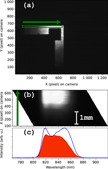
Figure 12. Hyperspectral measurement obtained with a moving slit scheme, for a nearly homogeneous  wide spectrum centred at
  illumination of the mask (see caption of figure 11).
Download figure:
Standard image High-resolution imageIn both figures, one can see that within the ROI, the spectral and spatial variations of the spectral density are not coupled: the spectral density can be represented by a product of one spatial and one spectral functions. This is coherent with our test hyperspectral cube that can be separated in a spectral function (the spectral content of the tunable laser or superluminescent diode) and a spatial one (the Gaussian-like spatial profile of the illuminating beam, clipped by our lithography mask). One can also observe (in subfigure (b)) that the accessible spectral range shifts linearly with the x-position on the CMOS camera, in agreement with equation (13).
In figure 11(c), one can see a good agreement between the reported wavelength by our prototype and the OSA, but also notice a small difference in the relative intensities of the two spectral peaks.
Another noticeable difference appears in figure 12(c), where a significant intensity mismatch appears for wavelengths above  nm. This is due to the lack of spectral efficiency calibration in our setup (contrary to the OSA, which is properly calibrated). This is compatible with the spectral efficiency of the CMOS camera used in the setup, that drops by a factor of 2 from
  to
to  .
.
To better illustrate the fidelity of the retrieved spectrum, we measured it at the centre of the ROI defined in figure 12 for different sources and compared it with independent OSA measurements of the source spectrum. Results are presented in figure 13, with several 5 nm wide square spectra, and with the super-luminescent source in high and low power mode. These measurements confirm that apart from a the lack of intensity calibration (visible for wavelengths above  nm), the prototype reproduces the spectral content of the test object. This validates the basic scanning method proposed in section 2, and this especially shows that a straightforward coarse calibration of the system allows to recover precise spectral information.

Figure 13. Comparison between the spectrum retrieved at the centre of the ROI defined in figure 12 (orange) and measured by the OSA (blue) for various source settings: (a), (b):  wide square spectra starting at different wavelength ranging from 820 to
  ; (c), (d): super-luminescent broad source for two different power settings.
Download figure:
Standard image High-resolution image4.3. Near snapshot partitioning
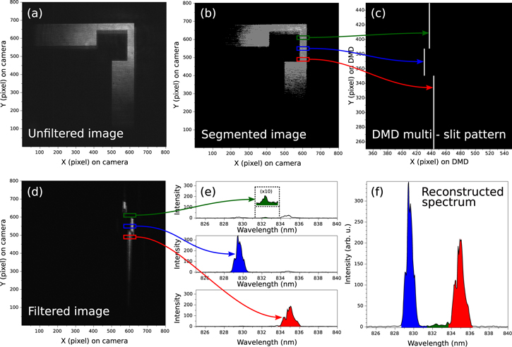
A second set of measurements illustrates the near snapshot technique described in section 3 to retrieve in just two acquisitions the full spectrum of a dual wavelength source (830 and  nm) in a ROI detected in the unfiltered image. Figure 14 illustrates the step of the process: (a) shows the unfiltered image (first acquisition), which is coarsely segmented into regions of homogeneous intensities (b). The selected ROI is the narrow vertical portion of the lithographic mask. This ROI is not wide enough to allow the recovery of a large spectrum by opening only a single slit in the DMD: we are in a case similar to the one of figure 7 (bottom). Hence various slit positions are required to recover its spectrum: three areas are selected in the ROI (green, blue and red rectangles of (b)), and a slit position is defined in the DMD for each of these areas, so as to independently recover a part of their spectrum over three intervals
 ![$\left[{\lambda }_{A}^{i},{\lambda }_{B}^{i}\right]$](https://content.cld.iop.org/journals/2040-8986/17/8/085607/revision1/joptaa0068ieqn73.gif) , i denoting the area index (the width of the areas defines the width of the recoverable spectral interval, the position of the slit defines the central wavelength of this interval; see section 3). The slit arrangement is shown in (c), and the resulting filtered image captured by the CCD is shown in (d) (second acquisition). The spectrum recovered for each area is shown in (e), and the whole spectrum of the ROI is shown in (d): it is coherent with the illuminating source spectrum. An issue here is the precise intensity ratio between the
, i denoting the area index (the width of the areas defines the width of the recoverable spectral interval, the position of the slit defines the central wavelength of this interval; see section 3). The slit arrangement is shown in (c), and the resulting filtered image captured by the CCD is shown in (d) (second acquisition). The spectrum recovered for each area is shown in (e), and the whole spectrum of the ROI is shown in (d): it is coherent with the illuminating source spectrum. An issue here is the precise intensity ratio between the  and
and  peaks, due to the slight intensity inhomogeneity within the ROI: intensity in the red area is slightly lower than in the two other areas, which leads to an underestimation of the spectrum part measured in the red area.
Figure 14. The full spectrum of a ROI is precisely recovered in only two image acquisitions (see text for details).
Download figure:
Standard image High-resolution image
5. Conclusion
The concept of a simple adaptive method of hyperspectral imaging with the possibility for near snapshot imaging of spatially sparse scenes has been illustrated by modelling, computer simulations, and validated with preliminary experiments. The proposed method requires negligible reconstruction time and allows for applications with different spatial and spectral resolution requirements, as well as easy access to a full spectrum image without requiring any modification of the system setup.
More precise measurements would require a more thorough spectral and intensity calibration. It should however be noted that thanks to the colocation property not only such a calibration is relatively straightforward to apply compared to existing techniques [7], but also it is not required to obtain reasonably accurate results, as shown by our preliminary results.
The proposed system and its model open further possibilities. For instance, it is possible to use a scanning technique to take real-time, video-rate images of any single wavelength. This would rely on a slit scanning technique similar to that which is described in section 2.2, but measuring only one slice of the image for each slit position rather than the entire image. By synchronizing the rolling shutter of a CMOS with the scanning slit, one would indeed recover a single wavelength image, the wavelength of each frame being defined by the delay between the two devices.
For simple scenes where the spectrum is strongly spatially correlated, automated, real-time, near-snapshot analysis may be achieved with the presented region partitioning approach. The associated algorithms can easily be extended, e.g. to retrieve a set of given spectral channels on homogeneous regions instead of their full spectrum. But the spectral analysis of complex scenes may require more sophisticated techniques: the system allows the development of compressed sensing schemes, that would dynamically drive the SLM according to the perceived scene and the spectral information required by the considered task.
Acknowledgments
This work was partially funded through a resourcing action of the LAAS CNRS Carnot Institute, namely, HyperHolo project (Hyperspectral holographic imager with high performance). This work was also granted access to the HPC resources of CALMIP supercomputing center under the allocation 2014-[P1419].