
Abstract
This work introduces a theoretical framework to describe the dynamics of reacting multi-species fluid systems in-and-out of equilibrium. Our starting point is the system of generalised Langevin equations which describes the evolution of the positions and momenta of the constituent particles. One particular difficulty that this system of generalised Langevin equations exhibits is the presence of a history-dependent (i.e. non-Markovian) term, which in turn makes the system's dynamics dependent on its own past history. With the appropriate definitions of the local number density and momentum fields, we are able to derive a non-Markovian Navier–Stokes-like system of equations constituting a generalisation of the Dean–Kawasaki model. These equations, however, still depend on the full set of particles phase-space coordinates. To remove this dependence on the microscopic level without washing out the fluctuation effects characteristic of a mesoscopic description, we need to carefully ensemble-average our generalised Dean–Kawasaki equations. The outcome of such a treatment is a set of non-Markovian fluctuating hydrodynamic equations governing the time evolution of the mesoscopic density and momentum fields. Moreover, with the introduction of an energy functional which recovers the one used in classical density-functional theory and its dynamic extension (DDFT) under the local-equilibrium approximation, we derive a novel non-Markovian fluctuating DDFT (FDDFT) for reacting multi-species fluid systems. With the aim of reducing the fluctuating dynamics to a single equation for the density field, in the spirit of classical DDFT, we make use of a deconvolution operator which makes it possible to obtain the overdamped version of the non-Markovian FDDFT. A finite-volume discretization of the derived non-Markovian FDDFT is then proposed. With this, we validate our theoretical framework in-and-out-of-equilibrium by comparing results against atomistic simulations. Finally, we illustrate the influence of non-Markovian effects on the dynamics of non-linear chemically reacting fluid systems with a detailed study of memory-driven Turing patterns.
Export citation and abstract BibTeX RIS

Original content from this work may be used under the terms of the Creative Commons Attribution 4.0 licence. Any further distribution of this work must maintain attribution to the author(s) and the title of the work, journal citation and DOI.
1. Introduction
Many applications, from chemistry to biology and engineering, exploit complex fluids consisting of colloidal particles. A number of challenging issues in applications requires chemically reacting particles while colloidal chemistry is often the preferred path for particulate systems and formulated products. Examples range from the design of micro-/nanofluidic devices [1], lab-on-chip applications [2] and analysis of chemical reactors [3] to biological macromolecules in solutions [4], dispersion of carbon nanotubes in solvents [5] and preparation–formulation of organic nanoparticles [6].
Physical properties at the nanoscale may be investigated in a 'brute-force' manner by solving the Newton's equations of motion for each individual particle, i.e. by means of molecular dynamics or Monte Carlo simulations. However, many interesting dynamical events, such as protein folding [7, 8] and phase nucleation [9, 10], occur at time- and lengthscales several orders of magnitude larger than those accessible by atomistic simulations [11]. Due also to the prohibitively high computational cost associated with such simulations, coarse-graining remains a highly relevant instrument in the study of reacting systems. Precursory model reduction techniques go back to the phenomenological description of pollen particles in water by Brown [12]. However, it was not until the work of Langevin [13] that a low-dimensional (stochastic) model for such phenomena was formulated. Since then, several reduced models have been proposed [14–26]. A standard way to coarse-grain a system is by using projection-operator techniques to decouple the relevant and the non-relevant degrees of freedom in the system [16, 20, 25, 27]. This leads to a system of stochastic generalized Langevin equations (GLEs) for the time evolution of the resolved variables (relevant degrees of freedom). The effects of the unresolved variables (the irrelevant degrees of freedom) are included as the noisy part of the GLEs. Such GLEs typically have non-Markovian terms involving time convolutions which carry information about the history of the dynamical system at hand. Most existing studies focus on the so-called Markovian limit of the full GLEs where the memory effects are ignored [28, 29]. Importantly, the Markovian approximation can be inaccurate when the system does not have a clear scale separation between the resolved and the unresolved variables. It is worth underlying that, in general, GLEs are used to describe the stochastic time-evolution of a set of observables of interest of a dynamical system. These observables can be either some particle coordinates (microscopic observables) or continuum field variables (macroscopic observables). In this work, GLEs are used to obtain the time evolution of some particle coordinates of interest (or resolved particles). It follows that this Langevin approach still gives a description of the system at particle-level, and thus it is essentially equivalent in computational complexity to atomistic simulations.
A continuum/mean-field framework capable of describing small-scale systems is offered by density-functional theory (DFT) or its dynamical counterparts known as dynamical DFT (DDFT), and fluctuating hydrodynamics (FH). Unlike the atomistic GLEs, both DDFT and FH operate with local averaged densities and are thus computationally tractable. DDFT is usually obtained by deriving the Fokker–Planck equation governing the evolution of the system probability density function, which is then averaged over all but one degrees of freedom [22, 30–32]. Recently, several extensions of DDFT were proposed for multi-component systems [30] to include hydrodynamic interactions [31–33] and effects of particle orientability [34]. On the other hand, FH for simple liquids was initially stipulated by Landau et al from empirical arguments [35]. The connection between FH and the density-functional framework for small-scale systems was later highlighted in the works of Kawasaki and Dean (DK) [28, 36] (with Dean's equation being the overdamped counterpart of Kawasaki's). In the DK approach, a heuristic energy functional accounting for small-scale features was introduced. Recently, a rigorous and systematic derivation of FH and fluctuating DDFT (FDDFT) for the general case of arbitrarily shaped thermalized particles was offered by Durán-Olivencia et al [34].
It should be emphasised, however, that the DK model describes the evolution of instantaneous microscopic fields, thus containing the same physical information as the original set of GLEs, and hence leaves the equations computationally intractable and at the same time disconnected from the original Landau et al theory. Even more importantly, this disconnection has often led to the misconception that the DK model describes the evolution of macroscopic observables. The formalisation of the connection between DK and FH to enable the description of the evolution of observable fields and remove the dependence on the microscopic GLEs has lately received a great deal of attention. Indeed, recent efforts have achieved the desired formal connection under the local-equilibrium approximation [29, 37]. Finally, applications of FH to multi-component reacting systems have been studied in many works, e.g. references [38–40].
Thus far, the inclusion of fluctuations in the DDFT framework has posed many questions [41]. For instance, in some studies such as the work by Elder et al [42], an additional noise term was artificially included, but the physical meaning of this term remains questionable. At the same time, the derivation of the Fokker–Planck equation, the first step in the derivation of DDFT, requires that we already averaged out the noise. The recent effort by Durán-Olivencia et al [29] showed that DDFT can be understood as the most-likely realisation of FDDFT, thus providing closure to a long standing debate in the density-functional theory community about the inclusion of fluctuations establishing also rigorously the connection between FDDFT and FH from first principles.
In the present work we start with microscopic GLEs of reacting systems to derive the corresponding FH equations. The underlying GLEs allow us to obtain the proper noise correlations in FH, as well as include memory effects. We derive the non-Markovian FH governing the time evolution of the one-body density and momentum fields in systems of several reacting species. Adopting a density-functional formulation, we transform the FH equation to an equivalent FDDFT equation. In the appropriate overdamped limit, the latter reduces to a single equation for the time-dependent one-body density field.
In general, numerically solving the non-Markovian FH is quite challenging due to the memory term and the time-correlated noise. For a memory term in the form of decaying exponential series, the computational issues are overcome by introducing an additional field, whose time evolution accounts for both the memory term and noise time correlations. Such an approach will be denoted as 'extended field dynamics'. The resulting non-Markovian DDFT equations are then solved numerically using a finite-volume approach. Our numerical scheme is exemplified with several applications to multi-component reacting systems leading to the emergence of stochastic Turing patterns [43–51].
In section 2 we introduce the GLEs for an isothermal multi-component system of particles, which provide the starting point for our derivation. Section 3 deals with the inclusion of microscopic density and momentum fields, and the derivation of the FH equations for a multi-species reacting system. A non-trivial deconvolution operator has to be defined to take the overdamped limit of the previously derived FH. This leads to the formulation of a non-Markovian overdamped FDDFT equation for the density field in section 4. The computational challenges due to both the memory term and the correlated noise are overcome by introducing an extended-field variable dynamics framework in section 5. The finite-volume method is then adopted for the spatiotemporal discretization of the extended variable dynamics in section 6. Section 7 reports several computational experiments including a comparison between molecular dynamics simulations and FH that validates our main theoretical results, and a dedicated study of memory-driven Turing patterns. Conclusions and outlook for possible future work are offered in section 8.
In figure 1, we show a flowchart summarizing the main equations in this work and their connections to previous formulations. Moreover, for the sake of clarity, we include in table 1 a summary of the abbreviations used in the text and their definition.

Figure 1. Flowchart showing the approach followed to obtain the non-Markovian FDDFT and its overdamped approximation. The interconnections to previous formulations are also included. Arrows denote the relations among the different approaches. Thin boxes/arrows: previous approaches. Thick boxes: main results of this work. Text and equations on arrows provide a brief explanation of the main approximations or manipulations.
Download figure:
Standard image High-resolution imageTable 1. List of abbreviations and corresponding definitions adopted in the manuscript.
| Abbreviations | Definitions |
|---|---|
| GLE | Generalized Langevin equation |
| DFT | Density functional theory |
| DDFT | Dynamical DFT |
| FDDFT | Fluctuating DDFT |
| FH | Fluctuating hydrodynamics |
2. GLEs
Consider an isolated system containing a total of Ntot,s
(t) particles at time t, with s = 1, ..., K denoting the different coexisting species. The phase-space coordinates of a given species s are noted as zs
= {rs
, ps
}, with  and
and  being the particle positions and momenta, respectively. In many cases, such as colloids in suspension, one is interested in the dynamical evolution of only the first Ns
of the original Ntot,s
particles belonging to the species s. The coordinates of the particles of interest are also known as resolved variables, while the remaining ones are denoted as unresolved variables or thermal bath. Using time-scale separation (or weak coupling) between resolved and unresolved variables, the resolved ones can be shown to obey the following GLE [16, 20, 25, 56]:
being the particle positions and momenta, respectively. In many cases, such as colloids in suspension, one is interested in the dynamical evolution of only the first Ns
of the original Ntot,s
particles belonging to the species s. The coordinates of the particles of interest are also known as resolved variables, while the remaining ones are denoted as unresolved variables or thermal bath. Using time-scale separation (or weak coupling) between resolved and unresolved variables, the resolved ones can be shown to obey the following GLE [16, 20, 25, 56]:
where  is the effective force experienced by each particle, with U(
r
i,s
) being the potential of mean force in the form:
is the effective force experienced by each particle, with U(
r
i,s
) being the potential of mean force in the form:

where Vα is the two-body interacting potential acting between particles of the species s and α, and Uext is the external potential acting on the system. It is worth highlighting that the underlying assumption in equation (2) is that the inter-particle interactions are governed by one- and two-body interactions. While this assumption allows us to significantly simplify the derivation in what follows, it also poses some limitations. In fact, the energy functional that we derive is only able to account for the two-body correlations. For applications requiring higher-order interactions, the assumption could be relaxed, and our derivation could be easily extended in order to account for any N-body interactions. Should this be the case, the structure of the equations derived hereinafter [specifically equation (26)] would lead to the exact first equation of the YBG hierarchy, which involves all N-body densities, and hence correlations.
The second term on the right-hand side of equation (1) is widely known as the damping force, representing the deterministic drag coming out from the random collisions of the target particles with the surrounding bath particles. Such a drag force involves a memory-kernel tensor θ s (t) which makes the force dependent on the entire history of the particle dynamics [25, 26, 52–55]. It is worth noticing that if the thermal bath is characterized by multiple timescales, the dynamical effects of the bath particles of the original system may not be fully embedded in the memory kernel θ s (t) of equation (1). But these applications are beyond the scope of this work.
The stochastic term R i,s (t) in equation (1) accounts for the volatility which the just mentioned collisions with the bath induces on the particle's acceleration. This emerges as a Gaussian distribution with zero mean and a correlation function satisfying the fluctuation dissipation theorem:

where kB is Boltzmann's constant, T is the absolute temperature imposed by the system of bath particles and the brackets ⟨⋅⟩ denote the ensemble average over multiple realizations of the noise, i.e. ⟨A⟩ = ∫ ρ(z)A(z) dz, with ρ(z) being the probability density function defined in the phase space of the original system. Despite being derived for equilibrium conditions, in this work equation (3) is also applied to systems in local-equilibrium. This extension is rigorously valid if the thermal bath is assumed to relax instantly toward local-equilibrium conditions. For the sake of clarity, we need to highlight that all particles of the same species, say s, have the same mass and memory kernel and interact only via the pairwise potential Vs , as specified in equation (2).
Some systems are characterized by a time-scale separation between resolved and unresolved particle dynamics, due for instance to the much higher inertia of the first compared to the latter particles. In these cases, the memory kernel tensor in equation (1) can be approximated as
θ
s
(t) = 2
θ
s,0
δ(t), where δ(t) is a Dirac's delta function and
θ
s,0 is a constant. This approximation allows one to obtain a memory-less (or Markovian) formulation, with a much simpler structure. In fact, in the Markovian limit the memory term in equation (1) loses its convolution structure, i.e.  , while the stochastic term becomes delta-correlated in time, i.e. ⟨
R
i,s
(t)
R
i,s
(t')⟩ = ms
kB
T
θ
s,0
δ(t − t') [26]. However, when no clear scale separation between colloidal and bath particles is present, the Markovian hypothesis is not applicable and one needs to seek a way of approximating the memory kernel to numerically track the dynamics [21, 23, 25, 56].
, while the stochastic term becomes delta-correlated in time, i.e. ⟨
R
i,s
(t)
R
i,s
(t')⟩ = ms
kB
T
θ
s,0
δ(t − t') [26]. However, when no clear scale separation between colloidal and bath particles is present, the Markovian hypothesis is not applicable and one needs to seek a way of approximating the memory kernel to numerically track the dynamics [21, 23, 25, 56].
In a recent study on the parameterization of GLEs, Lei et al used a data-driven approach to approximate the memory kernel [56]. Following this study, one could consider atomistic observations of a system at equilibrium, then right-multiply equation (1) by the initial momentum p i (0) and, finally, take the ensemble average with respect to the equilibrium distribution function, obtaining the following equation:

where we have defined the matrices  and
and  and made use of the orthogonality between the stochastic term and the particle momentum, i.e. ⟨
R
i,s
(t) ⋅
p
i,s
(0)T
⟩ = 0 [25]. Taking the Laplace transform
1
of equation (4), we get
and made use of the orthogonality between the stochastic term and the particle momentum, i.e. ⟨
R
i,s
(t) ⋅
p
i,s
(0)T
⟩ = 0 [25]. Taking the Laplace transform
1
of equation (4), we get

where  ,
,  and
and  denote the Laplace transforms of
h
i,s
(t),
g
i,s
(t) and
θ
s
(t), respectively. Assuming that the memory kernel θ(t) is isotropic and represented in the form of decaying exponential series,
denote the Laplace transforms of
h
i,s
(t),
g
i,s
(t) and
θ
s
(t), respectively. Assuming that the memory kernel θ(t) is isotropic and represented in the form of decaying exponential series,  , we can express its Laplace transform as:

where I is the identity matrix with dimension 1, 2 or 3 depending on the dimensionality of the system, As,k and Bs,k are real-valued and Bs,k ⩽ 0. In a data-driven approach, if the matrices h i,s (t) and g i,s (t) are computed from historical data, the sets of coefficients {As,1, ..., As,k , ..., As,d } and {Bs,1, ..., Bs,k , ..., Bs,d } can be fitted using equations (5) and (6).
3. Non-Markovian fluctuating hydrodynamics (FH)
The goal of this section is to go from the non-Markovian GLEs to a more hydrodynamic picture of the equations. For this, we introduce the microscopic number and momentum density fields of species s, containing a number of particles Ns (t) evolving in time according to the particle reactions:
where Ns is the number of particles in species s.
To obtain the time-evolution equations governing the dynamics of the microscopic densities just introduced, equation (7) must be differentiated with respect to time, which can be done by applying the discrete Leibniz integral rule:
It is convenient to express the derivative of the discrete upper summation limit in the distribution form,  , where κ indicates the reaction rate. The second term in the right-hand side of equation (8), which in our case will be stochastic in nature, can then be determined empirically [57].
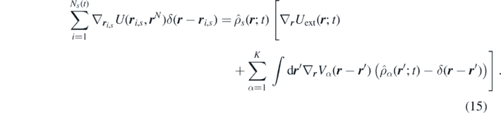
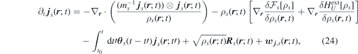
Applying the time derivative defined in equation (8) to the equation (7), and using equation (1), we obtain the time evolution of the number and momentum density fields of each species s:

where  and
and  are the contributions to density and momentum due to chemical reactions, and the local random force
η
s
is:
are the contributions to density and momentum due to chemical reactions, and the local random force
η
s
is:

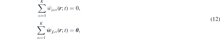
Notice that the terms  and
and  in general allow for reactions between the non-resolved variables and particle sources. However, if reactions can occur between resolved particles only, the conservation of mass and momentum of the total system must also be imposed:
Finally, we can rewrite the noise term without changing its statistical properties (see appendix

where R s denotes the spatial-temporal noise satisfying the fluctuation-dissipation theorem

where kB denotes the Boltzmann constant.
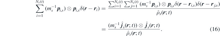
The first and the second terms in the right-hand side of equation (10) can be rewritten now in terms of  and
and  . The second term with the force
F
i,s
, experienced by the particle can be further rewritten as
. The second term with the force
F
i,s
, experienced by the particle can be further rewritten as
The convective flux then becomes [29, 61]
It is worth underlying that, as discussed extensively in references [29, 61], the approach followed to obtain the convective flux in equation (16) is mathematically rigorous only if a physical interpretation of the Dirac delta function is accepted. Specifically, if the phase space is partitioned in cells each containing a single particle, the Dirac delta can be approximated as a Kronecker delta normalized with respect to the volume of the cell. As highlighted in [29], such approximation is strictly valid only for particle systems with a repulsive hard core, which represent by far the most common kind of systems studied in classical particle physics.
Thus, the fluctuating momentum-moment equation reads
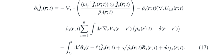
The following definitions of the kinetic, internal and external energy functionals
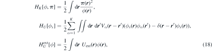
allow us to rewrite equation (17) in terms of the functional derivative of equation (18) as
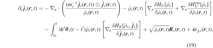
Notice that equation (19) still depends on all particle positions and momenta through the terms  and
and  . Thus, a proper ensemble average is required to obtain a mesoscopic description of the system [29]. With this aim, Durán-Olivencia et al extended the concept of equilibrium canonical distribution, well known from classical statistical mechanical arguments, to local-equilibrium conditions. Local-equilibrium conditions are out-of-equilibrium configurations of the system under which the particles, despite having small deviations from their equilibrium velocities and energies, behave locally as in equilibrium. This approach allows us to take the ensemble average of the system out-of-equilibrium, under a local-equilibrium approximation. To this end, we introduce a probability density function fle(
r
N
,
p
N
; t) for the system in local-equilibrium condition:
. Thus, a proper ensemble average is required to obtain a mesoscopic description of the system [29]. With this aim, Durán-Olivencia et al extended the concept of equilibrium canonical distribution, well known from classical statistical mechanical arguments, to local-equilibrium conditions. Local-equilibrium conditions are out-of-equilibrium configurations of the system under which the particles, despite having small deviations from their equilibrium velocities and energies, behave locally as in equilibrium. This approach allows us to take the ensemble average of the system out-of-equilibrium, under a local-equilibrium approximation. To this end, we introduce a probability density function fle(
r
N
,
p
N
; t) for the system in local-equilibrium condition:

where  is the partition function,
  and
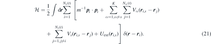
and  is the Hamiltonian given by:
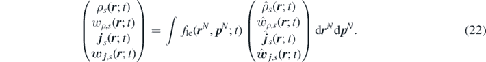
Hence, the ensemble average of density, momenta and reaction sources become fields:
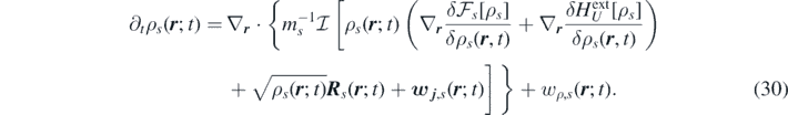
Ensemble averaging equation (19) yields the mesoscopic FDDFT for species s:

where we introduced the free-energy functional, defined as sum of ideal and excess-over-ideal contributions ![${\mathcal{F}}_{s}\left[\rho \right]={\mathcal{F}}_{s}^{\mathrm{i}\mathrm{d}}\left[{\rho }_{s}\right]+{\mathcal{F}}_{s}{\left[{\rho }_{s}\right]}^{\mathrm{e}\mathrm{x}}$](https://content.cld.iop.org/journals/1751-8121/53/44/445007/revision3/aab9e8dieqn22.gif) [29]:
[29]:

with Λ the thermal de Broglie wavelength. The excess part of the free energy is defined through the relation:

where  is the inter-species pair-correlation function. The functional
 ![${\mathcal{F}}_{s}\left[\rho \right]$](https://content.cld.iop.org/journals/1751-8121/53/44/445007/revision3/aab9e8dieqn24.gif) satisfies the relation:
satisfies the relation:

which represents the first equation of the Yvon–Born–Green hierarchy if the averages are taken at equilibrium. For this reason, the functional ![${\mathcal{F}}_{s}\left[\rho \right]$](https://content.cld.iop.org/journals/1751-8121/53/44/445007/revision3/aab9e8dieqn25.gif) can be interpreted as the classical Helmholtz free-energy functional (a more extensive discussion is available in reference [29] and references therein). Notice that in local equilibrium, the term containing the Helmholtz free energy is associated with pressure. In fact, from the Gibbs–Duhem relation (dp = ∑s
ρs
dμs
), and the Euler–Lagrange equation of equilibrium density functional theory (
can be interpreted as the classical Helmholtz free-energy functional (a more extensive discussion is available in reference [29] and references therein). Notice that in local equilibrium, the term containing the Helmholtz free energy is associated with pressure. In fact, from the Gibbs–Duhem relation (dp = ∑s
ρs
dμs
), and the Euler–Lagrange equation of equilibrium density functional theory (![${\mu }_{s}=\delta {\mathcal{F}}_{s}\left[{\rho }_{s}\right]/\delta {\rho }_{s}$](https://content.cld.iop.org/journals/1751-8121/53/44/445007/revision3/aab9e8dieqn26.gif) ) we get:
) we get:

which is consistent with the well-known expressions for one-component systems [29, 59].
The terms wρ,s
and
w
j
,s
represent the average density and momentum reaction rates. The density reaction rate wρ,s
depends on the average number of particle changing species, and thus it can be modeled or directly measured from experiments [see for instance equation (76)]. The momentum reaction rate
w
j
,s
accounts for the average momentum transfer rate between particles during the reaction events. If reactions occur only between resolved particles, i.e. for systems with non-reactive thermal baths, the conservation of mass and momentum of the total system is satisfied, i.e.  and
and  . Moreover, for isotropic reactions, i.e. when the reaction depends only on the random collisions between the reacting particles, the momentum transfer rate
w
j
,s
has zero components. However, when reactions are favored along some specific directions, for instance in systems made of aligned polar particles, then the term
w
j
,s
will actively contribute to the evolution of the species' momentum.
. Moreover, for isotropic reactions, i.e. when the reaction depends only on the random collisions between the reacting particles, the momentum transfer rate
w
j
,s
has zero components. However, when reactions are favored along some specific directions, for instance in systems made of aligned polar particles, then the term
w
j
,s
will actively contribute to the evolution of the species' momentum.
4. Markovian and overdamped limits. Connections with DDFT and reaction–diffusion equations
In many cases the memory kernel decays to zero on a timescale much smaller than the characteristic timescale of the density dynamics. Under such circumstances, the density field relaxes much slower than the momentum field, and it is possible to assume that the material derivative of the momentum vanishes, Dt j s ∼ 0. This approximation allows us to reduce the equations of FH to a single evolution equation for the density. Our system, however, contains a non-Markovian memory term which complicates taking the overdamped limit. We proceed by defining the following deconvolution operator:

which is applied to both sides of the momentum equation (24). With the above assumption Dt j s ∼ 0, we obtain the non-Markovian time evolution of the density field of the species s in a multi-component system:
In general, the operator  may be arbitrarily defined, with the only restriction that it needs to satisfy equation (29). In this work, we take advantage of the properties of the Laplace transform and define the operator
  as:
as:
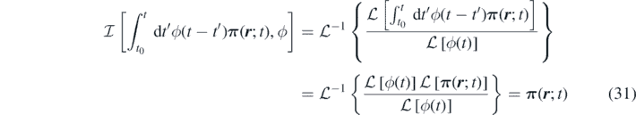
where ![$\mathcal{L}\left[\boldsymbol{\pi }\left(\boldsymbol{r};t\right)\right]{=\int }_{0}^{\infty }\boldsymbol{\pi }\left(\boldsymbol{r};t\right){\mathrm{e}}^{-t/\lambda }\enspace \mathrm{d}t$](https://content.cld.iop.org/journals/1751-8121/53/44/445007/revision3/aab9e8dieqn31.gif) indicates the Laplace transform of a time-dependent field.
indicates the Laplace transform of a time-dependent field.
Applying the operator  in equation (29) for a multicomponent system of ideal gases, we obtain the following non-Markovian time evolution of the density field of the species s:

Neglecting the reaction contributions to the momentum, we obtain:

where we employed the space invariance of the operator  . By utilising equation (31), we obtain
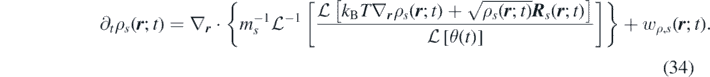
Defining now the function ![$\tilde {D}\left(t\right)={\mathcal{L}}^{-1}\left[{\left(\mathcal{L}\left[\theta \left(t\right)\right]\right)}^{-1}\right]$](https://content.cld.iop.org/journals/1751-8121/53/44/445007/revision3/aab9e8dieqn34.gif) , and using the properties of the Laplace transform we get
, and using the properties of the Laplace transform we get

where ∗ denotes convolution in time.
For a memory kernel in the form  , the function
  is given by

The highest values of λ in the Laplace transform correspond to the lowest frequencies, which are usually dominant. This allows us to simplify the above even further:
Finally, equation (35) reduces to

where we have introduced the effective diffusion coefficient,  .
.
An alternative derivation of equation (38) would be to first take the Markovian limit of an ideal-gas model followed by the overdamped limit assuming that the momentum reaction rate w j ,s is negligible. This way equation (30) would be reduced to the usual reaction–diffusion equation for the density [57]:

In this section we have presented some of the main theoretical results of this work. Using a properly defined deconvolution operator and taking the overdamped limit of the previously derived FH, we derived a novel non-Markovian overdamped FDDFT equation for the density field. Moreover, for memory kernels in the form of exponential series, we simplified the convolutional structure of the above equation, defining an effective diffusion coefficient including low-frequencies contributions to memory effects.
5. Extended field dynamics
Numerically solving the non-Markovian equations (23) and (24) is a highly non-trivial task. First, because it is not obvious how to sample colored (time-correlated) noise. Additionally, the direct evaluation of the convolution integral requires keeping track of the entire history of the momentum field, which drives up the computational cost. Within the so-called extended dynamics approach, additional variables are introduced to capture the memory and noise effects on the observables [56, 62, 63]. In this section we derive the extended dynamics for the non-Markovian FH, generalizing the work by Kawai [63]. For simplicity we assume that the global effects of the bath are isotropic [56] and the memory kernel can be expressed as the exponential series [62, 63] already introduced in section 2 and repeated here for convenience:

5.1. Convolution decomposition
Defining the extended field variable associated with the kth mode of the memory term of species s:

we can express the convolution term as  . By differentiating Zs,k
with respect to t yields the time evolution of the field Zs,k
in the form of a stochastic partial differential equation (SPDE):
. By differentiating Zs,k
with respect to t yields the time evolution of the field Zs,k
in the form of a stochastic partial differential equation (SPDE):

5.2. Noise decomposition
The noise term is given by

where
R
s
denotes the spatial-temporal noise with correlations ⟨
R
s
(
r
; t)
R
s
(
r
'; t')⟩ = kB
Tθs
(t − t'δ(
r
−
r
') I. Notice that because of the symmetry between t and t' in the fluctuation-dissipation theorem, θs
(t) must be even: θs
(t) = θs
(−t). Additionally, its Fourier transform  must be both real and even when ω is real. It follows that in the ω-plane, the roots and singularities of
  must be symmetric with respect to both the real and imaginary axes. This allows us to introduce the function
  such that

where

with real coefficients bs,k
and Bs,k
. The singular points of  lie in the lower half of the complex ω-plane. Moreover, we define two functions in the Fourier space:

and

and we denote their Fourier inverse transform with h(t) and kk (t), respectively. By combining equations (45)–(47) it follows that:

or, equivalently,

Moreover, equation (47) can be rewritten as  , which in the time domain gives:

We introduce two more vector fields, corresponding to a delta correlated stochastic field (as will be proved later) and an auxiliary stochastic field, respectively:

and

From equations (52) and (49) it follows that:

while, combining equations (52) and (50), we obtain

Equations (53) and (54) allow us to express the original correlated noise as a function of the white noise
ξ
(t). A discussion of the properties of the stochastic process
ξ
(
r
; t) can be found in appendix
5.3. Non-Markovian FH equations
Defining an extended field S s,k ( r ; t) = − Z s,k ( r ; t) + η s,k ( r ; t), the FH equations are expressed in the following form:


where
ξ
(
r
1; t1) is a stochastic process with zero mean and correlations  .
.
The system in equation (57) can be also rewritten in vector form:

In the above equation  is the unknown,
  is the conservative flux, and
  is the stochastic term for species s:
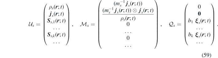
The source terms are
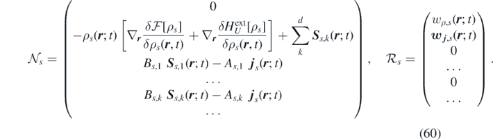
6. Finite volume discretization
The FH system of equations and the corresponding deterministic and overdamped counterparts have been solved numerically using different techniques, including pseudo-spectral methods [64], and finite volumes [57, 65–67]. Here we employ the finite-volume method to discretize equation (58) because of its enhanced capability in dealing with non-regular fields and complex geometries. For simplicity, we present the discretization for a one dimensional system; the generalization to higher dimensions is then straightforward.
A domain of length L is partitioned into n identical cells of width Δx = L/n. The value of the discretized variable vector for the species s at the cell 1 ⩽ j ⩽ n is then defined as the following average over the cell volume Vj

Similarly, time integration is performed by discretizing the total simulation time T in steps of magnitude Δt, such that we can assume  , with 0 ⩽ mΔt ⩽ T. The multiplicative white noise
ξ
s
(
r
; t) is discretized, using the following spatio–temporal average [57, 65]
, with 0 ⩽ mΔt ⩽ T. The multiplicative white noise
ξ
s
(
r
; t) is discretized, using the following spatio–temporal average [57, 65]

where
G
represents a vector with components sampled independently from a standard Gaussian distribution  . In order to implement time stepping, we define the forward and backward conservative fluxes as:

where  denotes the average value of the field
  at the cell j, i.e.

Finally, both source terms are discretized simply:

The source term  contains the gradient of the variation of the free-energy functional. Within mean-field treatment, the latter has the following form:

The above equation can be discretized as follows [66]:

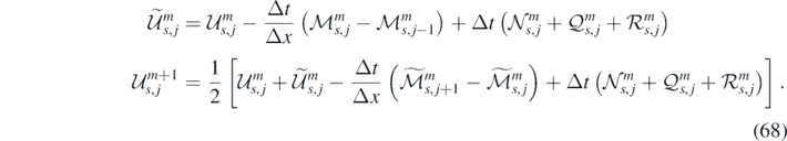
To improve the accuracy of time integration for nonlinear systems, each time step is usually further subdivided. In the present work, we adopt a two-stage MacCormack predictor–corrector scheme [68]:
7. Numerical applications
7.1. Equilibrium mono-component system
In order to test the numerical stochastic integrator, we consider a non-Markovian FDDFT approach to model a system of N non-reacting ideal gas particles with single exponential memory kernel. The particle momentum time correlation function of the corresponding GLE can be obtained in a closed analytical form [62, 69]:
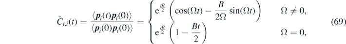
where we introduced a complex-valued parameter  .
.
To obtain the time-correlation function for the discretized non-Markovian FDDFT model, we proceed as follows. First, we define the time-correlation function of the discretized momentum in a cell as:

Next, we employ the independence between p i (t) and r i (t), and between p i (t) and p j (t), to write
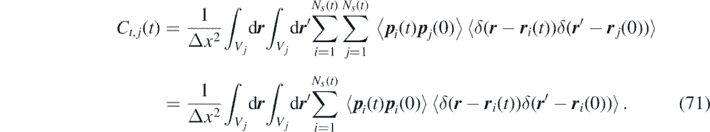
Moreover, since all particles have the same momentum correlation, we introduce Ĉt (t) = Ĉt,i (t). This gives:
Finally, assuming that both r i (0) and r i (t) belong to the same cell Vj , i.e. that the cell size is much larger than the particle mean path, we obtain the time-correlation of the momentum field:
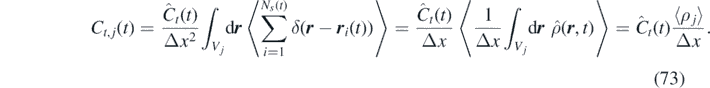
We computed the momentum field time-correlation of a uniform ideal-gas system with non-Markovian FDDFT, atomistic stochastic simulations (GLE) and theory [equation (73)]. The ideal-gas system is coupled with a thermal bath at fixed temperature T = 1 through a single exponential memory kernel. We analyzed systems characterized by three different memory kernels, corresponding to the under damped (A = 1 and B = −1), the damped (A = 1 and B = −2) and the over damped (A = 1 and B = −4) cases. The domain is discretized in 40 cells of Δx = 100 (in reduced units).
The GLE simulations are run with the gld integrator, which is part of the LAMMPS package [62, 70]. The data are gathered over 500 independent trajectories, each running for 104 steps with a time step Δt = 0.001.
The non-Markovian FDDFT is integrated with the finite-volume scheme discussed above. The data are averaged over 1000 independent trajectories, each running for 102 steps with a time step Δt = 0.1.
Figures 2(a)–(c) show that the momentum time-correlation functions obtained using atomistic, continuum and theoretical approaches converge, within statistical uncertainty, to the same result. It is worth noticing that only exponentially decaying momentum time-correlation functions can be obtained in the Markovian approximation, i.e. the time-correlation function in figure 2(a) can be recovered only by means of a non-Markovian framework. We also report the space correlations between every cell and the middle cell for the overdamped case in figure 2(d). Evidently, our numerical scheme does not introduce any spurious space correlations into the ideal gas.

Figure 2. Comparison between numerical and theoretical momentum time-correlations for an ideal-gas system coupled with a thermal bath at fixed temperature T = 1 through a single exponential memory kernel [62]. The time-correlation function is computed in the underdamped limit with A1 = 1 and B1 = −1 (a), in the damped case with A1 = 1 and B1 = −2 (b) and in the overdamped limit with A1 = 1 and B1 = −4 (c). We also report the momentum space correlations between every cell and the middle cell for the overdamped case (d). The system considered is uniform with initial conditions  and
and  . The domain is discretized in 40 cells of Δx = 100.
Download figure:
Standard image High-resolution image7.2. Non-equilibrium space transition
The main aim here is to demonstrate the significant role of the memory kernel in non-equilibrium processes and to validate the FH algorithm using GLE simulations. We study an ideal-gas system at temperature T = 1 inside the double-well potential:

with C = 5 and x0 = 200. The time evolution of the system is computed in the underdamped limit, with A1 = 1 and B1 = −1, and in the overdamped limit, with A1 = 1 and B1 = −4. To force mass transport between the two wells, the system has non-uniform initial conditions with  ,
,  , where
  refers to the density in the left well and
  to the density in the right well. As in the previous example, the GLE simulations are run with the gld integrator. The data are gathered over 10 independent trajectories, each running for 109 steps with a time step Δt = 0.001.
The non-Markovian FDDFT is integrated with the finite-volume scheme discussed above. The data are averaged over 100 independent trajectories, where each was run for 106 steps with a time step Δt = 0.1.
Figures 3(a) and (b) depict a comparison of the time-evolution of the mean density profiles obtained from GLE and FH in the underdamped and overdamped cases. Despite the presence of a sharp gradient, the numerical scheme is able to accurately reproduce the diffusion of the density step function and the mass transfer between the two wells. The evolution in time of the difference between the total mass contained in the left well m+(t) and the mass in the right well m−(t) is reported in figure 3(c). The noticeable difference between the overdamped and underdamped cases highlights the importance of the memory effects when modeling out-of-equilibrium systems. This prototypical example suggests that, during phase transitions, but also biological state transitions and chemical reactions, the widely adopted Markovian assumption may not be satisfied.

Figure 3. Comparison between FH and GLE for a non-uniform ideal gas in a double-well potential at temperature T = 1. The system is started off with a non-symmetric initial condition to force mass transport between the two wells. The density-time evolution is computed in the underdamped limit with A1 = 1 and B1 = −1 (a) and in the overdamped limit with A1 = 1 and B1 = −4 (b). In (c) we report the time evolution of the difference between the total mass contained in the left well m+(t) and the mass in the right well m−(t). Such dynamics clearly shows the significant influence of the memory kernel on non-equilibrium processes. The domain is discretized in 40 cells of Δx = 10 and periodic boundary conditions are used.
Download figure:
Standard image High-resolution image7.3. Memory-driven Turing patterns in binary reacting system
Here we apply our framework to study Turing patterns [43] observed in reaction–diffusion systems. Specifically, our aim is to show how Turing patterns can arise in systems composed of two reacting chemicals characterized by dissimilar memory kernels. To observe Turing patterns in two-component systems one typically needs to use a third substance, which is fixed in space and reversibly bound to only one of the two components. As a result, the effective diffusion coefficient of the binding component is significantly smaller than that of the other components. Here we show that a similar scenario can be realized by using a thermal bath with dissimilar memory kernels for the two reacting components.
Consider the non-linear kinematic chemical-kinetics model proposed by Schnakenberg [44] involving three reactions with chemicals X1, A, B and X2:

with k−1, k1, k2 and k3 representing the reaction-rate constants. This reaction involves an autocatalyst X1 (it is both product and catalyst) for the same elementary reaction, a reactant X2 and two auxiliary species A and B, which are later assumed in excess. The prototypical Schnakenberg's reaction model exhibits interesting dynamical behaviors (i.e. steady-state solutions with spatially inhomogeneous patterns and bifurcations [71]). It also has many direct applications in the study of morphogenetic processes involving skin patterns [72]. Let us define the densities of X1, A, B and X2 as ρ1, α, β and ρ2, respectively. The law of mass action states that the rate of a chemical reaction is proportional to the concentration of the reacting species. This law, when applied to equation (75), gives the time-evolution of the components, namely:
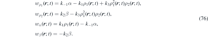
If A and B are in excess, then α and β can be assumed to be constant. It follows that wα ( r ; t) ∼ wβ ( r ; t) ∼ 0, the so-called 'quasi-steady approximation' in chemical kinetics, and the following system of continuity equations governs the time evolution of the system:

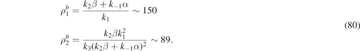
The following parameters are adopted in our numerical simulations: k−1 α = 1.0, k1 = 0.02, k2 β = 2.0, k3 = 10−6.
Turing patterns are observed when a uniform dynamical system is linearly stable in the absence of diffusion, but becomes linearly unstable in the presence of non-uniform diffusion. In our analysis, we use the one-dimensional overdamped density equation, equation (38), in the weak-noise limit:

where we defined  and
and  . First, we compute the stationary states of the Schnakenberg model by setting:

A unique uniform stationary state then exists given by:
The Jacobian matrix for the purely reactive system evaluated at the stationary state, i.e. with components  , is given by:
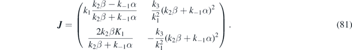
At the same time, the Jacobian matrix of the reaction–diffusion system is given by J k = J − [d1, d2] I . The reaction parameters chosen in this study satisfy the following conditions


to ensure the stability of the purely reactive system, as required for the appearance of Turing patterns (see appendix
The effective diffusion parameters d1 and d2 are functions of the memory kernels, as shown in section 4. We consider two cases, both with single exponential memory kernels, with parameters A1,1 = 1.0, A2,1 = 1.0 and B2,1 = −20.0. The two cases differ due to B1,1, which is set to = −0.4 in case (a) and to −0.2 in case (b). The respective values of d1 are 0.4 and 0.2. Notice that in both cases the Turing instability conditions are satisfied because De tJkm
< 0 (see appendix

Such value corresponds to a wave-length L = 2π/km .
Figure 4 shows the time-evolution of the density for case (a) obtained from both deterministic and stochastic formulations. The characteristic wavelength for such a system, L ∼ 70, is theoretically predicted by equation (84) and is recovered in both deterministic and stochastic solutions. As expected, for the stochastic evolution the instability is enhanced by the noise, thus the patterns arise sooner. Interestingly, the structure factor reported in figure 5 and discussed in appendix

Figure 4. Turing patterns for B1,1 = −0.4 characterized by a wavelength L ∼ 70 consistent with the one predicted theoretically. Panels (a)–(c) and (b)–(d) correspond to the deterministic and stochastic cases, respectively. Panels (a) and (b) and (c) and (d) show the evolution in time of the densities of the two components ρ1 and ρ2, respectively.
Download figure:
Standard image High-resolution image
Figure 5. Turing patterns for B1,1 = −0.4 characterized by a wavelength L ∼ 70 consistent with the one predicted theoretically. Panels (a)–(c) and (b)–(d) correspond to the deterministic and stochastic cases, respectively. The steady-state densities are reported in (a) and (b). In (c) and (d) we plot the structure factors of the steady states.
Download figure:
Standard image High-resolution imageIn figure 6 we report the deterministic and stochastic density evolution for case (b). In this case we also observe the wavelength predicted by the theoretical analysis, L ∼ 50. However, the evolution of this system shows the presence of secondary peaks with low intensity, as also suggested by the corresponding structure factor (figure 7).

Figure 6. Same as figure 4, but for B1,1 = −0.4 and L ∼ 50.
Download figure:
Standard image High-resolution image
Figure 7. Same as figure 5, but for B1,1 = −0.4 and L ∼ 50.
Download figure:
Standard image High-resolution imageLet us conclude this section by emphasizing that the prototypical Schnakenberg model was used to exemplify our FFDFT framework. But the framework is quite general and can be used to model any reaction scheme. Specifically, obtaining the memory kernel for each species (via e.g. molecular dynamics simulations) opens the road to analyzing the influence of interparticle interactions and correlated fluctuations (accounting for thermal bath effects) on pattern formation.
8. Summary and conclusions
We have derived a theoretical–computational framework for reactive multispecies colloidal systems. Starting from the non-Markovian GLEs describing the motion of the reactive particles, and by appropriately defining the local number and momentum density fields, we obtained the corresponding non-Markovian Navier–Stokes-like system of microscopic FH. Introducing the Helmholtz free-energy functional from classical density-functional theory yields a non-Markovian FDDFT for reacting multispecies fluid systems, the main result of our theoretical work. Introducing an appropriate deconvolution operator enables us to obtain the overdamped limit. This resulted in the non-Markovian and overdamped equation for the density field, a generalisation of FDDFT to include chemical reactions and memory effects. Moreover, in order to make the equations for the non-Markovian FDDFT computationally tractable, we introduced additional field variables whose purpose is twofold: they include the memory term contributions without actually computing any convolution explicitly, and they account for the effects of the time-correlated random term. This additional fields allowed us to develop an extended dynamics framework equivalent to the non-Markovian FDDFT. Additionally, we presented a finite-volume scheme to discretize the non-Markovian FDDFT, and we provided several numerical experiments to exemplify our framework. These include ideal gas in-and-out-of equilibrium, and a two-species reacting system exhibiting memory-driven Turing patterns.
The framework can be adopted to investigate a wide spectrum of physicochemical phenomena in colloidal systems. We have demonstrated that memory effects, through inducing time correlations and variations of the fluid mobility that alter the transition path, can play a crucial role in the dynamical evolution of systems undergoing state transitions. As a result, the theoretical–computational treatment of memory effects requires careful consideration.
We believe that our results can motivate further theoretical–computational studies on reactive colloidal systems and may even be useful in the experimental scrutiny of pattern formation including Turing patterns. There are also a number of interesting questions related to the work presented here. For example, an interesting extension would be to apply the methods proposed here to the study of phase transitions in biological fluids where memory effects should play an important role. Such systems are often characterized by space- and time-scales, which are not accessible with atomistic simulations [7, 8]. Another possible line of future work is to include the effects of geometric confinement [73–75]. We shall examine these and related issues in future studies.
Acknowledgments
We gratefully acknowledge financial support from the Imperial College (IC) Department of Chemical Engineering PhD Scholarship scheme, European Research Council through Advanced Grant No. 247031 and the Engineering and Physical Sciences Research Council of the UK via Grants No. EP/L027186 and EP/L020564. The computations where performed at the High Performance Computing center of IC. Finally, we are grateful to the anonymous referees for insightful comments and suggestions.
Appendix A.: Derivations of noise in fluctuating hydrodynamics
The noise term in equation (10) is  , where
R
i,s
(t) has zero mean and correlation function ⟨
R
i,s
(t)
R
i,s
(t')⟩ = kB
T
θ
s
(t − t'). It follows that the spatiotemporal correlations of
η
s
can be expressed as:
, where
R
i,s
(t) has zero mean and correlation function ⟨
R
i,s
(t)
R
i,s
(t')⟩ = kB
T
θ
s
(t − t'). It follows that the spatiotemporal correlations of
η
s
can be expressed as:

Using the property of the Dirac delta function
the spatio–temporal correlations of ηs can be rewritten as:
Thus, introducing a spatiotemporal noise satisfying ⟨ R s ( r ; t) R s ( r '; t')⟩ = kB T θ s (t − t')δ( r − r '), the local fluctuation term can be rewritten as

Appendix B.: Stochastic process of extended field dynamics
In this section, we discuss the properties of the stochastic process
ξ
(
r
; t). First, since all the singularities of  lie in the lower-half complex ω-plane, then for τ > 0:
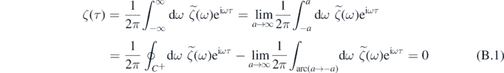
where  indicates the integral over a closed contour C+ that goes along the real line from −a to a and then along a semicircle centered at 0 from a to a, while ∫arc(a→−a)dω is the integral along an arc centered at 0 from a to −a. Hence, for t > 0 we can write

Thus, the spatio–temporal correlation function of ξ s ( r ; t) is given by:
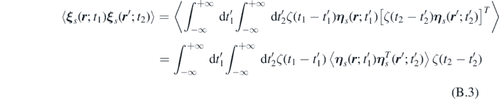
where we used the fluctuation-dissipation theorem.
Employing the definition of Fourier transform of θs and ζ(t), together with equations (44)–(46), we obtain:
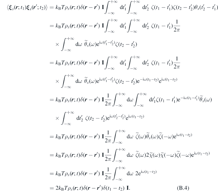
It follows that ξ s ( r ; t) is delta-correlated in space and time, and consequently can be easily generated, i.e. as in reference [65].
Appendix C.: Linear stability analysis for reaction–diffusion systems
Turing patterns are observed when a uniform system is stable in the absence of diffusion, but become unstable to perturbation with diffusion. For the analysis, we consider the one-dimensional density equation:

with stationary states given by:

Hence, we study the linear stability of the system around the stationary state for both the corresponding reacting-only system and for the full system. The time evolution of the infinitesimal perturbations δρ1 and δρ2 is given by:

where the coefficients of the Jacobian matrix evaluated at the stationary state  are introduced. A particular solution is given by

Combining equations (C.3) and (C.4), we obtain the eigenvalue problem:

where

The uniform stationary solution is stable if both eigenvalues λk,i at a wave number k have negative real part. Such a condition is verified if:


Turing patterns can arise when a reaction-only system, corresponding to d1 = d2 = 0, is stable, but the corresponding reaction–diffusion system is unstable. The reaction-only system is stable when the following two conditions are satisfied:


The reaction–diffusion system is unstable when at least one of equations (C.7) and (C.8) is not verified. Because of equation (C.9), Tr Jk < Tr J < 0, thus equation (C.7) is always verified. Instability then occurs if and only if Det Jk < 0 for at least a value of k. The minimum value of k for which such a condition occurs is given by:

which corresponds to a wave number Lk = 2π/k. It directly follows that the corresponding Det Jkm < 0 when:

Appendix D.: Structure factor
As shown in previous works [57, 65], the structure factor is useful not only to study the stability of the numerical integrator, but also in multi-phase systems to obtain the frequency components characterizing the system. If we consider a periodic domain of volume V, the spatial Fourier transform of the number density for the species s is given by:

Thus, the structure factor is defined as the variance of the Fourier transform of the density fluctuations of species s,

with the Fourier transform of the density fluctuations being  . In case of uniform ideal gases, the structure factor is computed as [57]:

Footnotes
- 1
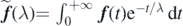
The Laplace transform of a function f (t) is defined as
 .
.