
Abstract
For a one-dimensional Schrödinger operator with a finite number n of point delta-interactions with a common intensity, the parameters are the intensity, the n − 1 intercenter distances and the mass. Critical points are points in the parameters space of the Hamiltonian where one bound state appears or disappears. The study of critical points for Hamiltonians with point delta-interactions arranged along a Fibonacci chain is shown to be closely related to the study of the so-called Fibonacci operator, a discrete one-dimensional Schrödinger-type operator, which occurs in the context of tight binding Hamiltonians. These critical points are the zeros of orthogonal polynomials previously studied in the context of special diatomic linear chains with elastic nearest-neighbor interaction. Properties of the zeros (location, asymptotic behavior, gaps, ...) are investigated. The perturbation series from the solvable periodic case is determined. The measure which yields orthogonality is investigated numerically from the zeros. It is shown that the transmission coefficient at zero energy can be expressed in terms of the orthogonal polynomials and their associated polynomials. In particular, it is shown that when the number of point delta-interactions is equal to a Fibonacci number minus 1, i.e. when the intervals between point delta-interactions form a palindrome, all the Fibonacci chains at critical points are completely transparent at zero energy.
Export citation and abstract BibTeX RIS
1. Introduction
Fibonacci chains are the most simple models for one-dimensional quasi crystals, see e.g. [1]. They are the subject of a large number of theoretical works, mostly within the framework of chains with nearest-neighbor interaction, see e.g. [2–12]. Most of these studies are concerned with infinite chains.
This paper is concerned with critical points of a Hamiltonian with a finite number of point delta-interactions whose distances are distributed along a Fibonacci chain. By point delta-interactions, it is meant interactions described by Dirac distributions. For precise mathematical definitions of point delta-interactions in terms of self-adjoint extensions of operators, see [13]. It is stressed that point delta-interactions are not nearest-neighbor interactions. Critical points then are points in the parameters space of the Hamiltonians where one bound state appears or disappears. The study of critical points for Hamiltonians with point delta-interactions is shown to be closely related to the study of the so-called Fibonacci operator [2–12], a discrete one-dimensional Schrödinger-type operator, which occurs in the context of tight binding Hamiltonians [2–7] or elastic nearest-neighbor interaction [8–10]. These critical points are the zeros of orthogonal polynomials. These polynomials have been introduced and studied previously in the context of special diatomic linear chains with elastic nearest-neighbor interaction and the two masses distributed according to a Fibonacci sequence [8–10].
Section 2 defines precisely the Hamiltonians with a finite number of point delta-interactions distributed along a Fibonacci chain, and shows that the critical points are determined as the zeros of orthogonal polynomials previously introduced and studied in [8–10]. General properties of these orthogonal polynomials (excluding the study of the zeros) are given in section 3. The study of the critical points, i.e. of the zeros of the orthogonal polynomials, is the subject of section 4. In particular, subsection 4.10 investigates the measure of orthogonality of polynomials from the numerically computed zeros. Section 5 investigates transmission coefficients at zero energy. Subsection 5.1 shows that the transmission coefficient at the limit of zero energy is zero except for a Fibonacci chain at critical points. Subsection 5.2 shows complete transparency at zero energy of all critical Fibonacci chains when the number of centers is a Fibonacci number minus 1.
2. The Hamiltonian and its critical points
Fibonacci chains can be defined via the substitution s acting on two letters A, B, and defined by


Starting from B (step 0), one obtains successively s(B) = A (step 1), s2(B) = AB (step 2), s3(B) = ABA (step 3), s4(B) = ABAAB (step 4), ... . It is important to note that the steps can also be constructed by concatenations: step i followed by the step i − 1. For example, step 4, ABAAB, is obtained by writing first step 3, ABA, and then, on the same line, step 2, AB. As a result, the number of letters at step i is equal to the Fibonacci number Fi + 1 defined recursively by Fn = Fn − 1 + Fn − 2 with F0 = 0, F1 = 1. (Care should be taken with the notation. In particular, some authors consider Fi as the present Fi + 1.)
Up to now, we have used the term Fibonacci chain in a rather general sense, and from now on it will have a very specific and restricted meaning. Let us first define what we mean by a Fibonacci word of n letters throughout this paper.
Definition 1. A Fibonacci word of n letters in the alphabet A, B is the first n letters (from left to right) of the sequence obtained from iteration of the substitution s defined by (1a), (1b). This word is denoted as Wn(A, B) or, if n is unspecified, W(A, B).
Thus, n can be an arbitrary positive integer. For example, according to this definition, ABAA is a Fibonacci word of length 4, whereas BAABA is not a Fibonacci word because it is obtained from a Fibonacci sequence by truncation from the left.
For the one-dimensional Hamiltonian

with n Dirac δ interactions centered at the n distinct points yj, it has been shown [15] that the critical points are the roots of the determinant of an (n − 1)th-order tridiagonal matrix T(n − 1) whose non-zero elements are

with j = 1, ..., n − 1 and dj, the distance between centers defined by

We use units for which ℏ = 1. The Hamiltonian considered in this paper is a particular case of (2):

where μ is a negative strength interaction parameter common to all n centers.
Definition 2. The term Fibonacci chain of n centers denotes Hamiltonian (5) where the n − 1 distances d2, d3, ..., dn form a Fibonacci word Wn − 1(τf, f), with f a fixed length and τ dimensionless. The conditions μ < 0 and τ > 0 are assumed.
Specifically,

where uj is defined in appendix A by (A.7) (or equivalently (A.8)–(A.12)). At this stage, it is necessary to introduce a few notations that will be used in all the paper. The floor of x, i.e. the greatest integer less than or equal to x, will be denoted as ⌊x⌋. Some useful properties of Fibonacci words and their relations to the golden ratio

are given in appendix A. Some results of appendix A could be obtained more rapidly from known properties of so-called Wytoff A and B sequences [14] and of the so-called rabitt sequence [14]. The results of appendix A will be used freely from now on, and therefore it may now be appropriate to have a brief look at them. As noted in appendix A, the sequence uk (A.7) is the Fibonacci sequence ABAAB⋅⋅⋅ with 1 for A and 0 for B. The sequence  therefore is the Fibonacci sequence ABAAB⋅⋅⋅ with τ for A and 1 for B. Thus,
  . Of course, for τ = 1, all the intervals dj + 1 are equal (finite uniform chain).
The tridiagonal matrix μT(n − 1) then has for non-zero matrix elements

With

one therefore has

For example,
It is a remarkable fact that the critical points depend only on x given by (9). To summarize, μT(n) is an n-order real symmetric tridiagonal matrix, whose non-zero nondiagonal elements are minus unity, and diagonal elements form a Fibonacci word Wn(2(1 + xτ), 2(1 + x)). The determinant of μT(n − 1) will be denoted as Qτn − 1(x), and it is clear that Qτn is a polynomial of degree n. The critical points of the n centers, Hamiltonian (5), thus are the zeros of the (n − 1)th-order polynomial Qτn − 1(x) to be discussed in the next section.
Definition 3. A critical Fibonacci chain of n centers is a Fibonacci chain of n centers at a critical point, i.e. having for a value of the parameter x (9) a zero of Qτn − 1.
Thus, from a Fibonacci chain of n centers, n − 1 critical Fibonacci chains can be constructed, since it will be seen that the zeros are distinct.
3. The orthogonal polynomials
3.1. Recursion relations
By Laplace expansion of the determinant Qτn along its last column, one has the recursion relation (12a)


It is then easy to verify by explicit calculation of Qτ1(x) that the recursion relation (12a) together with definitions (12b) corresponds to the determinant of μT(n). (12a) gives for the coefficient of xn in Qτn, 2n(u1 + u2 + ⋅⋅⋅ + un) = 2nτ⌊(n + 1)/g⌋ where the last equality comes from (A.13). Also (12a) gives for the coefficient of x0 in Qτn, n + 1.
The first explicit expressions (n = 1, 2, 3) are


The polynomials Qτn(x) have been introduced and studied previously [8–10]. In the notations of [9], Qτn(x) is denoted as S(r)n( − x) or Sn(2(1 + rx), 2(1 + x)) with r = τ. The viewpoint of polynomials in the two variables x and xτ is of particular interest when looking for a generating function of these polynomials [8–10]. In the present paper, we have tried to use notations similar to the general notation of [17]. The polynomial proportional to Qτn(x), whose coefficient of the highest degree xn is unity, i.e. the corresponding monic polynomials, will be denoted as  . It is then easy to show that the monic polynomials are completely determined by


In fact, λτ1 can be chosen arbitrarily without changing  , but the choice λ1 = 1 will be convenient for subsequent normalization of a measure. The sequence
  , {n = 1, 2, ...} is a Fibonacci sequence ABAA... with
  and B = 1. The sequence λτn, n = 2, 3, ... (note that n starts at 2, not 1), is a Fibonacci sequence ABAA⋅⋅⋅ with
  (the juxtaposition, not the product), and
  (see appendix A). It is a theorem known as the Favard theorem [17, 18] that if the coefficient
  of
of  in (14a) is real and λτn > 0 for n ⩾ 1, the
  form an orthogonal polynomial sequence (OPS) with respect to a unique, positive definite functional
  ,
,


with δmn the Kronecker symbol equal to 1 if m = n, 0 otherwise. The present  and λτn clearly satisfy the conditions required in the Favard theorem since τ > 0. As with every OPS, one can associate with the polynomials
  other monic polynomials
  , known as associated or numerator polynomials defined by


which also constitute an OPS, but relative to a different functional,  '. It will be seen in section 5.1 that both Qτn and Rτn are involved in the expression of the transmission coefficient at zero energy. Introducing the matrix [2–12]

it will be of interest to put (12a) and (12b) into the matrix form,
where Rτn(x) is a polynomial proportional to  , defined by


The determinant of Φτn is unity since it is the product of Tτk matrices whose determinant is unity. Different relations between the polynomials Qτn and Rτn are given in [9] and [11]. Another one, which will be useful in section 5, is

A proof of (21) relies on the fact that the Fibonacci words  of Fk − 2 letters are palindromes. A proof of this palindromic property based on concatenations is given in [20]. Another proof, based on substitutions (1a) and (1b), is given in appendix B. Palindromes are words equal to the reversed words. For example,
  ,
,  ,
,  ,
,  . The palindromic property can equivalently be formulated algebraically:

We now prove (21). Introducing the Pauli matrix

and considering (19), (21) is equivalent to Tr(σ1ΦτFk − 2) = 0 with the symbol Tr for the trace. Due to the palindromic property,

where X is the identity matrix if Fk − 2 is even and Tτi otherwise. Since σ21 is the identity matrix,

Since σ1Tτmσ1 = (Tτm)−1, by using the invariance of the trace by circular permutations, one obtains

The process can be iterated up to Tr(σ1ΦτFk − 2) = Tr(σ1TτjXTτj). If X is the identity matrix, this reduces to Tr(σ1ΦτFk − 2) = Tr(σ1) = 0. If X = Tτi, iteration of the process gives Tr(σ1ΦτFk − 2) = Tr(σ1Tτi) = 0. Thus, (21) is finally proved.
For τ = 1, (19) reduces to

with Un the Chebyshev polynomial of second kind defined by Un(cos θ) = sin [(n + 1)θ]/sin θ.
We also give defining relations for orthonormal (with respect to the functional  ) polynomials qτn(x) proportional to
  , and orthonormal (with respect to the functional
  ') polynomials rτn(x) proportional to
  [17],
[17],


The orthonormal polynomials qτn(x) will be used later (60) for numerical investigation of the measure of orthogonality. As a result, these orthonormal polynomials are completely determined by


3.2. Christoffel Darboux identities


3.3. Continued fractions
Let us consider the continued fractions  defined by
  and An = bnAn − 1 + anAn − 2, A−1 = 1, Bn = bnBn − 1 + anBn − 2, B−1 = 0 with bi ≠ 0 for i ⩾ 1. Then with b0 = 0, a1 = λ1, and an + 1 = −λn + 1, bn = x − cn for n > 1, we have qτn(x) = Bn, rτn(x) = (λ1τ)−1An + 1 (hence the other name numerator polynomial for the associated polynomial). For more details and other properties shared by all orthonormal polynomials, see [17–19].
3.4. Connection with the Fibonacci operator
The so-called Fibonacci operator [2–12] is a discrete one-dimensional Schrödinger-type operator, which occurs in the context of tight binding Hamiltonians. Let |n〉 be an orthonormal basis in some Hilbert space and let H be the Hamiltonian defined by H|n〉 = |n + 1〉 + |n − 1〉 + αun|n〉 with un defined by (A.7) and α > 0. Then the Schrödinger equation H|ψ〉 = z|ψ〉 with |ψ〉 = Σnan|n〉 gives for the sequence  , an + 1 + an − 1 + αunan = zan. By comparison with (10) it is clear that −μT(n − 1) has the same matrix elements as H − z with z = 2(1 + x) and α = −2x(τ − 1). Therefore, some results obtained for the Fibonacci operator [2–12, 16] can be translated in the present context. In particular, defining Ξτn ≡ ΦFnτ and
  , one has Ξτn + 1 = Ξn − 1τΞτn, sτn + 1 = 2snτsτn − 1 − sn − 2τ, (sτn + 1)2 + (snτ)2 + (sτn − 1)2 − 2sn + 1τsτnsn − 1τ − 1 = x2( − 1 + τ)2.
4. The zeros
It is recalled that the zeros are the critical points. Some well-known important general results are briefly recalled in sections 4.1 and 4.3. More specific results are presented in sections 4.2 and 4.4–4.10.
4.1. General properties of zeros of orthogonal polynomials
The zeros of qτn and those of rτn are simple. Throughout this paper, the n zeros xτn, i, i = 1, ...n, of qτn will be noted in increasing order:

Then we have the interlacing properties [17] xτn + 1, j < xn, jτ < xτn + 1, j + 1. The same inequality holds for the zeros yτn, i of rτn [17]. Moreover [17], xτn + 1, j < yn, jτ < xτn + 1, j + 1.
4.2. The zeros are negative
Subtract Qτn − 1(x) from both members of (12a) and sum over n. One obtains
With k = 1, (35) shows that the coefficients of every power of x are positive for the polynomials Qτ1(x) since Qτ0(x) = 1 (recall that τ > 0). Then, by recursion on k, (35) shows that the coefficients of every power of x are positive for Qτk(x) whatever the value of k. Recalling that the zeros are real, the zeros of a polynomial with positive coefficients cannot be positive. Since Qτk(0) ≠ 0, the zeros are negative.
It is known [15] that μ in (5) should be negative in order that the Hamiltonian supports bound states. What has been done in this section is the proof using only the definition of the polynomials.
4.3. The zeros as eigenvalues
The zeros xτn, i of qτn are the eigenvalues of a tridiagonal symmetric real matrix Mτn of order n whose non-zero elements are [17]  . Indeed, the Laplace expansion along the last column of
  corresponds to (14a) and (14b). This gives another proof that the zeros are real. For example,
The zeros yτn, i of rτn are the eigenvalues of a tridiagonal symmetric real matrix Nτn of order n whose non-zero elements are

4.4. The zeros are increasing functions of τ and do not cross
The important property in the title of this section can be derived along the framework of the Hellmann–Feynman theorem. Let the ith zero xτn, i be considered as a function of τ. Let w be a normalized real column eigenvector belonging to the zero eigenvalue of the real symmetric matrix μT(n) (10), and take the total derivative of wtμT(n)w = 0 with respect to τ (wt is the transpose of w). The sum  yields zero because T(n)w is the null vector (another argument is that wtw = 1 and w is an eigenvector), and it remains

Now  is a diagonal matrix with diagonal elements equal to 2 or 2τ and therefore
  . Similarly,
  is a diagonal matrix with diagonal elements equal to 0 or 2xτn, i and therefore
  . One therefore deduces from (37) that

Two different zeros xτn, i, xτn, j (i ≠ j) cannot cross since all the zeros are simple.
4.5. First general results about the location of the zeros
For the sum Στn := ∑k = 1nxτn, k of the zeros, i.e. minus the coefficient of xn − 1 in  , one obtains either directly from (14a), or by noting that this sum is the trace of Mτn,

The evaluation of the last sum is obtained using (A.13) and (A.14). For other results concerning sums of powers of roots, see [21].
The product Πτn of the zeros can be obtained from the expression of the coefficients of highest power xn and constant term x0 indicated above (13a). Therefore,

Note that (40) is also the determinant of Mτn.
The sum of the absolute values of matrix elements belonging to the same line of the tridiagonal symmetric matrix Mτn can only be one of the following:  . Then by a general theorem [22, 23], the spectral radius of Mτn is less than or equal to the maximum of these numbers, and therefore
Figure 1 shows the zeros as a function of τ for n = 100. The dashed line curve at the bottom represents the lower bound (41). There is only two different diagonal matrix elements for Mτn, namely −1/τ and −1. The maximum radius of the Geršgorin disk centered at −1 is  , and the maximum radius of the Geršgorin disk centered at −1/τ is
  if τ ⩽ 1 and
  if τ ⩾ 1. Therefore, for τ ⩽ 1 the union of all Geršgorin disks is a disconnected set if and only if
  , i.e. if
  . Also, for τ ⩾ 1 the union of all Geršgorin disks is a disconnected set if and only if
  , i.e. if
  . It remains to count the number of centers −1 and the number of centers −1/τ to find the number of zeros of Qτn in each component of the disconnected set. Since the diagonal elements of Mτn form a Fibonacci word Wn( − 1/τ, −1), (A.13) and (A.14) give the following.
- Case
 : in the interval , there are zeros. In the non-overlapping interval , there are zeros.
 - Case : in the interval , there are zeros. In the non-overlapping interval , there are zeros.
![$\big[{-}\frac{1}{\tau }- \frac{1}{2}\big(\frac{1}{\tau }+ \frac{1}{\sqrt{\tau }}\big),-\frac{1}{\tau }+ \frac{1}{2}\big(\frac{1}{\tau }+ \frac{1}{\sqrt{\tau }}\big)\big]$](https://content.cld.iop.org/journals/1751-8121/44/42/425302/revision1/jpa392985ieqn48.gif)

![$\big[-1- \frac{1}{\sqrt{\tau }},-1+ \frac{1}{\sqrt{\tau }}\big]$](https://content.cld.iop.org/journals/1751-8121/44/42/425302/revision1/jpa392985ieqn50.gif)

![$\big[{-}\frac{1}{\tau }-\frac{1}{\sqrt{\tau }},-\frac{1}{\tau }+ \frac{1}{\sqrt{\tau }}\big]$](https://content.cld.iop.org/journals/1751-8121/44/42/425302/revision1/jpa392985ieqn53.gif)

![$\big[{-}1- \frac{1}{\sqrt{\tau }},-1+ \frac{1}{\sqrt{\tau }}\big]$](https://content.cld.iop.org/journals/1751-8121/44/42/425302/revision1/jpa392985ieqn55.gif)

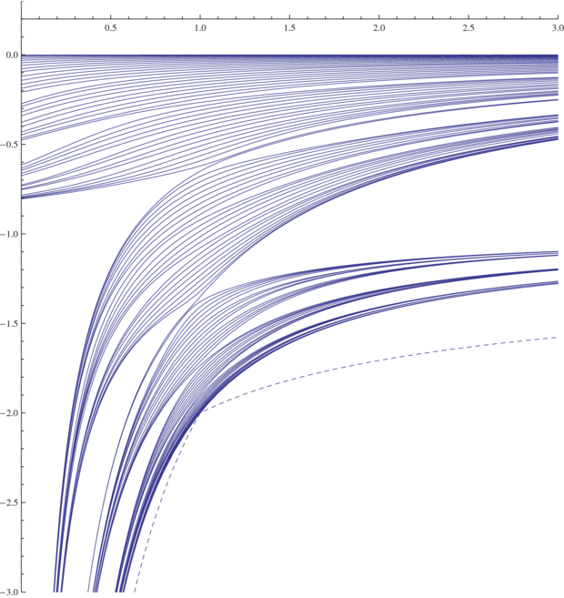
Figure 1. AbscissA: τ. Ordinate: the 100 zeros xτ100, i of Qτ100. The dashed line curve at the bottom represents the lower bound (41).
Download figure:
Standard image4.6. Perturbation series around τ = 1
The case τ = 1 corresponds to an equidistant linear chain. The zeros at τ = 1 are exactly known

with k = 1, ..., n. They are the zeros of the Chebyshev polynomials Un(1 + x). We shall see in section 4.6.2 that the series of xτn, i in integer powers of τ − 1 can be expressed in a compact form and calculated to any finite order k. The first-order perturbation correction is first calculated in the traditional way in section 4.6.1.
4.6.1. First-order correction around τ = 1
For a finite periodic chain, i.e. for τ = 1, the critical points (zeros of Q1n or equivalently eigenvalues of M1n) are known analytically (42), and the same holds for the eigenvectors of M1n. Indeed, let en, k, k = 1, ..., n, denote the normalized column eigenvector corresponding to the eigenvalue x1n, k .They are orthogonal as eigenvectors of a real symmetric matrix. It can be verified that en, k has, within arbitrary global phase factors, the components ejn, k, j = 1, ..., n:
To first order in  , one has M1 + n = Mn1 + Cn with Cn a tridiagonal real symmetric matrix whose main diagonal elements form a Fibonacci word Wn(, 0), and whose elements of the two other non-zero diagonals form a Fibonacci sequence with
  (juxtaposition) and
  (see appendix A). For example,
The first-order perturbation theory yields to first order in
The tridiagonal symmetric structure of Cn allows us to break these sums into two parts: one concerning the main diagonal and the other concerning the two other diagonals. In order to minimize the number of summation terms for the main diagonal, we first evaluate it for the case where all diagonal elements are , which gives a contribution of , and then subtract the contribution of only the zero diagonal elements which are replaced by . The largest integer k such that ⌊kg2⌋ ⩽ n is  (see appendix A). The first part is then
The same procedure can be applied to the two other diagonals by first considering all elements equal to  and then correcting for the contribution of the elements equal to
  . Since the largest integer k such that ⌊⌊kg2⌋g⌋ ⩽ n is
  (see appendix A), one obtains
Using the trigonometrical relation,

and putting all results together, one finally obtains to first order in

The presence of the floor function in (44) is at the origin of the onset of fractal aspect as soon as τ departs from unity.
4.6.2. Higher order corrections to the critical point around τ = 1
Let us first give a relation that allows us to calculate the derivative of the zeros xτn, i with respect to τ using only the knowledge of the zeros. Taking the total derivative with respect to τ of Qτn(xn, iτ) = 0, one obtains
where  and
and  are evaluated at x = xτn, i. This is a first-order differential equation satisfied by xτn, i. Since the value of x = x1n, i is known, (45) is also a sufficient relation that also allows us to determine xτn, i. Now, the first-order coefficient c1, n, i (44) can also be computed as

More generally, the coefficients ck, n, i of the power series

can be expressed as

where the right member is to be evaluated at τ = 1. It is stressed that in (48), the derivatives are the total derivatives with respect to τ. For example,

Equation (48) provides a direct algorithm for the computation of the coefficients of the Rayleigh–Schrödinger perturbation series (47). Figure 2 shows the power series (48) truncated with a maximum value of k equal to 5 for the case n = 10.
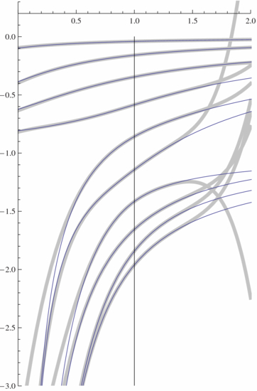
Figure 2. AbscissA: τ. Ordinate: the ten zeros xτ10, i of Qτ10. The thin curves represent numerical results for xτn, i, the thick gray curves represent the truncated power series (47) 0 ⩽ k ⩽ 5.
Download figure:
Standard image4.7. The asymptotic behavior τ → 0
There are only two values for the non-zero nondiagonal matrix elements of M(n), namely 1/(2τ) and  . For τ near zero, it is therefore natural to consider as a zero-order starting point the matrix M(n)0 obtained from the matrix M(n) by replacing the nondiagonal matrix elements
  by zero. In the limit n → ∞, the resulting matrix M(n)0 is block diagonal, with block submatrices of order 1 or 2. The submatrices of order 1 have for matrix elements either −1/τ or −1, and the block submatrices of order 2 are all equal to

whose eigenvalues are −3/(2τ) and −1/(2τ). If n is such as the block submatrix of order 2 is truncated, it becomes a one-order matrix of matrix element equal to −1/τ. To summarize, this zero-order approximation yields only four zeros, namely

Since this zero-order approximation M(n)0 leads to only four eigenvalues, it remains to give the degrees of degeneracy yi of each eigenvalue xi. The number of −1 diagonal elements of M(n)0 is the same as M(n), and therefore  (A.14). The number of elements of the upper diagonal of Mn is n − 1 and using (A.22),
  . The difference between n and the previous degrees gives the degeneracy degree of the remaining value −1/τ:
  . Figure 3 shows the four zero-order approximation zeros (51) together with the numerical results for xτn, i for n = 100. It is seen that x1, x2 and x3 are good zero-order approximations, but x4 = −1 is a rather poor zero-order approximation. The reason is that for an eigenvalue close to zero, the relative error introduced by a perturbation is of course greater than for eigenvalues with large moduli. The number of exact zeros near each zero-order approximations is equal to the zero-order degree of degeneracy yi.

Figure 3. AbscissA: τ. Ordinate: the 100 zeros xτ100, i of Qτ100. The full line curves represent numerical results for xτ100, i. The four dashed line curves represent the four zero-order approximations (51).
Download figure:
Standard imageIt is of interest to note that the limit τ → 0 maps to another chain model, namely one with uniform spacings, smaller n, but non-uniform couplings.
4.8. The asymptotic behavior τ → ∞
From the defining relations (14a) and (14b), the limit of the monic polynomial  when τ → ∞ can be determined:

and therefore, among the n zeros,  tend to 0 and
  tend to −1. Using the same line of arguments as in section 4.7, it is natural for the case τ → ∞, to consider as a zero-order starting point the matrix M(n)∞ obtained from the matrix M(n) by replacing the nondiagonal matrix elements 1/(2τ) by zero. In the limit n → ∞, the resulting matrix M(n)∞ is block diagonal, with two submatrices, one of order 3,
whose eigenvalues are  , and one of order 5
whose eigenvalues are  . Thus, in the case where the last block diagonal submatrix is not truncated, there are seven eigenvalues, Xi < Xi + 1:
The asymptotic behaviors of the Xi are −1 − 3/(4τ), −1 − 1/(2τ), −1 − 1/(4τ), −1/τ, −3/(4τ), −1/(2τ), −1/(4τ). We then have to consider successively all the different cases where n is such that the last block diagonal matrix is truncated. If the last diagonal submatrix (53) is truncated, it becomes
whose eigenvalues are X3 and X5. A further truncation leads to the one-order matrix of eigenvalue X4.
If the last diagonal submatrix (54) is truncated, it becomes
whose eigenvalues are
A further truncation leads to (53) whose eigenvalues are X2, X4 and X6. A further truncation leads to (56) whose eigenvalues are X3 and X5.
Let us now consider the degeneracy degree Yi of each eigenvalues Xi. We consider here only the case where the last block matrix is not truncated. Then the upper diagonal elements (Mτn)j, j + 1 = 2sj + 1/2, j = 1, ...n − 1, are the Fibonacci word  (see appendix A). The positions of 1/(2τ) in the upper diagonal are ⌊⌊kg2⌋g⌋ with integer k (see appendix A). Thus, n can be expressed as n = ⌊⌊mg2⌋g⌋ with integer m. In that case, m can be expressed as
  (see appendix A). The number of 1/(2τ) in the upper diagonal element of Mτn is m − 1, and therefore the total number of blocks matrices is m. As a result, the degeneracy degree Y4 of −1/τ which is an eigenvalue common to both block matrices (53) and (54) is m. Consider the letter
  . Its number in the upper diagonal is equal to the half of n − 1 − (m − 1) where n − 1 is the number of elements in the upper diagonal and m − 1 is the number of 1/(2τ) in that diagonal. The total number of letters in
  therefore is equal to
  . Using (A.23), one obtains the number n5 of block matrices of order 5,
  . Let us show that
  . Using g = 1 + (1/g), this is equivalent to showing that
  . Using (A.3), one has
  . Therefore, the relation to be proved is equivalent to
  . Since
  , we have to prove that
  . This is true since
  . Therefore, we have obtained
  . Since the number of block matrices (53) is m − n5, the difference between the total number of blocks matrices and the number of block matrices (54), we finally obtain for the degeneracy degrees Yi
The cases where the last block diagonal submatrix is truncated can then easily be deduced by inspection, and we do not detail all the results here.
Since ⌊⌊24g2⌋g⌋ = 100, the last block diagonal submatrix is not truncated for n = 100 and figure 4 shows the numerical results for xτn, i together with the seven zero-order approximations Xi. It is seen again that these zero-order approximations are not sufficient for those tending to zero (X4, X5, X6, X7) but are much better for those tending to −1 (X1, X2, X3).

Figure 4. AbscissA: τ. Ordinate: the 100 zeros xτ100, i of Qτ100. The thin line curves represent numerical results for xτ100, i. The thick gray line curves represent the seven zero-order approximations Xi (55). (a) X4, X5, X6 and X7; (b) X1, X2 and X3.
Download figure:
Standard image4.9. Gaps labeling
Let us define the two functions f0 and f1 by  . Then it has been seen that a gap in the distributions of zeros occurs at position f0(n). In view of the structure of the matrices μT(n − 1) (8), of the construction of Fibonacci words by substitution rules (1a), (1b) and of the asymptotics results obtained previously, one expects that the zeros below and above this first gap each will present a gap at about the same position. This determines a hierarchy on the gaps. For example, if hierarchy number 1 is attributed to the gap at position f0(n), then the gaps with hierarchy number 2 have positions f20(n) and f0(n) + f0f1(n). The gaps with hierarchy number 3 have positions f30(n), f02(n) + f0f1f0(n), f0(n) + f20f1(n), f0(n) + f0f1(n) + f0f21(n) and so on. Hierarchy number i gaps thus can be labeled by a number in the binary system with i − 1 digits and with the order of the digits reversed. This number then reflects the structure of the terms of higher degree in the functions f0 and f1. (Note that each term always begins with f0, so that this first f0 can be omitted in the labeling process.) For example, the above gaps with hierarchy number 3 can be labeled successively as 00, 10, 01 and 11, and the gaps with hierarchy number 4 can be labeled successively as 000, 100, 010, 110, 001, 101, 011 and 111.
For n = 500, the hierarchy numbers and positions (thereafter called hierarchical positions) of the gaps computed according to the previous rules are {1, {191}}{2, {73, 309}}{3, {28, 118, 236, 382}}{4, {11, 45, 90, 146, 208, 264, 337, 427}}. Figure 5 shows the numerically computed zeros for n = 500 in the cases τ = 1/2 and τ = 2, together with vertical lines at the previous hierarchical positions.
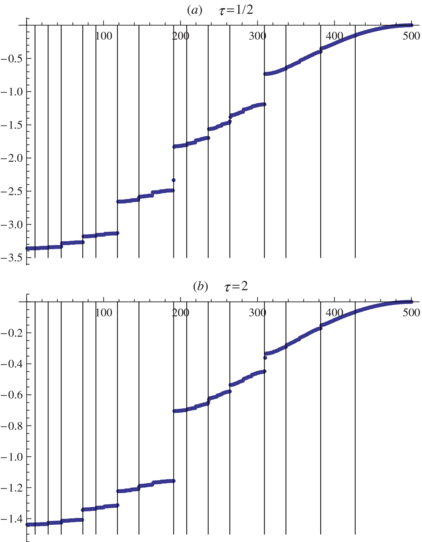
Figure 5. AbscissA: index i of the zeros xτ500, i, i = 1, ...500. Ordinate: zeros xτ500, i, i = 1, ..., 500. (a) τ = 1/2; (b) τ = 2. The vertical lines are at the hierarchical positions (see the text).
Download figure:
Standard image4.10. Numerical investigation of the orthogonality measure
The Gauss quadrature formula gives [17]  with p(x) a polynomial of degree at most 2n − 1, and the weigths Aτnk positive [17],

The prime in  means the derivative with respect to x of
  . The positive weights satisfy [17] ∑nk = 1An, kτ = 1. Let ψτn a bounded, right continuous, non-decreasing step function defined by [17]
Then [17] there is a subsequence of the sequence ψτn that converges to a distribution ψτ for which

for k = 0, 1, 2, ... . One says [17] that ψτ is a representative of  .
.
We shall now verify explicitly that for τ = 1, the sequence ψ1n converges and that dψ1 is indeed the measure of orthogonality for Chebyshev polynomials Uj. For the case τ = 1, ![$q_j^1(x)=U_j(1+x)=\frac{\sin [(j+1)\arccos (1+x)]}{\sin [\arccos (1+x)]}$](https://content.cld.iop.org/journals/1751-8121/44/42/425302/revision1/jpa392985ieqn94.gif) and (42) gives the zeros. Explicit computation from the last equality in (60) gives
and (42) gives the zeros. Explicit computation from the last equality in (60) gives ![$A_{n,k}^1=\frac{2}{n+1}\big(\sin \big[\frac{(n+1-k)\pi }{n+1}\big]\big)^2=\frac{2}{n+1}\big[1-\big(1+x_{n,k}^{1}\big)^2\big]$](https://content.cld.iop.org/journals/1751-8121/44/42/425302/revision1/jpa392985ieqn95.gif) . It is clear that the maximum jump of the step function ψ1n(x) is less than or equal to
. It is clear that the maximum jump of the step function ψ1n(x) is less than or equal to  and thus decreases to zero as n tends to infinity. The orthonormalization relation for Chebyshev polynomials reads
  . One therefore has to verify that in the limit n → ∞, A1n, k is equal to
  . Indeed,
 ![$x_{n,k+1}^1-x_{n,k}^1=2\sin \big[\frac{\pi }{2+2 n}\big]\sin \big[\frac{\pi -2 k \pi +2 n \pi }{2+2 n}\big]$](https://content.cld.iop.org/journals/1751-8121/44/42/425302/revision1/jpa392985ieqn99.gif)
![$\simeq \frac{\pi }{n+1}\sin \big[\frac{(n+1-k)\pi }{n+1}\big] =\frac{\pi }{n+1}\sqrt{1-\big(1+x_{n,k}^{1}\big){}^2}$](https://content.cld.iop.org/journals/1751-8121/44/42/425302/revision1/jpa392985ieqn100.gif) as n → ∞. To summarize, it has been verified explicitly that dψ1n(x) converges pointwise to
as n → ∞. To summarize, it has been verified explicitly that dψ1n(x) converges pointwise to  when n → ∞. Thus, the measure of orthogonality for τ = 1 has been deduced from the only knowledge of the zeros (42). The function whose derivative is
  and which takes the values 0 for x = −2 and 1 for x = 0 is

It is therefore natural to also investigate numerically the sequence ψτn for τ ≠ 1. Results are reported in figures 6(a) and (c). The fact that results for n = 100 (thin curve) appear as refinement of the results for n = 20 (thick gray curve) indicates that ψτn should indeed converge in some sense when n → ∞. However, in contrast with the case τ = 1, some discontinuities of the functions ψτn do not decrease as n increases, and one has evidence that ψτn converges toward a so-called devil staircase. The same numerical calculations made for τ = 1 give for n = 100 a step curve which almost coincides with (63) at the scale of the graph (see figure 6(b)). Figure 6 also indicates that the region where the ψτn are constant is clearly related to the gaps between the zeros, as should be the case from the defining relation (61). To conclude, the measure of orthogonality dψτ should involve, for τ ≠ 1, Dirac distributions whose supports are presently unknown functions of τ, and should exhibit self-similar structures.
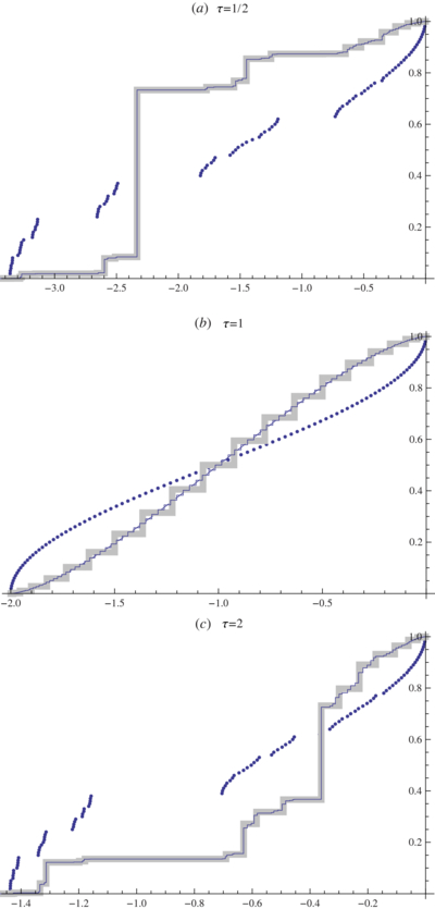
Figure 6. Thick gray line curve: graph of the function ψτ20(x) (61). Thin curve: graph of the function ψτ100(x) (61). Points: points of abscissa xτ100, i and of ordinate i/100, i = 1, ..., 100. (a) τ = 1/2; (b) τ = 1; (c) τ = 2. Part (b) also reports the continuous function (63), but it is almost indistinguishable from the discontinuous function ψτ100 at the scale of the graph.
Download figure:
Standard image5. Transmission coefficient at zero energy for critical points
We finally come back to the physical interpretation of critical points. When a target has a bound state near zero energy, it is generally expected that a resonance in the scattering process occurs at that energy.
5.1. Non-zero transmission coefficient of critical Fibonacci chains at zero energy
It will now be shown explicitly that the transmission coefficient throughout a Fibonacci chain in the limit of zero-energy incident plane wave is generically zero, except for a critical Fibonacci chain, i.e. a Fibonacci chain with the critical point.
It is well known [24] that the transmission coefficient t(k) for an incident plane wave with wave number k has the expression

with the second-order matrix Sn defined for a Fibonacci chain with n centers by


with di the intercenter distance (6). Now at the limit of zero energy,

From (64), it is clear that limk → 0t(k) = 0 for (Sn(0)21) ≠ 0. From the relations


one obtains
The left member has the same form as the one of recursion relations (12a). It can be verified by explicit computation that the whole factor in front of  in the right member of (72), i.e. M(d, 0) times the second-order matrices in the curly braces, is a matrix whose second line is 0, 0. Therefore, both (Sn(0)21) and (Sn(0)22) satisfy the recursion relation (12a). By explicit computation of S1(0) and S2(0) and comparison with (12b) and (13a), one deduces that

and therefore (Sτn(0)21) = 0 at critical Fibonacci chains. To summarize, the zero-energy transmission coefficient for a Fibonacci chain is zero except the cases of critical Fibonacci chains where it is
Let us further determine the matrix Sτn(0). From (12a) and (20a), one deduces that Qτn − Rn − 1τ satisfies the recursion relation (12a). By explicit calculation of Sτ1(0) and Sτ2(0) and from (12b) and (20b), one obtains (Sτn(0)22) = Qτn − 1 − Rn − 2τ. Now it is clear from (65), (67) and (66) that

Since

from (75), (76) and (73), one obtains

and, using (12a), (Sτn(0))11 = Qτn − 1 − Qn − 2τ. Finally, since  ,
,

with x defined by (9). The matrix element Sτn(0)12 can also be computed recursively with (75):
Equation (79) proves that Qτn − 1(x) divides (Qτn − 1(x) − Qn − 2τ(x))(Qτn − 1(x) − Rn − 2τ(x)) − 1. The transmission coefficient for the critical point i, i.e. for x equal to the zero xτn − 1, i (34) of Qτn − 1 will be denoted as tn, i(0). Then (74) can be expressed as

This proves that |Qτn − 2(xn − 1, iτ) + Rτn − 2(xn − 1, iτ)| ⩾ 2.
5.2. Complete transparency at zero energy of all critical Fibonacci chains when the number of centers is a Fibonacci number minus 1
The critical transmission coefficients (80) are not equal to zero but not necessarily equal to unity. For example, for n = 3,


and these transmission coefficients are equal to unity only for τ = 1. For the special cases where n is a Fibonacci number minus 1, and therefore the n − 1 intervals display palindromic property, it is now shown that all the critical transmission coefficients are equal to unity. (For spectral properties of infinite Fibonacci chains with palindromic properties, see [25].)
First note that  evaluated at the zeros of
  is equal to ±1. This property is obtained by taking the determinant of
  (19) at the zeros
  . Indeed this determinant is unity and equal to
  by (19) and (21). Then, from (21) and (80), one obtains

for all the Fk − 2 values of i.
Appendix A.
Fibonacci words or sequences and the golden ratio g have a long history and wide domains of applications. As a result, they are studied from different starting points in a huge number of publications in quite different fields. Reference [14] summarizes many results on Fibonacci sequences and related sequences, see also the text books [26, 27]. The purpose of this appendix is to obtain in a self-consistent way some properties useful for this work, assuming as starting point that (A.7) is a Fibonacci sequence. Throughout this appendix, α and β are positive irrational numbers satisfying (1/α) + (1/β) = 1, and  , the set of all positive integers 1, 2, ..., ∞, unless otherwise specified. In this appendix, the fractional part of x is denoted as {x}. One has x = ⌊x⌋ + {x}. The golden ratio satisfies the equivalent relations:

Another simple relation is

One way to obtain (A.2) is as follows: ⌊⌊kg⌋/g2⌋ = ⌊(k/g) − ({kg}/g2)⌋ = ⌊⌊k/g⌋ + {k/g} − ({kg}/g2)⌋. Now  . Therefore,
  .
.
The so-called Beatty theorem [28, 29] states then that the two sets  and
and  are disjoint and their union is the set
  , and therefore the two sets
  and
and  form a partition of
  . For the sake of generality, further results are now considered in terms of α and β, but the case of interest in this paper is α = g and β = g2.
Let  . Since (1/α) + (1/β) = 1, n = (n/α) + (n/β) = ⌊n/α⌋ + ⌊n/β⌋ + {n/α} + {n/β}. Since {n/α} + {n/β} < 2, one has {n/α} + {n/β} = 1 and n = ⌊n/α⌋ + ⌊n/β⌋ + 1. Therefore, every
  can be written as a sum of two different integers in the following way:

Another useful relation is

Note that the two arguments of the minimum function min are different by the Beatty theorem. To prove (A.4), note that  and the same relations with β in place of α. Therefore, the two arguments of min in (A.4) are greater than or equal to n. Let us first show that
  is impossible for α irrational. Indeed, dividing by α and subtracting
  from both members,
  , and therefore
  which contradicts the fact that α is irrational. Then first suppose that
  . Then
  and (A.4) is satisfied. Suppose now the opposite case, i.e.
  . If we then show that
  cannot be greater than or equal to 1, (A.4) is proved. The simultaneous inequalities
  and
and  are indeed impossible, because dividing the first by α, the second by β, and summing, one obtains
  . In this paper, (A.4) will be used as followed: every positive integer satisfies one and only one of the following two equations:


Our starting point is that the sequence uk, k = 1, 2, ...,


is a Fibonacci sequence 10110⋅⋅⋅ as defined by the substitution s (1a), (1b) with 1 for A and 0 for B. (A.8) can be obtained from (A.7) using g = 1 + 1/g. (A.9) can be obtained from (A.8) using (A.3). In (A.10), (A.11) and (A.12), χ[a, b) is the characteristic function over the interval [a, b), a included, b excluded. (A.10) can be obtained by noting that if uk = 1, then (A.7) gives ⌊⌊kg⌋ + {kg} + g⌋ = ⌊kg⌋ + 2 and therefore  . (A.11) can be obtained by noting that if uk = 1, then (A.8) gives
  and therefore {k/g} + 1/g ⩾ 1. (A.12) can be obtained by noting that if uk = 1, then (A.9) gives
  and therefore
  .
.
If we sum both members of (A.8) from k = 1 to k = n, one obtains the number of 1 for the left member and  for the right member. Performing the same calculation with (A.7) and (A.9), the number nA of A in a Fibonacci word ABAA⋅⋅⋅ of n letters can be expressed as

and, using (A.3), the number nB of B is

From these results follows that in the limit n → ∞, the proportion of A is 1/g and the proportion of B is 1/g2. The relation  shows that for
  ,
,  . Suppose now uk = 1. Then (A.8) gives
  . Thus, if uk = 1, then
  . On then deduces from (A.13) that if the letters of a Fibonacci chain are numbered from left to right starting with 1, for example, 1, 2, 3, 4, 5 for ABAAB, then the kth A has position ⌊kg⌋. Then, by the Beatty theorem the kth B has position ⌊kg2⌋. Thus, for
  ,
,


From (A.7) and (A.13), it is clear that the difference of position of two successive A can only be 1 or 2 and therefore BB never occurs in a Fibonacci word. From (A.7) and (A.14), and from g2 = g + 1, it is clear that the difference of position of two successive B can only be 2 or 3 and therefore AAA never occurs in a Fibonacci word. From (A.7) and (A.13), the difference of position between the (k + 1)th A and the kth A is 1 + uk. But it is also 2 if u1 + ⌊kg⌋ = 0 and 1 if u1 + ⌊kg⌋ = 1. Therefore,

In a Fibonacci word of n letters, (A.13) shows that the last letter is A if  . In that case, (A.8) shows that the condition can also be written as
  , nA (A.13) is also equal to
  and nB (A.14) is then also equal to
  . In a Fibonacci word of n letters, (A.14) shows that the last letter is B if
  . In that case, (A.5) is not satisfied because the last letter is not A, and therefore (A.6) is satisfied. In that case, nB (A.14) is also equal to
  , and nA (A.13) is also equal to
  .
.
In a Fibonacci word of n letters, the position of the last B,  , is of course smaller than or equal to n. Then, one deduces that the largest integer k such that ⌊kg2⌋ ⩽ n is
  .
.
In a Fibonacci word of n letters, the position of the last A,  , is of course smaller than or equal to n. Then, one deduces that the largest integer k such that ⌊kg⌋ ⩽ n is
  .
.
From the two previous results, one deduces that the largest integer k such that ⌊⌊kg2⌋g⌋ ⩽ n is  .
.
If, in a Fibonacci word, A is replaced by AA, for example, the step 4, ABAAB gives AABAAAAB, then the kth B has the position ⌊⌊kg2⌋g⌋. Indeed, consider a Fibonacci word with k B and ending with B. The position of this last B is ⌊kg2⌋. Under the replacement A → AA, the number of A,  , is doubled so that the position of the last B becomes
  , and using 1/g = g − 1, one obtains ⌊⌊kg2⌋g⌋.
Let us consider the sequence sk = (uk − 1 + uk) starting with k = 2. sk can take only the values 1 and 2 since uk can take only the values 0 and 1 and since uk and uk − 1 cannot be simultaneously equal to 0. We are looking for the positions of 2 in the sequence s2, s3, ... . The condition sk = 2 requires first that uk = 1, i.e. k must be of the form ⌊ℓg⌋. We then have s⌊ℓg⌋ = 2 if and only if the (ℓ − 1)th 1 has position ⌊ℓg⌋ − 1, i.e. if and only if ⌊(ℓ − 1)g⌋ = ⌊ℓg⌋ − 1 which implies according to (A.7) that uℓ − 1 = 0, i.e. ℓ − 1 = ⌊mg2⌋. Thus, sk = 2 if and only if k = ⌊(⌊mg2⌋ + 1)g⌋. (A.16) gives ⌊(⌊mg2⌋ + 1)g⌋ = ⌊⌊mg2⌋g⌋ + 1. Therefore, the sequence s2, s3, ... is the sequence obtained from a Fibonacci sequence with A = 1, B = 2, by replacing all 1 by the juxtaposition 11. The definition 1 gives s2, s3, ..., sn + 1 = Wn(11, 2).
Let us now calculate
Let us now calculate the number n1 of 1 and the number n2 of 2 in the n terms sequence s2, s3, ..., sn + 1:
Since n = n1 + n2, one obtains

Before proceeding further, let us prove that
(A.3) gives  . Consider first the case un = 1. Then (A.8) shows that (A.21) is equivalent to
  . (A.9) gives
  . Now
. Now  . (A.11) gives
  . Thus, (A.21) is proved for the case un = 1. Consider now the case un = 0. Then un − 1 = 1 (since two consecutive 0 cannot appear in the sequence uk), and if we replace n by n − 1 in (A.21), one obtains a valid equation. Subtracting this equation from (A.21), one obtains using (A.8) un − 1 for the difference of the left members, and using (A.9 )
  for the difference of the right members. Since un − 1 = 1 = 1 − un, it remains therefore to prove
  . This is valid since using (A.8),
  . Thus, (A.21) is proved and allows us to write (A.20) as
It is clear from the definition sk = uk − 1 + uk that the number n2 of 2 in the n-term sequence s2, s3, ..., sn + 1 is also the number of consecutive AA in a Fibonacci word (Wn + 1(A, B)). Thus, the number nAA of consecutive AA in a Fibonacci word (Wn(A, B)) is
The number  of isolated A in a Fibonacci word of n letters can then be deduced:
so that finally
For the last equality, note that  .
.
Appendix B.
This appendix proves that the Fibonacci words of length Fk − 2 are palindromes by the substitution method. (For a proof based on the concatenation method, see [20].)
Intermediate results are now first considered. Let wn be an arbitrary word of n letters in the alphabet A, B (not necessarily a Fibonacci word). For example, w4 = BABB. The word with zero letter will be denoted as ∅. The operator which drops the first letter of a word is denoted as ℓ. For example, ℓ(AABB = ABB). When each letter of a word wn is replaced according to the substitution rules (1a) and (1b), the resulting word is denoted as s(wn). We then have

The proof is immediate since the first letter of s(wn) is always A due to (1a) and (1b). Let the overline denote the operation of reversing the order of all the letters of a word. For example,  . Of course, we have
  and
and  . An important property is

i.e. the reversing operator commutes with the operator ℓ ∘ s. Introducing the operator d which drops the last letter of a word, and replacing wn by  , (B.2) can be written as

Note that s(w) and  have the same number of letters. We shall prove (B.2) by induction, and note first that it is true for n = 1. Indeed for w1 = A, the left-hand side (lhs) of (B.2) gives
  and the right-hand side (rhs) of (B.2) gives
  . Now for w1 = B, the lhs of (B.2) gives
  and the rhs of (B.2) gives
  . Therefore, (B.2) is true for n = 1. Suppose it is true for n. An arbitrary word wn + 1 can be obtained from a word wn as wnA or wnB. First consider wnA. The lhs of (B.2) gives
  . The last equality follows from (B.1). The rhs of (B.2) gives
  . We therefore have to compare
  with
with  . They are equal since property (B.2) is assumed to be true for every wn. It remains to consider wnB. The lhs of (B.2) gives
  . The last equality follows from (B.1). The rhs of (B.2) gives
  . We therefore have to compare
  with
with  . They are equal since property (B.2) is assumed to be true for every wn. Thus, (B.2) is proved.
We are now ready to prove the palindromic property. We proceed by induction and first note by inspection that the property is true for k = 3, 4, 5. Next we note that the last two letters of  are alternatively AB or BA as j increases. This is immediate since
  and then (1a) and (1b) give the result. Suppose the palindromic property is true for k. Then

with u a word, x either ∅ (when Fk even) or A or B (when Fk odd), and y either AB or BA. We extend (1a), (1b) by s(∅) = ∅:

Since s(AB) = ABA and s(BA) = AAB,

We therefore have to prove that the word

has mirror symmetry by reflection through a plane perpendicular to it and cutting it in its middle. (The equality in (B.7) is due to (B.3).)
Suppose that Fk is even (i.e. k is divisible by 3). Then x = ∅ and the word with an odd number of letters  has the required mirror symmetry.
Suppose that Fk is odd and x = B. Then s(x) = A and the word  has an even number of letters. The required mirror symmetry is obtained if the first letter of
  is A. This is the case according to (1a) and (1b).
Suppose finally that Fk is odd and x = A. Then s(x) = AB and the word with an odd number of letters  has for mirror symmetry plane the plane cutting B since the first letter of
  is A according to (1a) and (1b).