

Abstract
Considering the significant role of global methane emissions in the Earth's radiative budget, global or regionally persistent increasing trends in its emission are of great concern. Understanding the regional contributions of various emissions sectors to the growth rate thus has policy relevance. We used a high-resolution global methane inverse model to independently optimize sectoral emissions using GOSAT and ground-based observations for 2009–2020. Annual emission trends were calculated for top-emitting countries, and the sectoral contributions to the total anthropogenic trend were studied. Global total posterior emissions show a growth rate of 2.6 Tg yr−2 (p < 0.05), with significant contributions from waste (1.1 Tg yr−2) and agriculture (0.9 Tg yr−2). Country-level aggregated sectoral emissions showed statistically significant (p < 0.1) trends in total posterior emissions for China (0.56 Tg yr−2), India (0.22 Tg yr−2), United States (0.65 Tg yr−2), Pakistan (0.22 Tg yr−2) and Indonesia (0.28 Tg yr−2) among the top methane emitters. Emission sectors contributing to the above country-level emission trend are, China (waste 0.35; oil and gas 0.07 Tg yr−2), India (agriculture 0.09; waste 0.11 Tg yr−2), United States (oil and gas 1.0; agriculture 0.07; coal −0.15 Tg yr−2), Brazil (waste 0.09; agriculture 0.08 Tg yr−2), Russia (waste 0.04; biomass burning 0.15; coal 0.11; oil and gas −0.42 Tg yr−2), Indonesia (coal 0.28 Tg yr−2), Canada (oil and gas 0.08 Tg yr−2), Pakistan (agriculture 0.15; waste 0.03 Tg yr−2) and Mexico (waste 0.04 Tg yr−2). Additionally, our analysis showed that methane emissions from wetlands in Russia (0.24 Tg yr−2) and central African countries such as Congo (0.09 Tg yr−2), etc. have a positive trend with a considerably large increase after 2017, whereas Bolivia (−0.09 Tg yr−2) have a declining trend. Our results reveal some key emission sectors to be targeted on a national level for designing methane emission mitigation efforts.
Export citation and abstract BibTeX RIS

Original content from this work may be used under the terms of the Creative Commons Attribution 4.0 license. Any further distribution of this work must maintain attribution to the author(s) and the title of the work, journal citation and DOI.
Corrections were made to this article on 28 March 2024. The Author affiliations were amended.
1. Introduction
Methane (CH4) is a greenhouse gas, second to carbon dioxide (CO2) in its abundance in the Earth's atmosphere. Its capacity to trap heat in the atmosphere by absorbing radiation is 25 times larger than that of carbon dioxide. The atmospheric concentration of methane has more than doubled during the last two centuries due to industrialization (720 to1920 ppb from 1750 through 2023). Owing to the more significant warming potential and the shorter lifetime in the atmosphere compared to CO2, a significant short-term effect on global warming is expected by deliberate actions to reduce methane emissions from anthropogenic sources. Methane is emitted from various sources, which are either anthropogenic or natural. The anthropogenic sources include coal mines, oil and gas infrastructures, landfills, agriculture, etc. The countries that are primary sources of anthropogenic methane are China, the United States, Russia, India, Brazil, Nigeria, and Mexico, which altogether emit almost half of the anthropogenic methane emissions (Crippa et al 2020). Among them, the countries from Asia contribute a significant proportion to the current growth rate in line with the economic development of this region (Wang et al 2021).
Understanding the temporal changes in atmospheric methane emissions is essential, but the drivers of these changes over recent decades remain poorly understood. The growth rate in atmospheric CH4 slowed in the early 1990s, followed by a stabilization period during 2000–2006. Since 2007, global atmospheric CH4 concentrations have begun to rise again. In the latest year in this study, 2020, methane was reported to have an unusual increase in the atmosphere (e.g. Lan et al 2022, Qu et al 2022). Several recent studies have arrived at contrasting conclusions about the causes of these changes post-2007, citing increasing emissions of CH4 from fossil fuels, agriculture, wetlands, or decreased hydroxyl radicals (O.H.) (e.g. Hausmann et al 2016, Nisbet et al 2016, Rigby et al 2017) as main drivers due to different measurements, methodologies, and periods considered. Such discrepancies highlight the need to reconcile our understanding of the drivers of the growth in atmospheric CH4 to design mitigation policies (Zhang et al 2022). Capabilities to assess sectoral trends of these emissions using top–down approaches will help understand the geographical and sectoral origins leading to the overall increase in atmospheric methane. Therefore, attempts to study such spatiotemporal variability using flux inverse models are very useful. Recent developments in greenhouse gas observations from space have opened unprecedented capacities for independent agencies to monitor emissions over regions of interest. Widely used space-based observations include those with the Greenhouse Gases Observing Satellite, GOSAT (Kuze et al 2009, Yokota et al 2009), and the Tropospheric Monitoring Instrument onboard Sentinel-5P satellite (Veefkind et al 2012). Though national governments report sector-wise emissions of various greenhouse gases, the estimates on which the reports are based are probably dependent on inaccurate or incomplete data from multiple sub-national agencies, which have varying levels of scrutiny in various steps of the compilation of the data. When aggregated to the national level, these bottom–up inventories can be flawed due to the above reasons, such as incomplete accounting of the activities, errors in emission factors, etc. In this case, a comparison with nationally prepared inventories with top–down flux estimates becomes very important. In these top–down emission estimates based on an inversion of atmospheric observation of greenhouse gas concentrations, satellite observations play a quite useful role in augmenting ground-based observations in regions where they are sparse.
Recent studies have analyzed country-level methane budgets from individual inversions or ensemble of inversions from various inverse models (e.g. Deng et al 2022, Worden et al 2022) and conducted a comprehensive analysis of the sectoral budget and its comparison to national inventories. Beyond a country-level estimate, in this study we aim to provide the country-level sectoral methane emissions trends, for the large emitting countries, that have contributed to their total emission growth in the past decade. Here we use the total column mixing ratio of methane from the GOSAT satellite and information from ground-based sources to infer sectoral emissions using an inverse model. The simulations were primarily carried out for the GCP global methane budget (GMB) inversion intercomparisons for the update of the latest GMB reported in 2020 (Saunois et al 2020). Posterior emissions were estimated for five anthropogenic sectors- agriculture, waste, biomass burning, coal, oil and gas, and one natural sector, wetlands, for 2009–2020. The biomass burning sector discussed here includes biofuels as well, but for brevity, we refer to the sector as biomass burning in the entire paper. The trends for each sector were analyzed on a 1° × 1° grid and aggregated to annual country totals.
2. Data and methods
2.1. Methane prior fluxes and uncertainties
We used the emissions database for Global Atmospheric Research (EDGAR v6) as a primary database for prior anthropogenic methane emissions (Crippa et al 2020). The emission sectors in the EDGAR database include biofuels, coal, livestock, rice, and waste sources. We used emissions from the oil and gas sector by the greenhouse gas and air pollution interactions and synergies model (Höglund-Isaksson 2012). Emissions from biomass burning were taken from the Global Fire Emission Database, GFED v4.1 (Randerson et al 2017), and emissions from wetland and termite sources were from Saunois et al (2020). Other minor emission sources from the ocean were taken from Weber et al (2019) and geological sources from Etiope et al (2019). Methane sink in the soil was taken from Murguia-Flores et al (2018). All these fluxes were provided to the model at 0.1° × 0.1° latitude–longitude resolution and monthly time steps. Of the above emissions, monthly climatology was used for geological, ocean, termites, and wetland sources. A mean picture of all the groups of prior emission sectors is given in figure 1.

Figure 1. Mean (2009–2020) prior sectoral methane fluxes used in this study (gCH4 m−2 yr−1) for (a) agriculture, (b) waste, (c) biomass burning, (d) coal, (e) oil and gas, and (f) wetlands sectors.
Download figure:
Standard image High-resolution imageThe prior uncertainties for each of the six sectors (agriculture, waste, biomass burning, coal, oil and gas, wetlands) were provided based on their respective climatological fields. For anthropogenic sectors, 30% of their respective monthly varying climatologies were prescribed, while 50% was set for wetland prior.
2.2. Observations
For inversion, we have used a set of observations consisting of ground-based and remote sensing data. The following sections describe the details of how these observations were used in the inversion and how the uncertainties were calculated.
2.2.1. Surface observations
We used weekly or continuous atmospheric CH4 observations from a global network of surface stations, aircraft, and ship tracks. This mainly consists of Obspack (GLOBALVIEWplus_v4.0_2021-10-14, Schuldt et al 2021) observations, with additional observations from the ICOS network (ICOS RI 2021). For continuous measurements, we used observations during well-mixed atmospheric conditions (14:00–16:00 local time) averaged to daily values to improve the representativeness. For high-altitude sites, 04:00–06:00 local time was used to avoid the effects of upslope transport of local emissions due to daytime heating. For the observations from surface sites, data uncertainties were defined based on the root mean squared error (RMSE) with its prior forward simulations. A minimum uncertainty value of 6 ppb was set to allow more freedom for the inversion in the Southern Hemisphere. The rejection criteria for the surface, aircraft, and ship observations were decided based on the variance in the data. The site-specific details of the observation data are tabulated in table S1.
2.2.2. Greenhouse gas observing satellite (GOSAT) observations
The Greenhouse gases observing satellite (GOSAT; Kuze et al 2009, Yokota et al 2009) is a sun-synchronous satellite observing column-averaged dry-air mole fractions of methane and carbon dioxide in the shortwave infrared band with observations made around 13:00 local time. It has a surface observation footprint diameter of about 10 km and has a three-day repeat cycle in normal observation mode. In this study, we used XCH4 retrieved from the GOSAT at the National Institute for Environmental Studies, Japan (NIES Level 2 product, v.02.95; Yoshida et al 2013) for 2009–2020 to constrain methane emissions. The bias of this version of GOSAT XCH4 products is empirically corrected using ground-based data. Data uncertainty for the GOSAT retrievals was set to 60 ppb, with a rejection threshold of 30 ppb. Such a large data uncertainty was applied to the GOSAT retrievals because the volume of GOSAT observations was much larger than that of ground-based observations. A smaller uncertainty could result in an overfit to the GOSAT data, although measurement precision is higher for the ground-based observations.
A spatial map of the observation location used in this study is given in figure 2. A list of stations and the details, such as respective references, are given in supplementary table S1. For an independent validation, we used aircraft observations that were not assimilated in the inversion (figure S4).
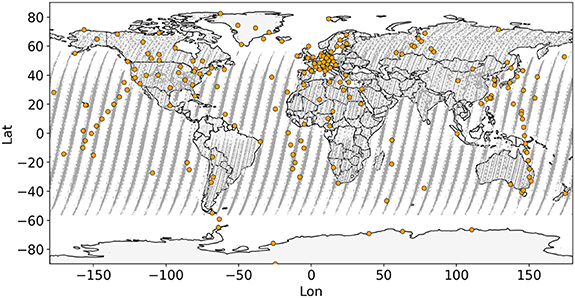
Figure 2. The locations of methane observations used in this study include surface, ship, aircraft (orange), and GOSAT (grey) observations for 2009–2020.
Download figure:
Standard image High-resolution image2.3. NTFVAR inverse modeling system
In this study, we have used a global Eulerian–Lagrangian coupled model NIES-TM–FLEXPART-variational model (NTFVAR) that consists of the NIES model as the Eulerian three-dimensional transport model and the FLEXPART (FLEXible PARTicle dispersion model) as the Lagrangian particle dispersion model. This study used a variational inversion scheme to the high-resolution variant of the NIES-TM–FLEXPART transport model and its adjoint presented by Maksyutov et al (2021). The Lagrangian model calculates the local influence of fluxes on the observations, while the Eulerian model provides the slowly varying background concentrations. For the Lagrangian model, virtual particles were released from each observation point and transported two days backward in time with the three-dimensional wind field with parameterizations for turbulence and convection. We used the GOSAT averaging kernel sensitivities to distribute vertically the total particles. The time integral of particle density below the mixing height in the flux grid gives the surface flux sensitivity of the trace gas mixing ratio at the receptor (Ganshin et al 2012). The methane mixing ratio at the observation location is then obtained as the area integral of the emission sensitivity multiplied by the respective flux (Lin et al 2003, Ganshin et al 2012). The model samples the background concentrations from the Eulerian model at the time of termination of Lagrangian Particles (coupling time, approximately two days before observation time) and adds to the concentration at the observation point calculated by the Lagrangian model due to local fluxes. More details on the implementation of the coupled model are described by Ganshin et al (2012) and Belikov et al (2016). The advantages of this coupled system in simulating continental observations were demonstrated by Ganshin et al (2012). While the Global Eulerian model represents the large-scale variability in the observation, the Lagrangian part efficiently represents the fine-scale variability in the observation due to local fluxes. The details of the inverse model development can be found in Maksyutov et al (2021). The Eulerian model NIES-TM with a horizontal resolution of 3.75° × 3.75° and 42 hybrid-pressure levels is driven by ERA5 reanalysis winds and is based on a revised model version used in Maksyutov et al (2021). The tracer advection scheme was revised to implement the transport of first-order moments (Van Leer 1977, Russell and Lerner 1981) for advection, which leads to better reproducing sharp concentration gradients. Due to the availability of vertical velocity in the native model coordinates, the ERA5 winds allow for a more accurate reconstruction of grid-scale mass balance. As a result, the modified model fixes the weak interhemispheric SF6 gradient visible in the intercomparison by Krol et al (2018) made with the former model version by Belikov et al (2013). Lagrangian model FLEXPART v.8.0 was run in backward mode with a surface flux resolution of 0.1°× 0.1°, driven by the meteorological fields from the Japanese Meteorological Agency (JMA) Climate Data Assimilation System (JRA-55/JCDAS; Onogi et al 2007, Kobayashi et al 2015).
The optimization was applied to a time window of 18 months for each optimized year, and the simulation started on 1 October, three months ahead of the target year. A spin-up period of 3 months is given to let the inversion adjust the modeled concentration to the observations so that a balance is achieved between fluxes, concentrations, and concentration trends. The inverse modeling problem is formulated and solved to find the optimal value of corrections to prior fluxes considering mismatches of observations and modeled concentrations. Variational optimization is used to obtain flux corrections implemented by multiplying monthly varying prior flux uncertainty fields at a 0.1° × 0.1° resolution by five anthropogenic (agriculture, waste, coal, oil and gas, and biomass burning) and wetland scaling factors at a half-monthly time step. We assume that the strong emission sources are not collocated, and a large number of observations capture different mix of source categories, which allows the model to put weights to different sectors separately. The inverse model internally optimizes scaling factor fields for each flux category at the resolution of 0.2°× 0.2° and applies spatial flux covariance length of 500 km and temporal correlation distance of 15 d. We optimized fluxes for 12 yr from 2009 to 2020. A more detailed description can be found in Maksyutov et al (2021).
The inverted fluxes were remapped to 1° resolution for trend analysis. These were further aggregated using country masks for analysis at the country level. The trend analysis was carried out using the Mann–Kendall statistical test (Mann 1945, Kendall 1975) following pre-whitening of the data proposed by Yue and Wang (2002) to avoid the influence of serial correlation.
3. Results
3.1. Posterior fluxes
The sector-wise flux corrections optimized by the inverse model averaged for the 2009–2020 period, are given in figure 3. This flux adjustment for each sector added to the respective prior gives the posterior emissions, and a global perspective of the sectoral posterior fluxes is discussed below. We have used monthly fluxes of anthropogenic and natural methane sources in this study and optimized fluxes in six categories. On average, our prior global total emissions were 592 Tg yr−1 and the posterior estimate 583 Tg yr−1 compared to 572 Tg, for example, by Stavert et al (2021) or 576 Tg by Saunois et al (2020) On a sector level, our flux corrections by the model indicate that for the agriculture sector, the emissions over Southern South America, India, Australia, parts of China, Europe, and Russia are over-estimated by the prior inventory (EDAGAR v6), where the model adjusted the prior emissions downward. The largest reduction found was for central eastern parts of South America, including parts of Brazil and Argentina, the Indian subcontinent, and southeastern parts of China and eastern Europe. However, there is an upward revision by the model over the northern parts of South America, including Brazil and Colombia, the central-eastern African region, including Ethiopia, Kenya, and Tanzania, southeast Asian countries, eastern China, Japan, and western Europe. Flux adjustments for the waste sector were overall positive for northern parts of South America, central African countries, and Southeast Asian countries, whereas Europe, the Middle East, India, and China have lower emissions than the prior. Emissions from biomass burning had strong negative corrections to the prior over India, China—especially eastern provinces, and parts of Europe, whereas large-scale upward corrections were found over Russia, Canada, and Australia. Posterior emissions for the coal sector from China suggested a southward shift in the emission location and an overall reduction over Australia, India, the United States, and parts of Europe, with pockets of positive corrections and an apparent increase over southeast Asian countries and Russia. The model suggested an underestimation in the oil and gas sector over the United States, Canada, India, and China and some overestimation over Russia and the Middle East countries.
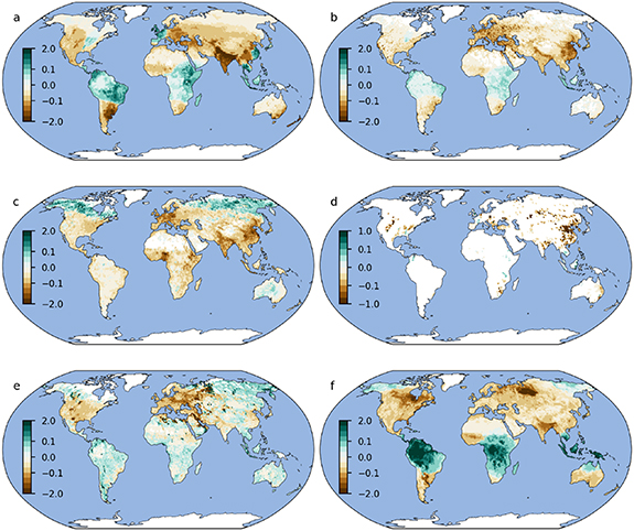
Figure 3. Sectoral correction to prior fluxes (gCH4 m−2 yr−1) for (a) agriculture, (b) waste, (c) biomass burning, (d) coal, (e) oil and gas, and (f) wetlands sectors estimated by the inverse model.
Download figure:
Standard image High-resolution imageThe prior wetland emissions aggregated for the globe were 151.2 Tg yr−1, and the posterior estimate was 160 Tg yr−1. Our posterior wetland emissions indicate that the prior emissions were overestimated in Siberia, Canada, southern South America, India, and Southeast Asia. On the contrary, the model corrects the wetland emissions upward in tropical South America and southern parts of North America. Towards the end of the analysis period, our inversion revealed a substantial increase in methane emissions for certain African countries, which was reported by recent studies such as Qu et al (2022). Details of which are discussed in the next section. A comparison of observations, prior forward simulations, and simulations with optimized fluxes for selected sites are given in figure 4, and the rest of the observations are given in supplementary figure S5.
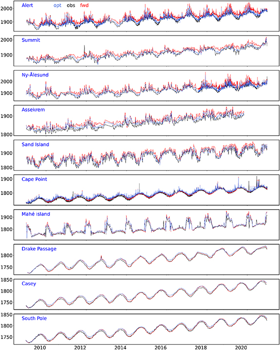
Figure 4. Time series of observation, prior and optimized forward simulations for selected sites. Sites were chosen to represent high-latitude and low-latitude in both hemispheres.
Download figure:
Standard image High-resolution imageWe conducted a validation simulation using independent surface (observations mentioned in 2. 2. 1, that were not assimilated in the inversion step) and aircraft (CARIBIC) observations, where RMSE for prior and optimized forward simulations were analyzed (figure 5). As these datasets were not used in the inversion, they provide an independent validation of the optimized fluxes. Figure 5 presents the percentage RMSE reduction for both surface and aircraft observations on a 2° grid. Overall, optimization reduces the prior bias and RMSE with some exceptions for surface sites as well as some levels of aircraft data. The inset figure in figure 5 shows the 500 m averaged prior and posterior RMSE for aircraft data. A general trend of weak RMSE reduction can be seen over regions having fewer surface observation sites, especially over Asia, compared to regions with dense observation networks.
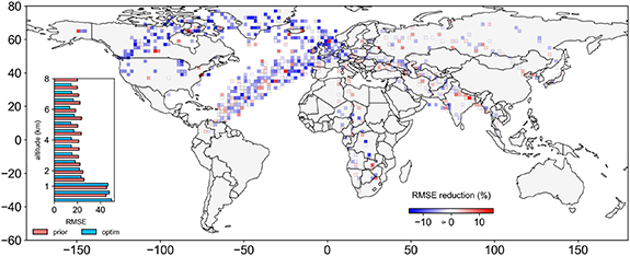
Figure 5. Validation of inversion using independent observations. The colored grid cells present the global map of RMSE reduction (in percentage, aggregated onto 2° grids) resulting from optimization for surface and aircraft observations not used in the inversion. The inset plot shows the vertical profile of 500 m averaged RMSE for aircraft observations (provided by the European research infrastructure IAGOS-CARIBIC) in the prior and optimized forward simulations.
Download figure:
Standard image High-resolution image3.2. Country total sectoral emissions and uncertainties for large emitters
We estimated the total sectoral emissions and their uncertainties for the top emitting countries (table 1). The figures mentioned here are in Tg yr−1 averaged for the whole study period. In the agricultural sector, China (21.49 ± 1.47), India (16.30 ± 1.89), Brazil (15.49 ± 0.39), USA (8.8 ± 0.27) and Pakistan (4.77 ± 0.38) are some of the largest emitters. Zhang et al (2022) reported around 22 Tg for the 2010–2017 period from rice and livestock in China, which is consistent with our results. The biennial update report (BUR3) of the government of India reports 14.4 Tg methane for 2016 from agriculture, against our estimate of 19 Tg (BUR3, MoEFCC 2021). A potential reason for lower values in the national inventory could be lower emissions from the livestock sector due to Tier 1 method and emission factors of 2006 IPCC guidelines (IPCC 2006) (Deng et al 2022). BUR of Brazil indicates the emission from the agricultural sector for 2015 was around 12.3 Tg (70% of total anthropogenic), while our estimate for 2015 was 15 Tg. Our anthropogenic posterior estimate for Brazil (21.23 Tg) is comparable to other studies, for example, Tunnicliffe et al (2020) (19 Tg), but differs in magnitude with some others (e.g. Worden et al 2022; 30.6 Tg). A similar underestimation in national greenhouse gas inventory was reported by Deng et al (2022) for the agriculture and waste sector collectively using GOSAT inversions. Major contributors to the waste sector emissions are China (12.43 ± 0.66), India (6.06 ± 0.15), Brazil (4.64 ± 0.08) and USA (4.22 ± 0.06). According to India BUR3, the total emissions from the waste sector for 2016 is 2.82 Tg as opposed to our estimated value of 6.5 Tg.
Table 1. Country-level estimates of sectoral emissions and their uncertainties (Tg yr−1) averaged for 2009–2020.
| Country | Agri. | Waste | Biom.Biof. | Coal | Oil&Gas | Wetland |
|---|---|---|---|---|---|---|
| Argentina | 2.77 ± 0.37 | 0.51 ± 0.01 | 0.09 ± 0.00 | 0.00 ± 0.00 | 0.81 ± 0.01 | 4.26 ± 0.18 |
| Australia | 2.15 ± 0.32 | 0.32 ± 0.01 | 0.51 ± 0.01 | 0.99 ± 0.07 | 0.22 ± 0.00 | 4.24 ± 0.18 |
| Bolivia | 0.77 ± 0.02 | 0.07 ± 0.00 | 0.31 ± 0.00 | 0.18 ± 0.00 | 5.33 ± 0.31 | |
| Brazil | 15.49 ± 0.39 | 4.64 ± 0.08 | 1.47 ± 0.03 | 0.05 ± 0.00 | 0.31 ± 0.01 | 33.38 ± 1.83 |
| Canada | 1.01 ± 0.02 | 0.55 ± 0.01 | 0.95 ± 0.01 | 0.08 ± 0.01 | 2.48 ± 0.10 | 10.49 ± 0.65 |
| China | 21.49 ± 1.47 | 12.43 ± 0.66 | 2.39 ± 0.02 | 16.63 ± 0.86 | 2.47 ± 0.02 | 2.98 ± 0.09 |
| Colombia | 1.83 ± 0.05 | 0.78 ± 0.01 | 0.06 ± 0.00 | 0.20 ± 0.00 | 0.51 ± 0.02 | 6.65 ± 0.38 |
| Rep. of Congo | 0.02 ± 0.00 | 0.02 ± 0.00 | 0.08 ± 0.00 | 0.06 ± 0.00 | 5.83 ± 0.25 | |
| Demo. Rep. of Congo | 0.25 ± 0.00 | 0.54 ± 0.02 | 1.31 ± 0.04 | 0.02 ± 0.00 | 13.46 ± 0.79 | |
| India | 16.30 ± 1.89 | 6.06 ± 0.15 | 1.24 ± 0.05 | 1.38 ± 0.06 | 0.45 ± 0.01 | 3.81 ± 0.16 |
| Indonesia | 3.58 ± 0.32 | 1.88 ± 0.10 | 2.13 ± 0.01 | 3.71 ± 0.23 | 0.94 ± 0.07 | 14.00 ± 0.89 |
| Iraq | 0.14 ± 0.03 | 0.38 ± 0.01 | 0.00 ± 0.00 | 6.00 ± 0.90 | 0.09 ± 0.00 | |
| Mexico | 2.49 ± 0.05 | 2.24 ± 0.03 | 0.19 ± 0.00 | 0.02 ± 0.01 | 0.30 ± 0.02 | 1.34 ± 0.05 |
| Nigeria | 1.62 ± 0.04 | 1.25 ± 0.02 | 0.78 ± 0.01 | 0.00 ± 0.00 | 2.13 ± 0.38 | 1.70 ± 0.11 |
| Pakistan | 4.77 ± 0.38 | 1.15 ± 0.03 | 0.30 ± 0.00 | 0.03 ± 0.00 | 0.50 ± 0.03 | 0.15 ± 0.01 |
| Peru | 0.54 ± 0.00 | 0.25 ± 0.00 | 0.04 ± 0.00 | 0.00 ± 0.00 | 0.05 ± 0.00 | 8.54 ± 0.57 |
| Russia | 1.52 ± 0.02 | 3.02 ± 0.04 | 1.90 ± 0.23 | 2.34 ± 0.10 | 19.83 ± 0.52 | 10.52 ± 0.86 |
| Sudan | 2.48 ± 0.03 | 0.39 ± 0.01 | 0.41 ± 0.00 | 0.00±-0.00 | 1.20 ± 0.03 | 3.10 ± 0.23 |
| Thailand | 2.76 ± 0.51 | 0.86 ± 0.03 | 0.12 ± 0.03 | 0.01 ± 0.00 | 0.13 ± 0.01 | 1.17 ± 0.08 |
| USA | 8.80 ± 0.27 | 4.22 ± 0.06 | 0.48 ± 0.06 | 2.02 ± 0.39 | 14.10 ± 0.19 | 5.43 ± 0.28 |
| Venezuela | 1.15 ± 0.02 | 0.37 ± 0.00 | 0.09 ± 0.00 | 0.01 ± 0.00 | 1.51 ± 0.03 | 4.81 ± 0.37 |
Emissions from the oil and gas sector are significant for Russia and the USA, with 19.8 ± 0.5 and 14.1 ± 0.19 Tg, respectively, both are higher than the national inventories and on the upper side of the range of previous GOSAT inversions (e.g. Deng et al 2022). For the United States, this figure is consistent with studies such as Lu et al (2023; GOSAT inversion; 14.8 Tg) or Alvarez et al (2018) where they report mean CONUS emission of 13 Tg for 2015, obtained from field measurements upscaled to national totals (not by inversion).
We further compared our inverse model estimates of 2018 for India to an independent bottom-up emission inventory developed for India's anthropogenic and wetland sectors at a high resolution of 0.1° (Sahu et al personal communication). We find that for 2018, the inventory reports 18.5 Tg from the agriculture sector (emission from livestock and rice paddy), whereas our inverse results show 16.3 Tg, which agrees well within the uncertainty. Of the agricultural sector, the livestock sector is the major contributor responsible for ∼11 Tg yr−1 of methane emission, followed by rice paddy with 7.3 Tg yr−1. Emission from the waste sector was estimated to be 7.2 Tg in the bottom-up inventory compared to 6.06 Tg in our inversion, both are higher than the national inventory (2.98 Tg; BUR2) (BUR2, MoEFCC 2018). Biomass burning and coal emissions are 0.8 Tg each for the bottom-up inventory compared to 1.3 and 1.1 Tg in our inversion. The wetlands sector contributes to 3.7 Tg methane emission in the inversion compared to 1.9 Tg in the inventory for 2018. The sectoral contribution to gross methane emission for India is given in figure S1.
3.3. Methane emission trends
Analysis showed distinctive emission trends for various source sectors for multiple regions over the globe (figure 6). Posterior total global mean emissions showed a growth of 2.6 Tg yr−2 (prior total, 3.5 Tg yr−2), of which the significant contributing sector was the waste sector (1.01 Tg yr−2) followed by agriculture (0.9 Tg yr−2) statistically significant at 95% level. Globally, soil sink of methane also showed a decline of 0.14 Tg yr−2. Wetland emissions revealed an unusual hike from 2019 to 2020 (e.g. Qu et al 2022), though it has not been reflected in the trend estimation.

Figure 6. Grid-level (1°× 1°) sectoral emission trends for the period 2009–2020 (p < 0.1).
Download figure:
Standard image High-resolution imageOur posterior emissions showed that emission from the agriculture sector has a positive trend over the tropical African region, Indo-Gangetic plain including northwestern parts of India and Pakistan, south Asian countries, tropical zones of South America, Western Europe, and Central Asia (figure 6). Similar trends were reported by Worden et al (2023) for the livestock sector for the 2009–2018 period using GOSAT inversion. Significant decreasing trends are seen over North America, Russia, Australia, and parts of South Asia (figure 6(a)). Parts of China showed a declining trend, especially the western regions, in line with the results of Wang et al (2022) report on decreasing methane emission trend from Chinese agricultural sources, especially from livestock. Sub-Saharan Africa, apart from regions around Botswana, shows significantly increasing methane emission trends from agricultural sources. According to the United Nations Food and Agriculture Office (UNFAO) statistics over the 2010–2016 period, there is a significant increase in livestock in countries like Ethiopia (1.2 million heads per year) and Tanzania (1.1 million heads per year) (Zhang et al 2021). Most agricultural GHG emissions in Africa (∼70%) come from the livestock sector dominated by enteric methane emissions (Tubiello et al 2014). The livestock population and associated methane emissions will potentially increase due to urbanization and economic growth (Balehegn et al 2021). Therefore, this inferred trend over Africa in our analysis is especially significant. Over Asia, the most robust trend was over the western parts of the Indo–Gangetic plain, similar to the results by Worden et al (2023). The main reason for the increasing trend in Pakistan could be attributed to the increasing livestock population during the decade (e.g. Rehman et al 2017).
The waste sector comprises municipal solids waste (MSW) landfills, industrial landfills, solid waste combustion, and wastewater treatment. Emission from the waste sector is the one that has a widespread increase globally, with significant contributions from Asia, Africa, and the South American continents. Our analysis showed a generally increasing trend globally, with exceptions over North America, parts of Europe, and Japan. Countries with less robust waste handling systems, mainly developing countries, and growing urbanization produce more methane per the same amount of waste (IPCC 2019). In China, despite the increased efforts to mitigate methane emissions from the waste sector by implementing stringent policies, such as more wastewater treatment plants and incinerators (e.g. Xu et al 2020, Liu et al 2022), we found an increasing trend of methane emissions from the waste sector in China (figure 6(b)). Following China, India has a country-wide positive trend in the emissions from the waste sector, which is in line with other studies (e.g. Singh et al 2018). The emission from the waste sector is positively related to increased consumption and, thereby, economic growth. This is reflected in emission trends in Middle Eastern countries, central African countries, and South American countries. On the contrary, for developed countries, the trend is generally negligible or significantly negative. Japan, European countries, the United States, and Australia show no increasing trend for this sector, and Japan and European countries show a clear declining trend during this period.
The biomass burning sector has a positive trend over parts of India and Pakistan, the eastern part of Russia, western Europe, tropical Africa, and the South American continent, especially over Amazonia. It has a significant decrease over Eastern China, the United States, western parts of Russia, and South Africa (figure 6(c)).
Emissions from the coal sector decreased in the United States and Australia from 2009 to 2020. Similar results were found in parts of Europe and India. Eastern regions of China showed an increasing trend for coal sector emissions (figure 6(d)). Though China has the declared policy of shifting from coal to gas, some studies have shown that the methane emissions from the coal sector increased during a part of our study period (e.g. Miller et al 2019). However, our country-level aggregated data did not give any statistically significant trend for Chinese coal emissions (figure 7). An increasing trend was seen over pockets of Middle Eastern countries and Russia, along with South Africa and Southeast Asian countries. The oil and gas source sector showed a very steep increase for North America, the Middle East, and the eastern China region, while a decline is noted over Europe and western parts of Russia (figure 6(e)). The largest natural emission source is global wetlands. We have found a significant increase over South Africa and northwestern parts of Russia/ Europe and a significant reduction over the eastern United States and Mexico. Recent literature has discussed similar results (e.g. Lu et al 2022).
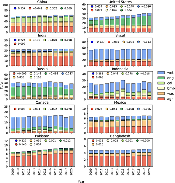
Figure 7. Country-level sectoral emission trends for the period 2009–2020 for large emitting countries. The inset values show the trend (slope) for significant sectors, and the dark blue dot indicates the posterior trend wherever statistically significant (p < 0.1).
Download figure:
Standard image High-resolution imageIn the case of wetland emissions, Russia (0.24 Tg yr–2) and central African countries such as Congo (0.1 Tg yr–2), Democratic Republic of Congo (0.2 Tg yr–2), Sudan (0.02 Tg yr–2), etc. have a positive trend, whereas Bolivia (–0.06 Tg yr–2), Argentina (–0.04 Tg yr–2) and Mexico have a declining trend (figure 6(f)). Central African countries, where wetland emissions constitute a significant source of natural methane emissions, have shown substantial interannual variability since around 2017. These large variabilities were accounted for due to the increased inundation of wetlands (For example, the 2019–2020 surge by (Qu et al 2022).
3.4. Sectoral contributions to country-wise posterior trends
On detailed analysis at the country level, we have calculated the annual total emissions for each sector of the top methane contributors, such as China, the United States, India, Russia, Brazil, Canada, Indonesia, Mexico, Pakistan, and Bangladesh. Trend estimates show whether the posterior emissions in these countries have a significant trend (positive or negative) and which sector is contributing a significant part of the variations. Though we have found some sectors emitting more methane in recent years than at the beginning of the analysis period, some other sectors may have a decreasing trend such that the posterior total emissions may not exhibit any significant trend at all. All the trend values discussed here are Sen's slope estimator significant at a 90% confidence level. Annual sector-wise emissions for the selected countries and the sectors with statistically significant trends in emissions can be found in figure 7.
For the largest emitter of the listed countries, China (∼15% of the global total; UNFCCC) has its posterior emissions growing at 0.56 Tg yr−2 (0.9% of 2009−2020 mean), with contributions from the waste sector growing with 0.35 Tg yr−2 (2.6%) trend with oil and gas following with 0.07 Tg yr−2 (2.8%) with a slight decrease of−0.05 for biomass burning emissions. The positive trend in the oil and gas sector reflects the current policy of transition from coal to gas in China (Qin et al 2017), which has a potential for a growing trend in methane emissions from this sector (e.g. Wang et al 2022), which will continue to increase in the future. The trend of our posterior total in China (0.56 Tg yr−2) is within the range of recently reported trends (0.1–1.7 Tg yr−2, e.g. Zhang et al (2022), table S1) but lower than Zhang et al (2022; 0.73 Tg yr−2), Miller et al (2019; 1.1 Tg yr−2), and greater than Sheng et al (2021; 0.36 Tg yr−2) or Lu et al (2021; 0.25 Tg yr−2). Sheng et al (2021) reported an increasing trend (though weak 0.06 Tg yr−2) for the Chinese waste sector emissions using GOSAT inversion, partially covering our study period. The increasing trend of emission from the waste sector can be attributed to the establishments of more wastewater treatment plants in China. The number of wastewater treatment plants in China has increased by 44% between 2014 to 2019 (Xu et al 2020). Solid waste generation has also been increasing recently (Sheng et al 2021). For the United States, we found a very sharp increase in posterior emissions of around 0.65 Tg yr−2 (1.7%), which is mainly caused by emissions from the oil and gas sector (1.0 Tg yr−2; 7%) and agriculture (0.07 Tg yr−2). At the same time, the coal sector shows a decreasing emission trend of—0.14 Tg yr−2 (–7.3%). Our anthropogenic trend of 1.7% yr−1 is lower than the 2.8 ± 0.3% yr−1 increase reported for 2010–2014 by Turner et al (2016) and higher than the 2006–2015 trend of 0.7 ± 0.3% yr−1 in total U.S. emissions estimated by Lan et al (2019) or 2010–2017 trend of 0.4 Tg yr−2 by Lu et al (2021).
For India, our posterior emission has a trend of 0.22 Tg yr−2, which is 0.75% of the mean. The largest growing sector is the waste sector with 0.12 Tg yr−2 (1.7%), with the oil and gas sector also showing a slight increase of 1.8% per year. The agriculture sector also contributes by a 0.1 Tg yr−2. Brazil's posterior emissions showed no significant trend because the interannual variation is not monotonous. Two sectors showing a substantial increase over the decade are the agriculture and waste sectors, with 0.5 and 2% yr−1 (0.08 and 0.09 Tg), respectively. Pakistan has a trend of 0.22 Tg yr−1 (3%) for posterior emissions, with significant contributions from the agriculture (0.15 Tg), waste, coal, and oil and gas sectors. In Pakistan, almost all sectors show growth between 2 and 3.5%. The fastest-growing cattle populations in the world reported by the United Nations Food and Agriculture Organization (UNFAO) statistics (www.fao.org/faostat, last access: 17 January 2023) over the 2010–2016 period in Pakistan was 1.4 million heads per year. This growing population is reflected in our trend for the agriculture sector.
For Canada, there is a decreasing trend for the coal sector (–2.2%), but with a statistically significant increasing trend in emissions from the oil and gas sector of about 3.2%. Analysis shows a significant decrease in emissions from the oil and gas sector (−2.5%) in Mexico, while the waste sector shows an increasing trend (1.8%). Russia is the second largest producer of oil and gas, but the results indicate a significant decline in associated emissions from this sector (−0.24 Tg yr−2; 2.1%). For Russia, emissions from the agricultural sector show a consistent decreasing trend (−0.01 Tg yr–2) during the period. On the rise is emission from the coal sector, with 4.5% per year (0.11 Tg yr–2)
Another major contributing country to global methane emission is Indonesia, with a mean posterior emission of 27.4 Tg yr–1. Some posterior sectors in Indonesia show a significant positive trend, with the coal sector having 0.27 Tg yr–2 (7.5%), along with the waste and agricultural sector with 0.05 (2.5%) and 0.07 Tg yr–2 (2%) respectively. According to B.P.'s statistical review of the World Energy Report 2021, Indonesia's energy consumption growth rate for coal during 2009−2019 was 9.4%.
3.5. Sensitivity test for the influence of prior emissions on inferred trends
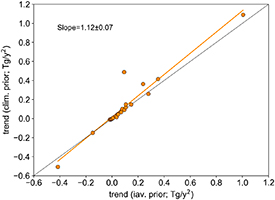
In order to assess whether the inferred emission trends were driven by any interannual variations in the prior fluxes or the observed concentrations, we have conducted inversions based on monthly varying, interannually constant prior fluxes (climatological fields for the 2009–2020 period). The same trend analysis was carried out using the posterior fluxes on country-level aggregated data. The results indicate that the estimated trends in the sensitivity experiment agree well with trends in the posterior using interannually varying priors in most sectors and countries with exceptions of agriculture sector in India (0.092; 0.489), oil and gas sector for the US (1.004;1.09) and Russia (0.237; 0.364), and wetland emission in Russia (−0.416; −0.506) (figure 8). With all these sectors, the emission trend was found to increase in the posterior with climatological prior. Among this, the outlier is the agricultural emissions in India. Some studies (e.g. Ganesan et al 2017) proposed that the emission from ruminants may not be increasing in India and found a non-significant trend for India during 2010–2015, and other studies have reported increasing trends in the areas of rice cultivation (Maasakkers et al 2019). However, as we optimize the agricultural sector together, it is unclear which sector is causing the growth during the study period. Therefore, from the analysis of the sensitivity simulations, it appears that the inferred posterior sectoral trends in our study were not driven by the trends in the prior fluxes.
Figure 8. Comparison of estimated posterior country-level sectoral emission trends (significant at 90%) for interannually varying and climatological prior fluxes. The black line is where the two trends perfectly agree, and the orange line is the regression line between the two sets of trend values.
Download figure:
Standard image High-resolution image
4. Conclusion
We used a high-resolution methane inverse model NTFVAR, a global Eulerian–Lagrangian coupled model that consists of the NIES-TM model as a Eulerian three-dimensional transport model and FLEXPART as the Lagrangian model, to estimate methane emissions using GOSAT data and other ground-based observations for the period 2009–2020. The model optimizes six emission sectors: agriculture, waste, biomass burning, coal, oil and gas, and wetland emission on a biweekly time step on a 0.1° × 0.1° latitude-longitude grid. The estimated emissions for six emission sectors were aggregated to a country level, and the trends were estimated. Our analysis showed that the global total posterior emission has a growth rate of 2.6 Tg yr–2 for the analysis period 2009–2020, with significant contributions from waste (1.01 Tg yr–2) and agriculture (0.9 Tg yr–2) sectors. Most countries had methane emissions from their waste sector growing in the last decade. This can be due to increased consumption depending on the economic development of the region. Specific analyses for each major contributing country to global methane emissions were carried out. Country-level aggregated sectoral emissions showed significant trends in total posterior emissions for China (0.56 Tg yr–2), India (0.22 Tg yr–2), United States (0.65 Tg yr–2), Bangladesh (0.053 Tg yr–2), and Pakistan (0.22 Tg yr–2) among the significant methane emitters. Emission sectors that contribute a substantial part to the trend in these national emissions depend on the country's policies on sources of energy, agricultural production, consumption, etc., which correlates to the growing population. In China, waste (0.35) and oil and gas (0.07 Tg yr–2) contributed to the growth of total methane emissions during the 2009–2020 period. Implementation of policies related to the establishment of wastewater plants to prevent water pollution, as well as the increasing solid waste generation, is the main cause of the growth of emissions from this sector. In the figures for Chinese methane emissions, their policy for the transition from coal to gas is evident from the increasing trend in the oil and gas sector. At the same time, the trend in the coal sector exists without any significant decline (e.g. Miller et al 2019). Indian emissions were significantly driven by the agriculture sector (0.09), waste (0.11 Tg yr–2), and oil and gas sources (1.8%). Our results agree with numerous recent studies on the methane emissions from the oil and gas sector in the United States (1.0 Tg yr–2) with a corresponding reduction in emission from the coal sector (−0.15 Tg yr–). Other countries having statistically significant trends are Brazil (waste 0.09; agriculture 0.08 Tg yr–2), Russia (coal 0.12, wetland 0.24, biomass burning 0.15 and oil and gas −0.42 Tg yr–2), Indonesia (coal 0.28 Tg yr–2), Canada (oil and gas 0.08 Tg yr–2) and Mexico (waste 0.04 Tg yr–2).
In the case of wetland emissions, Russia (0.24 Tg yr–2) and central African countries such as Congo (0.1 Tg yr–2), Zambia (0.02 Tg yr–2), etc. have a positive trend, whereas Bolivia (–0.09 Tg yr–2) and the USA (–0.03 Tg yr–2) have a declining trend. Central African countries, where wetland emissions constitute a significant source of natural methane emissions, have shown a substantial increase since around 2017. Though this exceptional increase reported for recent years was accounted for due to the increased inundation of wetlands (For example, the 2019–2020 surge reported by Qu et al 2022), our trend analysis also shows significant increasing trends for central Africa, northern South America, and Russia. A set of inversions with interannually constant prior fluxes also yielded similar significant trends in major sectors, confirming that the inferred trends are not driven by prior interannual variability. Our study provides a list of countries with significant contributions to the global atmospheric methane growth rate; some of them are known emitters, and some others are emerging as significant contributors due to their economic development. The sectoral as well as posterior total trends discussed in this study show the emission sectors driving the increased emission of these major emitters. We acknowledge that our assumption that the emission sources are not collocated may not hold good over diffuse sources. For example, wetlands and gas leaks may have an impact on the estimated emissions and associated trends for some other sectors, but the assumption is valid for large and intense sources globally. Our study provides a comprehensive accounting of country-level methane emission trends from various source sectors, which is relevant to emission mitigation efforts.
Acknowledgments
We thank the Ministry of the Environment, Japan, for the financial support for the GOSAT project, under which this work was carried out. The simulations were carried out at the supercomputing facility at the National Institute for Environmental Studies, Tsukuba, Japan. The authors acknowledge the PIs and contributors related to the operations in the compilations of the Obspack CH4 dataset (obspack_ch4_1_GLOBALVIEWplus_v4.0_2021-10-14) and ICOS network. The contributions from the following people and institutions are thankfully acknowledged. A di Sarra and S Piacentino (ENEA); A Zahn, F Obersteiner, H Boenisch and T Gehrlein (KIT/IMK); A Desai (UofWI); A Karion (NIST); A Andrews, B Baier, C Sweeney, E Dlugokencky, E Hintsa, F Moore, J B Miller, K McKain and K N Schuldt (NOAA); A Colomb and J M Pichon (OPGC); B Scheeren and H Chen (RUG); B Viner (SRNL); B Stephens (NCAR); C Labuschagne (SAWS); C L Myhre, K Tørseth and O Hermanssen (NILU); C E Miller (NASA-JPL); C-H Lee, H Lee, H -Y Kang and M-Y Ko (KMA); C Plass-Duelmer, D Kubistin, M Schumacher and M Lindauer (DWD); C Gerbig (MPI-BGC); C D Sloop (EN); D Jaffe (UofWA); D Munro (NOAA-CIRES); D Worthy (ECCC); E Kozlova (CEDA); E Gloor (UoL); E Cuevas and P P Rivas (AEMET); E Kort (UoM); G Vitkova, K Kominkova and M V Marek (CAS); G Manca and P Bergamaschi (JRC); G Brailsford and S Nichol (NIWA); H Matsueda (MRI); I Lehner, T Biermann and M Heliasz (LUND-CEC); I Mammarella and P Keronen (UHELS); J W Elkins (HATS); J Müller-Williams (HPB); J Arduini (UNIURB); J Turnbull (GNS); J Lee (UofME); J P DiGangi (NASA-LaRC); J Hatakka, T Laurila and T Aalto (FMI); J Holst and M Mölder (LUND-NATEKO); K Saito (JMA); K Davis, N Miles, S Richardson and T Lauvaux (PSU); L V Gatti (INPE); L Emmenegger and M Steinbacher (EMPA); L Haszpra (RCAES); M K Sha M De Mazière (BIRA-IASB); M Delmotte, M Ramonet, M Lopez and V Kazan (LSCE); M L Fischer and M Torn (LBNL); M Leuenberger (KUP); M Sasakawa, T Machida and Y Niwa (NIES); O Laurent (ICOS-ATC); P Trisolino P Cristofanelli (CNR-ISAC); P Krummel, R Langenfelds and Z Loh (CSIRO); P Shepson (PU); P Smith (SLU); S C Biraud (LBNL-ARM); S Morimoto and S Aoki (TU); S O'Doherty (UNIVBRIS); S Wofsy (HU); S Conil (Andra); T Schuck (IAU); V Ivakhov (MGO).
Data availability statement
The data cannot be made publicly available upon publication due to legal restrictions preventing unrestricted public distribution. The data that support the findings of this study are available upon reasonable request from the authors.
Funding
This research was supported by the GOSAT project (251IAA0) at the National Institute for Environmental Studies, Japan. Measurements at Jungfraujoch were supported by ICOS Switzerland, which is funded by the Swiss National Science Foundation, in-house contributions, and the State Secretariat for Education, Research and Innovation.
Conflict of interest
The authors declare that they have no known competing financial interests or personal relationships that could have appeared to influence the work reported in this paper.
Supplementary data (5.7 MB DOCX)