

Abstract
The sensitivity of urban canopy air temperature ( ) to anthropogenic heat flux (
 ) is known to vary with space and time, but the key factors controlling such spatiotemporal variabilities remain elusive. To quantify the contributions of different physical processes to the magnitude and variability of
  (where
  represents a change), we develop a forcing-feedback framework based on the energy budget of air within the urban canopy layer and apply it to diagnosing
  simulated by the Community Land Model Urban over the contiguous United States (CONUS). In summer, the median
  is around 0.01
  over the CONUS. Besides the direct effect of
  on
on  , there are important feedbacks through changes in the surface temperature, the atmosphere–canopy air heat conductance (
 ), and the surface–canopy air heat conductance. The positive and negative feedbacks nearly cancel each other out and
  is mostly controlled by the direct effect in summer. In winter,
  becomes stronger, with the median value increased by about 20% due to weakened negative feedback associated with
  . The spatial and temporal (both seasonal and diurnal) variability of
  as well as the nonlinear response of
  to
to  are strongly related to the variability of
  , highlighting the importance of correctly parameterizing convective heat transfer in urban canopy models.
Export citation and abstract BibTeX RIS

Original content from this work may be used under the terms of the Creative Commons Attribution 4.0 license. Any further distribution of this work must maintain attribution to the author(s) and the title of the work, journal citation and DOI.
1. Introduction
Anthropogenic heating resulting from energy consumption by human activities is an important controllor of urban climate. Although they occupy only 3% of the Earth's surface, cities consume 60%–80% of global energy and house more than half of the human population (United Nations 2022). The intense anthropogenic heating in cities can increase heat stress (Doan et al 2019, Jin et al 2020, Molnár et al 2020), which threatens thermal comfort and causes heat-related illnesses (Mora et al 2017). Studies have found that air warming of 1 °C is associated with a 1.8% increase in the mortality rate in cities when the daily temperature is higher than 28 °C (Chan et al 2012). Meanwhile, a higher temperature resulting from anthropogenic heating affects cooling energy demand, air quality, ecosystems and so on (Fink et al 2014, Salamanca et al 2014, Xie et al 2016, Liu et al 2020). Anthropogenic heat flux also affects meteorological processes within the urban boundary layer (Fan and Sailor 2005, Chen et al 2009, Suga et al 2009, Krpo et al 2010, Bohnenstengel et al 2014, Zhang et al 2016, Ma et al 2017, Molnár et al 2020, Mei and Yuan 2021).
Anthropogenic heat flux is generated from many sources, including building and industrial energy consumption, traffic and human metabolism (Sailor 2011, Chow et al
2014, Sun et al
2018). The magnitude of anthropogenic heat flux varies strongly with the local climate, population density, economy and technology (Fan and Sailor 2005, Allen et al
2011, Sailor et al
2015, Yang et al
2017, Jin et al
2020). The magnitude of anthropogenic heat flux is also scale dependent. At long-term and city (or larger) scales, the anthropogenic heat flux is typically of the order of 0.1–1  . For example, Sailor et al (2015) developed a national database of anthropogenic heat flux over the contiguous United States (CONUS) and showed that the maximum wintertime (summertime) anthropogenic heat flux is around 0.8–0.97
  (0.47–0.63
  ) across 61 US cities. Another study reported that the annual mean anthropogenic heat flux is around 0.39
  , 0.68
  and 0.22
  for COUNS, western Europe and China, respectively, and only 0.028 W m−2 on the global scale (Flanner 2009). However, the short-term and neighborhood-scale anthropogenic heat flux can be much stronger (Sailor and Lu 2004). Ichinose et al (1999) showed that the anthropogenic heat flux in central Tokyo exceeded 400
  in the daytime, and the maximum value reached 1590
  in the early morning in winter.
Previous studies on the effects of anthropogenic heat flux on urban climate were typically conducted using weather and climate models. Salamanca et al (2014) quantified the impacts of anthropogenic heat flux by turning on/off air conditioning systems in the Weather Research and Forecasting (WRF) model coupled to a building energy model (BEM) and a multilayer building effect parameterization. Their results revealed that the heat emitted from air conditioning systems resulted in a 1 °C–1.5 °C temperature rise during summer nights over Phoenix, USA. Fan and Sailor (2005) incorporated an anthropogenic heating source term in the near-surface energy balance within the NCAR/PennState Fifth Generation Model. They found that the influence of anthropogenic heat flux on the urban climate of Philadelphia, USA was significant, particularly during nighttime and in winter, with near-surface air warming as large as 2 °C–3 °C. Similar results were also found in China (Feng et al 2012, 2014) and Australia (Ma et al 2017), where the temperature rise was more pronounced in winter than summer. In another numerical study conducted in a Japanese megacity (Keihanshin district), the results indicated that although the daytime anthropogenic heat flux was larger than the nighttime counterpart, the induced temperature rise was nearly threefold larger at night (Narumi et al 2009). Studies also revealed that the anthropogenic heating effects depended not only on the quantity of anthropogenic heat flux but also atmospheric stratification and orographic factors (Block et al 2004, Narumi et al 2009, Zhang et al 2016).
Since it is obvious that the amount of warming induced by anthropogenic heating depends on the magnitude of the anthropogenic heat flux, it is perhaps more important to examine the ratio of the temperature increase to the amount of anthropogenic heat flux ( , where
  represents a change), much like the concept of climate sensitivity but at a local (urban) scale. In this sense, we treat the change in anthropogenic heat flux (
 ) as the climate forcing and the change in urban temperature (
 ) as the climate response. Table 1 provides a selected list of existing studies on the warming effect of anthropogenic heat flux. By normalizing the temperature increase by the magnitude of anthropogenic heat flux, a better consistency among different studies emerges, with the magnitude of
  being of the order of 0.01
  . This value is consistent with the findings of Kikegawa et al (2014), who carried out field campaigns based on meteorological measurements and monitoring of electricity demand, as well as numerical simulations with WRF (coupled with a multilayer urban canopy model and a BEM) in two major Japanese cities, Tokyo and Osaka, in July to August 2007. Their work suggested an afternoon sensitivity of
  based on observations and showed that the simulated results had the same order of magnitude. However, it is noteworthy to point out that the magnitude of
  from different studies (table 1) still varies by nearly two orders of magnitude [from 0.001 to 0.05
  ]. More importantly, the physical processes responsible for such variability remain elusive. Quantification of the key factors controlling the variability of
  frames the scope of this study.
Table 1. A selected list of existing studies on the warming effect of anthropogenic heat (AH) emissions. Note that most values for  are rough estimates based on the data in these studies, except for the work of Kikegawa et al (2014).
| Reference | Region | Model | Peak AH ( ) ) | Peak  ( ( ) ) | Estimated  ( ( ) ) |
|---|---|---|---|---|---|
| Ichinose et al (1999) | Tokyo, Japan | The Colorado State University mesoscale model | 1590 | 2.5 | 0.001–0.05 |
| Fan and Sailor (2005) | Philadelphia, USA | NCAR/PennState fifth generation model | 90 | 3 | 0.003–0.03 |
| Narumi et al (2009) | Keihanshin, Japan | Model in Pielke (1974) | 115 | 0.6 | 0.005–0.01 |
| Feng et al (2012) | China | Weather Research and Forecasting (WRF) | 50 | 0.15 | 0.003 |
| de Munck et al (2013) | Paris, France | A coupled model consisting of the non-hydrostatic meso-scale atmospheric model | 34 | 0.5 | 0.015 |
| Bohnenstengel et al (2014) | London, UK | The Met Office-Reading urban surface exchange scheme | 400 | 3 | 0.008 |
| Kikegawa et al (2014) | Tokyo and Osaka, Japan | Observations and WRF–canopy model–building energy model | 220 | — | 0.005–0.012 |
| Feng et al (2014) | East China | WRF | 45 | 0.9 | 0.02 |
| Wang et al (2015) | Yangtze River Delta | WRF | 50 | 0.9 | 0.018 |
| Zhang et al (2016) | Pearl River Delta, China | WRF | 405 | 3.37 | 0.008 |
| Ma et al (2017) | Sydney, Australia | WRF | 60 | 1.5 | 0.025 |
| Doan et al (2019) | Hanoi, Vietnam | WRF | 100 | 0.7 | 0.007 |
| Yang et al (2019) | Yangtze River Delta, China | WRF | 150 | 1 | 0.007 |
| Molnár et al (2020) | Szeged, Hungary | WRF | 31 | 1.5 | 0.05 |
| Mei and Yuan (2021) | Newton, Singapore | An analytical model and large eddy simulation | 15 | 0.45 | 0.03 |
To achieve this, we develop a forcing-feedback framework based on the energy budget of air within the urban canopy layer (UCL, i.e. the layer below the height of the main urban elements) and apply it to diagnosing  simulated by the Community Land Model Urban (CLMU) over the CONUS. This region, characterized by a growing urban population and significant energy consumption, has not yet been thoroughly investigated in terms of the impact of anthropogenic heat flux. This study is organized as follows: section 2 describes the forcing-feedback framework and model experiments. Section 3 evaluates
  at the seasonal and diurnal scales. The key feedback mechanisms and the factors controlling the variability of
  are discussed in detail in this section. Finally, discussions and conclusions are presented in sections 4 and 5, respectively.
2. Methodology
2.1. A forcing-feedback framework
We propose a forcing-feedback framework to diagnose the sensitivity of air temperature within the UCL, also called urban canopy air temperature hereafter, to anthropogenic heat flux based on the energy budget of air within the UCL (figure 1). This conceptualization of the UCL is consistent with the theoretical underpinning of nearly all single-layer urban canopy models (UCMs) in weather and climate modeling, including the CLMU to be used in this study (more details on the CLMU are presented later). Our starting point is that the UCL is our control volume (or system of interest) and is the direct recipient of anthropogenic heat flux (i.e. the forcing). At steady state, the energy budget of the air within the UCL can be written as

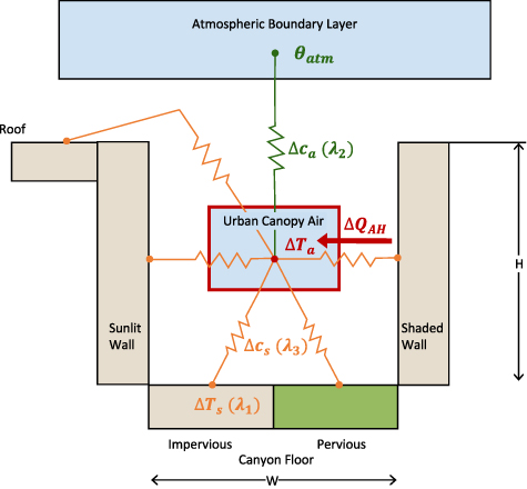
Figure 1. Schematic of the forcing-feedback framework for understanding the impact of anthropogenic heat flux ( ) on urban canopy air temperature (
 ). In this framework, the anthropogenic heat flux perturbs the energy budget of the air within the UCL, directly altering
  and further influencing the changes in surface temperatures (
 ) of multiple urban facets, the heat conductance between the canopy air and urban surfaces (
 ) and the heat conductance between the canopy air and overlying atmosphere (
 ). Besides the direct effect of
  on
on  , there also exist important feedbacks:
  refers to the strength of feedback from
  ;
;  is the feedback parameter for
  ;
;  is the feedback parameter for
  . Source: adapted from Oleson et al (2010) © 2010 UCAR.
Download figure:
Standard image High-resolution imagewhere  is the anthropogenic heat flux and
  is the sum of heat fluxes other than the anthropogenic heat flux (we shall say more about
  later). When the anthropogenic heat flux is altered by a certain amount (indicated by
  ), the energy balance of air within the UCL reaches a new equilibrium state

where  can be interpreted as the added anthropogenic heat flux compared with the scenario without anthropogenic heat flux and
  is the total change of other heat fluxes in response to
  .
.
Changes in other heat fluxes ( ) are often related to changes in the urban canopy air temperature (
 ). Denoting
  , we can write the sensitivity of urban canopy air temperature to anthropogenic heat flux as
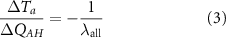
where  is the sensitivity parameter (called the total sensitivity parameter in order to distinguish it from other feedback parameters introduced later). The sensitivity
  , which indicates how easily the urban canopy air temperature can be altered by a perturbation of anthropogenic heat flux, is thus equivalent to the negative reciprocal of the total sensitivity parameter (
 ). If the absolute value of
  is larger, the urban canopy air warming per unit increase of anthropogenic heat flux is weaker. Therefore, to understand
  , we need to examine
  in the relation
  .
.
The air within the UCL receives convective heat fluxes from various urban surfaces and the overlying atmosphere. The sum of these heat fluxes ( ) received by the air within the UCL can thus be written as
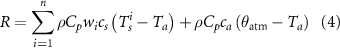
where  is the number of urban surfaces (e.g. there are five urban surfaces in the CLMU that interact with the urban canopy air, including roof, previous ground, imperious ground, sun wall and shade wall),
  refers to the
  urban surface,
  is the weight of the
  surface based on the corresponding area fraction (converted to per unit area of urban canyon floor in the horizontal direction),
  is the air density (kg m−3),
  is the specific heat of air at constant pressure, assumed to be of a constant value of 1004.64 J kg−1 K−1,
  is the heat conductance between the air within the UCL and the urban surface (called the surface–canopy air heat conductance, m s−1),
  is the heat conductance between the air within the UCL and the overlying atmosphere (called the atmosphere–canopy air heat conductance, m s−1),
  is the urban surface temperature (K) and
  is the atmospheric potential temperature (K). Here we have assumed that the heat conductances between the air within the UCL and different urban surfaces are identical, which is a common assumption made in the CLMU and many other single-layer UCMs. But this assumption can be relaxed by allowing
  to vary for different urban surfaces in future work.
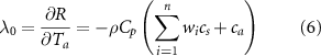
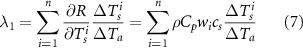
With equation (4),  can be written as the sum of the direct effect and feedbacks. Using the chain rule on equation (4) yields

where the partial and total derivatives are denoted by  and
and  , respectively. In this equation,
  is the baseline sensitivity parameter, representing the direct effect of anthropogenic heat flux on urban canopy air temperature, with everything else (e.g. surface temperature, atmosphere–canopy air heat conductance, etc) held the same. Other
  parameters represent different feedback processes:
  refers to the strength of feedback from changes in surface temperatures;
  is the feedback parameter for changes in atmosphere–canopy air heat conductance;
  is the feedback parameter for changes in surface–canopy air heat conductance;
  is the parameter for atmospheric feedback. A positive (or negative) feedback means that the process leads to an amplification (or dampening) of the direct effect of anthropogenic heat flux on urban canopy air temperature.
Combining equations (4) and (5), the baseline sensitivity parameter and feedback parameters can be derived as
Equations (1)–(10) constitute our forcing-feedback framework for diagnosing the sensitivity of urban canopy air temperature to anthropogenic heat flux. The aim of the proposed forcing-feedback framework is not to predict  but to provide a diagnostic tool for quantifying the strengths of direct effects and feedback processes. In this study, the inputs for this framework are the simulated results from the CLMU. However, this framework is not limited to the CLMU and can be applied to diagnosing outputs from other UCMs.
2.2. The CLMU model and the numerical experiment design
The CLMU model represents urban parameterization within the Community Land Model (CLM), which is the land component of the Community Earth System Model (CESM) (Danabasoglu et al 2020). In this study, the most recent released version of the CLM (CLM5) within the framework of CESM version 2 (CESM2) is used. Within each land grid cell, CLM5 can have multiple land units including vegetated, crop, urban, glacier and lakes. For each urban land unit, three urban categories (tall building district, high density and medium density) are allowed. In CLMU, the urban canyon system consists of five surfaces: roofs, sunlit and shaded walls, impervious and pervious floors. The energy and water fluxes from each urban surface interact with the canopy air (see figure 1). A more detailed description of CLMU including the main urban parameters can be found elsewhere (Oleson et al 2010, Oleson and Feddema 2020). The CLMU input data are supplied by a global dataset (Jackson et al 2010). The model has been widely used to study urban energy and water fluxes, as well as surface and air temperatures (Oleson et al 2008a, 2008b, Grimmond et al 2011, Demuzere et al 2013, Karsisto et al 2016, Oleson and Feddema 2020). In this study, we use an improved CLMU that includes parameterizations of urban heat mitigation strategies (e.g. cool roofs and green roofs) that have been proposed and validated in our previous work (Wang et al 2020, 2021), although these new features are not used in this study.
We run CLM5 in an offline mode (i.e. forced by meteorological data) at a 1/8 degree spatial resolution over the CONUS and at an hourly time step (Wang and Li 2022). The hourly meteorological forcing data are from the North America Land Data Assimilation System phase II (NLDAS2) dataset (Xia et al
2012). The model is first spun up for 84 years by recycling the 1979–1999 NLDAS2 forcing four times. Four sets of numerical experiments are then conducted from 1979 to 1999 using the same initial condition obtained from the spin-up run (table S1). These four numerical experiments are designed to quantify how the urban canopy air temperature (figure 1) responds to a prescribed increase anthropogenic heat flux. In the control (CTL) experiment, no anthropogenic heat flux is added to the urban canopy air heat budget, and the simulated canopy air temperature is denoted as  . In the first sensitivity experiment (AH1), we add 1
  of anthropogenic heat flux into the urban canopy air heat budget at each time step and compute a new canopy air temperature (hereafter
  ). Therefore, the difference between
  and
and  (which is numerically equivalent to
  given that the added anthropogenic heat flux is 1
  ) is the total impact of 1
  of anthropogenic heat flux, which includes both the direct effect and the feedbacks. In another two sensitivity experiments AH10 and AH100, the added anthropogenic heat flux is 10
  and 100
  , respectively. We denote the simulated urban canopy air temperatures in these two experiments as
  and
and  , respectively. The sensitivity
  is thus calculated as
  and
and  , respectively (see table S1). These two sensitivity experiments (AH10 and AH100) are designed to quantify whether the sensitivity
  is influenced by the magnitude of anthropogenic heat flux due to nonlinearity in the feedback processes. We choose these values (1, 10, 100
  ) to cover a wide but reasonable range of anthropogenic heat fluxes.
We should emphasize that the added anthropogenic heat flux in all our experiments is prescribed, not computed by the BEM in CLMU (Oleson et al
2011, Demuzere et al
2013). We prescribe the added anthropogenic heat flux because we are mostly interested in the sensitivity of urban canopy air temperature to anthropogenic heat flux, not what processes generate the anthropogenic heat flux. Moreover, when the BEM in CLMU is used, the generated anthropogenic heat flux is added to the pervious and impervious surface energy budgets, which seems unphysical and is avoided in our study. Another way of interpreting our results is that they represent the sensitivity of urban canopy air temperature to anthropogenic heat fluxes from non-building (e.g. transportation) sectors with magnitudes of 1, 10 and 100  .
.
For all simulations, we output the hourly urban canopy air temperature, the temperatures of different urban surfaces (i.e. roofs, walls and canyon floors), the atmospheric potential temperature, the surface–canopy air heat conductance ( ), as well as the atmosphere–canopy air heat conductance (
 ). Note that the outputted
  and
and  are computed internally via their parameterizations in CLMU. These hourly outputs are then used in the forcing-feedback framework described in section 2.1. Specifically, we compute the hourly sensitivity parameters based on equations (6)–(9). Given that we do not have atmospheric feedbacks in our simulations,
  . With the sensitivity parameters calculated using equations (6)–(9), the total sensitivity
  can be diagnosed using equations (3) and (5). The diagnosed
  is then compared with the directly computed
  mentioned above (e.g. for AH1 the directly computed
  is simply
  ). We average the hourly results over 20 years from 1980 to 1999.
Before we move to the results section, it is informative to briefly discuss the physics behind  and
and  and their parameterizations in CLMU, as they are key parameters in the forcing-feedback framework (see, e.g., equation (6)). Physically,
  (
( ) represents the efficiency of convective heat transfer between the overlying atmosphere (the urban surfaces) and the canopy air. Given that the flow within the UCL is turbulent, both
  and
and  are strongly affected by shear and buoyancy, the two main sources of turbulence kinetic energy. However,
  and
and  are fundamentally different because they represent the convective heat transfer efficiencies across different levels. In terms of their parameterizations in CLMU,
  is parameterized through the classic Monin–Obukhov similarity theory (Oleson et al
2008a). Hence,
is parameterized through the classic Monin–Obukhov similarity theory (Oleson et al
2008a). Hence,  is strongly affected by atmospheric stratification. However,
  is parameterized as a function of wind speed alone in the urban canyon (Oleson et al
2008a) and is thus much less affected by atmospheric stratification than
is parameterized as a function of wind speed alone in the urban canyon (Oleson et al
2008a) and is thus much less affected by atmospheric stratification than  .
.
3. Results
3.1. Sensitivity of urban canopy air temperature to anthropogenic heat flux ( ) and the associated feedback parameters

We first present the sensitivity  simulated by CLMU in summer (June–August, or JJA) and winter (December–February, or DJF) seasons (figure 2). The results shown here have been averaged over 20 years (1980–1999) and are based on the AH1 experiment where the added anthropogenic heat flux is 1
  . The effect of increasing the magnitude of anthropogenic heat flux will be discussed in section 3.4. In summer, the median value of
  is around 0.01
  , broadly comparable with previous studies presented in table 1. Here the median values are shown to minimize the influence of outliers. In winter,
  becomes stronger, with the median value increased by about 20%. In some cities in the southwestern USA (e.g. Los Angeles and Phoenix), the winter values of
  even reach 0.03
  .
.

Figure 2. The sensitivity of urban canopy air temperature to anthropogenic heat flux  simulated by CLMU and diagnosed from the proposed forcing-feedback framework. Parts (a), (c), (e) are for JJA, (b), (d), (f) are for DJF and (e), (f) are histograms for
  . The median value over the CONUS is also shown at the top right of each map. All units are
  . The results are from AH1. Only grid cells with more than 0.1% of urban land are shown and analyzed.
Download figure:
Standard image High-resolution imageTo understand the directly computed  from CLMU simulation results, we employ the forcing-feedback framework described in section 2.1. The total sensitivity diagnosed from this framework (i.e. using equations (5)–(9)) matches very well with the directly computed
  (figure 2), with spatial correlation coefficients larger than 0.99. These results give us confidence to use the forcing-feedback framework to interpret
  .
.
Based on the forcing-feedback framework, the total sensitivity parameter ( ) can be decomposed into the sum of the baseline sensitivity parameter (
 ) and the feedback parameters (
 and
and  ). We find that the magnitude of
  is almost identical to the magnitude of
  (the spatial median value is −122
  for both
  and
and  in summer (figure 3). This is because the sum of the three feedback parameters (
 ) is very small, with the positive feedbacks and negative feedbacks nearly canceling each other. The positive feedback is mainly from changes in surface temperature (
 , with a median value of 24
 ). This is expected as increases in surface temperature due to the added anthropogenic heat flux can in turn amplify the urban canopy air warming. On the other hand, the negative feedback is mainly the result of changes in atmosphere–canopy air heat conductance (
 , with a median value of −25
 ). As the anthropogenic heat flux is added, the atmospheric stratification is altered (i.e. relatively more unstable), resulting in increased atmosphere–canopy air heat conductance (
 ). This in turn leads to an increase in heat transfer into the overlying atmosphere and a dampening of the urban canopy air warming signal. The feedback from changes in surface–canopy air heat conductance (
 , with a median value of 1
 ) is much weaker than the other two feedback processes. This can be explained by the parameterization of surface–canopy air heat conductance (
 ) in CLMU, which is only dependent on the wind speed in the UCL and is thus a much weaker function of atmospheric stratification than the atmosphere–canopy air heat conductance (
 ).
).

Figure 3. The sensitivity and feedback parameters: (a), (b) the total sensitivity parameter ( ); (c), (d) the baseline sensitivity parameter (
 ); (e)–(g) the feedback parameter for surface temperature (
 ) ((e), (f)), heat conductance between the canopy air and overlying atmosphere (
 ) ((g), (h)), and heat conductance between the canopy air and urban surfaces (
 ) ((i), (j)). Parts (a), (c), (e), (g) and (i) are for JJA and (b), (d), (f), (h) and (j) are for DJF. The median value over the CONUS is also shown at the top right of each map. All units are
  . The results are from AH1. Only grid cells with more than 0.1% urban land are shown.
Download figure:
Standard image High-resolution imageIn winter (figure 3), the negative feedback from atmosphere–canopy air heat conductance ( ) decreases in magnitude by 11
 (in terms of median value) when compared with its summer counterpart (see also figure S1 for a comparison between summer and winter results). Namely,
  becomes less negative, implying that the negative feedback from atmosphere–canopy air heat conductance (
 ) is weakened. Unlike the reduced magnitude of
  in winter, the winter–summer differences in
  and
and  are much smaller (about 1
 in terms of median values) and almost negligible. As a result, the sum of feedbacks (
 ) becomes positive in winter (compared with nearly zero in summer). The absolute value of the total sensitivity parameter (
 ) therefore decreases, which further leads to an increase in
  . The weakened negative feedback from atmosphere–canopy air heat conductance (
 ) explains why stronger canopy air warming is observed in winter than in summer with the same amount of anthropogenic heat flux (figure 2), a typical result in the literature.
3.2. Spatial variability of and its controlling factors

Figure 2 shows the strong spatial variabilities in  . To understand these spatial variabilities, we first note that the spatial pattern of the baseline sensitivity parameter
  is very close to that of
  , with spatial correlation coefficients of 0.77 and 0.95 in summer and winter, respectively. Therefore, the spatial variability of
  largely determines the spatial variability of
  . From equation (6),
  is proportional to the sum of atmosphere–canopy air heat conductance (
 ) and surface–canopy air heat conductance (
 ). We find that
  is less than 20% of
  and shows little spatial variability (not shown). As a result, one would expect that the spatial variability of
  is mainly controlled by the spatial variability of
  .
.
This is indeed the case. We find that the spatial correlation coefficients between  and
and  are very strong (−0.87 and −0.98 in summer and winter, respectively). The negative correlations are understandable since physically the atmosphere–canopy air heat conductance (
 ) indicates how strongly the air within the UCL communicates with the overlying atmosphere in terms of convective heat transfer. In places with larger (smaller)
  , it is easier (more difficult) to transfer heat from the UCL to the overlying atmosphere, and thus the canopy air warming signal is weaker (stronger) with the same amount of anthropogenic heat flux.
3.3. Diurnal variation of and its controlling factors

We further analyze the diurnal variation of  . To do this, we select four metropolitan cities that have widely different climates and geographical locations (San Francisco, Boston, Chicago and Houston), instead of presenting averaged results over the CONUS.
In summer (figure 4(a)), all four cities experience a higher  in the early morning than at other times. The morning peak of
  is around 0.038
  in Houston, followed by San Francisco, Boston and Chicago. In the afternoon, the sensitivity in all cities is close to 0.01
  , which is consistent with the findings of Kikegawa et al (2014) that also suggested a summer afternoon sensitivity of 0.01
  . In contrast, there exist large differences in the diurnal variation of
  in winter (figure 4(b)). The sensitivity
  in Boston and Chicago is around 0.01
  throughout the day with small diurnal variations, while the diurnal variations of
  in Houston and San Francisco are strong, with much larger nighttime values than daytime values. San Francisco has the largest sensitivity in winter among the four cities, with a peak value of 0.036
  .
.

Figure 4. Diurnal cycles of (a), (b) the sensitivity  [unit
[unit  ] and feedback parameters
  ((c), (d)),
  ((e), (f)),
  ((g), (h)),
  ((i), (j)) and
  ((k), (l)) (all in units of
  ) in four cities (San Francisco, Boston, Chicago and Houston). Parts (a), (c), (e), (g), (i) and (k) are for JJA and (b), (d), (f), (h), (j) and (l) are for DJF.
Download figure:
Standard image High-resolution imageAccording to the forcing-feedback framework, the diurnal variations of  are linked to the diurnal variations of feedback parameters, including the baseline sensitivity parameter (
 ). As shown in figures 4(c)–(l),
  and, to a lesser extent,
  exhibit diurnal variations that resemble those of
  , implying that the diurnal variations of
  are controlled by processes encoded in
  (equation (6)) and, to a lesser extent,
  (equation (8)). Close inspection of equations (6) and (8) indicates that a common process in equations (6) and (8) is the atmosphere–canopy air heat conductance (
 ), suggesting that the diurnal variation of
  (and
(and  ) are the key to understanding the diurnal variation of
  .
.
The  is controlled by shear- and buoyancy-generated turbulence and thus is strongly affected by atmospheric stratification. In winter, the air within the UCL experiences more stable conditions at night, and hence
  is smaller,
  is less negative (figure 4(f)) and
  is larger (figure 4(b)) than their daytime counterparts, assuming that the shear is the same between daytime and nighttime. In summer, the accumulation of stable stratification throughout the night reduces
  (leading to a less negative
  , figure 4(e)) and increases
  (figure 4(a)). After sunrise, the stratification transitions from stable to unstable, which increases
  , causes a more negative
  and reduces
  . These two processes yield a morning peak of
  , as observed in figure 4(a). Shear also plays an important role. For example, the stronger winds in Boston and Chicago in winter are likely to cause larger shear, leading to a larger
  and smaller
  , when compared with Houston and San Francisco (figure 4(b)).
3.4. Nonlinear response of to


The above results are from the AH1 experiment, which adds 1  of anthropogenic heat flux into the UCL. We also conduct experiments to investigate how the urban canopy air temperature responds to different amounts of anthropogenic heat flux. The aim of these experiments is to test whether any of the feedbacks scale nonlinearly with
  , thereby creating nonlinear responses of
  to
to  . Note that the baseline sensitivity parameter (
 , see equation (6)) does not change with the magnitude of anthropogenic heat flux. Thus, any nonlinear response must stem from the feedback processes.
Figure 5 presents the relative changes in  and feedback parameters (
 ,
,  ,
,  ) by comparing AH10 and AH100 with AH1 (i.e. the results of AH10 and AH100 minus the results of AH1 and then normalized by the results of AH1). The relative changes in
  are all negative, implying that the sensitivity becomes smaller as the magnitude of anthropogenic heat flux increases. The relative changes between AH100 and AH1 in terms of
  have median values of −27% and −35% in summer and winter, respectively. This suggests that
  does respond nonlinearly to
  . Here we should stress that this result does not mean that changes in urban canopy air temperature
  become smaller as the magnitude of anthropogenic heat flux increases. It is rather
  that reduces as the magnitude of the anthropogenic heat flux increases.

Figure 5. Relative changes (represented by  , %) in (a), (b) the sensitivity
  and feedback parameters
  ((c), (d)),
  ((e), (f)) and
  ((g), (h)) by comparing AH10 and AH100 to AH1 (i.e. the results of AH10 and AH100 minus the results of AH1 and then normalized by the results of AH1). The error bars show 95% confidence interval over the CONUS. Parts (a), (c), (e) and (g) are for JJA and (b), (d), (f) and (h) are for DJF.
Download figure:
Standard image High-resolution image
The relative changes in feedback parameters suggest that the nonlinear response of urban canopy air warming to the addition of anthropogenic heat flux is mostly due to decreases in  (i.e.
(i.e.  becomes more negative) as
  increases (figure 5). For example, the differences between AH100 and AH1 in terms of
  give median values of −13% and −28% in summer and winter, respectively. As alluded to earlier in section 3.1,
  is associated with changes in the atmosphere–canopy air heat conductance (
 ). These results imply that with a larger
  , the increase in
  is stronger, leading to a more negative
  and a weaker
  . Therefore, the nonlinear response of
  to
to  is traced to the role of
4. Discussion
This study has several implications that are important to appreciate. First, we emphasize that it is equally important to study the sensitivity ( ) in addition to the forcing magnitude (
 ). The sensitivity is the ratio of the response (
 ) to the forcing and is a much better constrained quantity than the response itself, as can be seen from table 1. Second, the forcing-feedback framework further allows us to understand why many previous studies reported a
  value of approximately 0.01
  . Without considering any feedbacks and any role for
  (both are reasonably good assumptions), the baseline sensitivity is
  W m−2 K−1 (
 kg m−3,
  J kg−1 K−1 and
  m s−1), yielding a
  of 0.01
  . Third, the forcing-feedback framework allows us to quantify the contributions of various physical processes to the spatiotemporal variability of
  . Our results demonstrate that the atmosphere–canopy air heat conductance (
 ) plays a key role in controlling the spatiotemporal variations of
  , as well as the nonlinear response of
  to
to  . Hence, it is critical for UCMs to accurately represent the convective heat transfer between the canopy air and the overlying atmosphere, among other things. Currently, Monin–Obukhov similarity theory remains the workhorse model for parameterizing
  in UCMs due to its popularity and parsimony (e.g. in the CLMU, see Oleson et al
2008a), even though urban areas are not homogeneous and thus Monin–Obukhov similarity theory does not strictly apply (Garratt 1994). It remains unclear whether Monin–Obukhov similarity theory combined with urban roughness lengths is sufficient for parameterizing
in UCMs due to its popularity and parsimony (e.g. in the CLMU, see Oleson et al
2008a), even though urban areas are not homogeneous and thus Monin–Obukhov similarity theory does not strictly apply (Garratt 1994). It remains unclear whether Monin–Obukhov similarity theory combined with urban roughness lengths is sufficient for parameterizing  over urban areas or if new theories accounting for the effects of urban canopies (e.g. similar to the work by Harman and Finnigan (2007, 2008), see also Bonan et al (2018)) are needed. Furthermore, in this context nearly all UCMs assume that turbulent transport is the only process that needs to be parameterized. However, dispersive transport might become relevant over areas with large variations of building heights (Akinlabi et al
2022). Addressing these questions is outside the scope of this study but is strongly needed.
over urban areas or if new theories accounting for the effects of urban canopies (e.g. similar to the work by Harman and Finnigan (2007, 2008), see also Bonan et al (2018)) are needed. Furthermore, in this context nearly all UCMs assume that turbulent transport is the only process that needs to be parameterized. However, dispersive transport might become relevant over areas with large variations of building heights (Akinlabi et al
2022). Addressing these questions is outside the scope of this study but is strongly needed.
There are also limitations of this work that need to be pointed out. First, we only evaluate the feedback processes within the UCL. Quantifying the role of atmospheric feedback ( ) and how it is scale-dependent (Li and Wang 2019) is left for future work. Second, while we highlight the key role played by the atmosphere–canopy air heat conductance (
 ), diagnosing the physical processes as well as urban morphological parameters that give rise to the spatiotemporal variability of
  (e.g. diagnosing the differences between different cities in figure 4) remains to be conducted. Within the confines of Monin–Obukhov similarity theory,
  is affected by shear-generated and buoyancy-generated turbulence and is a function of mean wind speed, roughness lengths (both momentum and thermal roughness lengths) and stability parameters. The momentum roughness length is further a complex function of building height and canyon geometry. Understanding the spatiotemporal variability of
  and its relation to these underlying factors is beyond the scope of this study. Third, this study does not prescribe spatially and temporally varying anthropogenic heat flux. This is justified by the focus of this work on the sensitivity (
 ) instead of the response (
 ).
).  can be viewed as the product of
  and the forcing
 . Thus, the spatiotemporal variability of the temperature response is further complicated by the spatiotemporal variability of the forcing. Studies aiming to quantify the temperature response should also address the variability of the forcing.
5. Conclusion
Anthropogenic heat flux is an important controlling factor of the urban thermal environment. Although many studies have investigated the impacts of anthropogenic heat flux, the key factors controlling the magnitude of the sensitivity of urban air temperature to anthropogenic heat flux ( ) and its spatial and temporal patterns remain elusive. In this study, we develop a forcing-feedback framework based on the energy balance of air within the UCL and apply the framework to diagnosing simulated
  over the CONUS by a numerical model. Within the forcing-feedback framework,
  is decomposed into the direct effect of
  on
on  , as well as feedbacks through changes in the surface temperature (
 ), the atmosphere–canopy air heat conductance (
 ), and the surface–canopy air heat conductance (
 ). This forcing-feedback framework allows us, for the first time, to understand the contributions of physical processes within the UCL to
  and the spatiotemporal variability of
  in a quantitative manner.
Our study first examines the seasonal variation of  . In summer, the positive feedback (mainly from changes in surface temperature, represented by
  ) is nearly canceled by the negative feedback (mainly from changes in atmosphere–canopy air heat conductance
  , represented by
  ). As a result,
  is dominated by the direct effect (represented by
  ). In winter, the negative feedback from
  (represented by
  ) weakens, leading to a stronger
  . We also investigate the diurnal variations of
  . The results show that the diurnal variations of
  are mostly controlled by the diurnal variations in
  , and to a lesser extent,
  , both of which are strongly related to the diurnal variations of
  (and
(and  ). Hence, it can be summarized that the temporal (both seasonal and diurnal) dynamics of
  are mostly controlled by those of
  . We also find that the spatial variability of
  over the CONUS is mainly determined by the direct effect (
 ). Since
  is proportional to the sum of
  and
and  , and
, and  shows little spatial variability, the spatial variability of
  is dominated by the spatial variability of
  . We further examine the nonlinearity in the response of
  to
to  by varying the magnitude of
  . The nonlinear response of
  to
to  stems mostly from the feedback process associated with changes in atmosphere–canopy air heat conductance (
 ). Our framework provides a tool for studying the feedback mechanisms that are important for understanding the sensitivity of urban canopy air temperature to anthropogenic heat flux.
Acknowledgments
L W and D L acknowledge the financial support by the US Department of Energy, Office of Science, as part of research in Multi-Sector Dynamics, Earth and Environmental System Modelling Program. The computing and data storage resources were provided by the National Energy Research Scientific Computing Center (NERSC), which is supported by the Office of Science of the US Department under contract no DE-AC02-05Ch11231. D L also acknowledges support from the US National Science Foundation (Grant ICER-1854706). T S is supported by UKRI NERC Independent Research Fellowship (NE/P018637/2). W Z is supported by the US DOE Office of Science Biological and Environmental Research as part of the Regional and Global Modeling and Analysis program. The authors are grateful to Dr Keith Oleson at NCAR for insightful discussions.
Data availability statement
The CESM2 release code (release-cesm2.0.1) and input data are available at https://escomp.github.io/CESM/versions/cesm2.1/html/downloading_cesm.html. The data that support the findings of this study are openly available at the following URL/DOI: https://doi.org/10.57931/1890465.
Supplementary data (0.1 MB PDF)